Galaxy and Mass Assembly (GAMA) : Impact of the Group Environment on Galaxy Star Formation

arXiv:1803.05076v1 [astro-ph.GA] 13 Mar 2018

GALAXY AND MASS ASSEMBLY (GAMA): IMPACT OF THE GROUP ENVIRONMENT ON GALAXY STAR FORMATION

S. Barsanti,1 M. S. Owers,1, 2 S. Brough,3 L. J. M. Davies,4 S. P. Driver,4, 5 M. L. P. Gunawardhana,6 B. W. Holwerda,7 _{J. Liske,}8 _{J. Loveday,}9 _{K. A. Pimbblet,}10, 11 _{A. S. G. Robotham,}4 _{and E. N. Taylor}12

1_{Department of Physics and Astronomy, Macquarie University, NSW 2109, Australia} 2_{The Australian Astronomical Observatory, 105 Delhi Rd, North Ryde, NSW 2113, Australia} 3_{School of Physics, University of New South Wales, NSW 2052, Australia}

4_{International Centre for Radio Astronomy Research (ICRAR), University of Western Australia, 35 Stirling Highway, Crawley, WA 6009,}

Australia

5_{School of Physics and Astronomy, University of St Andrews, North Haugh, St Andrews KY16 9SS, UK}

6_{Institute for Computational Cosmology, Department of Physics, Durham University, South Road, Durham DH1 3LE, UK} 7_{University of Leiden, Sterrenwacht Leiden Niels Bohrweg 2, NL-2333 CA Leiden, The Netherlands}

8_{Hamburger Sternwarte, Universit¨at Hamburg, Gojenbergsweg 112,D-21029 Hamburg, Germany} 9_{Astronomy Centre, University of Sussex, Falmer, Brighton BN1 9QH, UK}

10_{E. A. Milne Centre for Astrophysics, University of Hull, Cottingham Road, Kingston Upon Hull HU6 7RX, UK} 11_{School of Physics and Astronomy, Monash University, Clayton, VIC 3800, Australia}

12_{Centre for Astrophysics and Supercomputing, Swinburne University of Technology, Hawthorn 3122, Australia}

(Received November 6, 2017; Revised March 5, 2018; Accepted March 9, 2018)

Submitted to ApJ

Abstract

We explore how the group environment may affect the evolution of star-forming galaxies. We select 1197 Galaxy And Mass Assembly (GAMA) groups at 0.05≤z≤0.2 and analyze the projected phase space (PPS) diagram, i.e. the galaxy velocity as a function of projected group-centric radius, as a local environmental metric in the low-mass halo regime 1012_≤(M

200/M⊙)<1014. We study the properties of star-forming group galaxies, exploring the correlation

of star formation rate (SFR) with radial distance and stellar mass. We find that the fraction of star-forming group members is higher in the PPS regions dominated by recently accreted galaxies, whereas passive galaxies dominate the virialized regions. We observe a small decline in specific SFR of star-forming galaxies towards the group center by a factor∼1.2 with respect to field galaxies. Similar to cluster studies, we conclude for low-mass halos that star-forming group galaxies represent an infalling population from the field to the halo and show suppressed star formation.

Keywords: galaxies: evolution – galaxies: groups: general – galaxies: kinematics and dynamics –

galaxies: star formation

1. INTRODUCTION

The properties of galaxies, such as their star forma-tion rate (SFR), morphology and stellar mass, corre-late strongly with the galaxy number density in the surrounding Universe (Dressler 1980; Kodama & Smail 2001; Smith et al. 2005; Peng et al. 2010). This corre-lation is most visible in galaxy clusters, which are the largest halos that have had time to virialize in the Uni-verse, where their cores are found to be dominated by passive galaxies while in their outskirts there is a higher fraction of star-forming galaxies (e.g., Balogh et al. 1997; Hashimoto et al. 1998; Poggianti et al. 1999;

Couch et al. 2001). The observed correlation with cluster-centric radius reveals radial distance as a crude metric of the time since a particular galaxy has entered the cluster environment - with core galaxies being early virialized cluster members and populations at large radii being increasingly dominated by recently infalling galaxies. However, equating radial distance to the time since infall is a blunt approach as this does not take into account projection effects, and washes out poten-tially important populations such as, first-pass infalling galaxies which happen to be in the cluster core at the time of observation, backsplash galaxies which have al-ready traversed the cluster core and are observed close to the maximum distance before their second infall, and galaxies which have already undergone multiple passes but appear at large radii. A more sophisticated ap-proach is to classify galaxies based on both position and velocity, considering their dynamical state within the cluster. The projected phase space diagram (PPS), i.e. the galaxy velocity as a function of projected cluster-centric radius, has been extensively used to separate the different cluster populations and to study their spec-tral features (e.g.,Pimbblet et al. 2006; Mahajan et al. 2011; Oman et al. 2013; Muzzin et al. 2014; Jaff´e et al. 2015; Oman & Hudson 2016). These works show that galaxy spectral properties correlate strongly with their position on the PPS. Finally, there is evidence for a rela-tionship between SFR and galaxy density and projected cluster-centric radius, in the sense that star-forming galaxies in clusters show suppressed star formation with respect to field galaxies, and many studies have been dedicated to understanding the underlying physics driv-ing this suppression in galaxy clusters (e.g.,Lewis et al. 2002; G´omez et al. 2003; von der Linden et al. 2010;

Paccagnella et al. 2016).

The PPS and the role of the environmental mecha-nisms in affecting galaxy star formation are less clear in low-mass halos, i.e. galaxy groups with mass ∼ 1012−1014M⊙. Galaxy groups are the most common

galaxy environment (Eke et al. 2005) and their study

offers an important tool for a more complete under-standing of galaxy formation and evolution. Similar to cluster environments, several works have found that the galaxy morphology correlates with group-centric dis-tance and local galaxy density for group galaxies (e.g.,

Postman & Geller 1984;Tran et al. 2001;Girardi et al. 2003;Brough et al. 2006;Wetzel et al. 2012). Moreover, the analysis of massive clusters revealed that the low fraction of star-forming galaxies observed in the dense cluster centers persists in group-like regions beyond the cluster sphere of influence (Lewis et al. 2002). This scenario opens the possibility that galaxies are “pre-processed” in groups before they fall into clusters ac-cording to a hierarchical scenario of structure formation (Hou et al. 2014; Haines et al. 2015; Roberts & Parker 2017).

Many studies probed the impact of the group en-vironment on star formation in galaxies, spanning a range of epochs (e.g., Balogh et al. 2011; McGee et al. 2011; Hou et al. 2013; Mok et al. 2014; Davies et al. 2016a). In particular, Rasmussen et al. (2012) and

Ziparo et al. (2013) analyzed how the SFR of galaxies in nearby groups depends on radius and local galaxy density. However, they reached conflicting results since

Rasmussen et al.(2012) found a decrease by ∼40% of the specific SFR (sSFR=SFR/M∗) as a function of the

projected group-centric distance for star-forming galax-ies in 23 nearby galaxy groups (z ∼ 0.06) relative to the field, while Ziparo et al. (2013) observed no de-cline in SFR and sSFR for the whole galaxy popula-tion in 22 groups in the redshift range 0 < z < 1.6.

Wijesinghe et al.(2012) andSchaefer et al.(2016) both considered group and field galaxies together but ob-tained opposing conclusions. Wijesinghe et al. (2012) showed that the SFR−local galaxy density relation is only visible when both the passive and star-forming galaxy populations are considered together, implying that the stellar mass has the largest impact on the cur-rent SFR of a galaxy while any environmental effect is not detectable. On the contrary,Schaefer et al. (2016) found that star formation rate gradients in star-forming galaxies are steeper in dense environments with a re-duction in total SFR. Finally, the environmental pro-cesses responsible for SFR suppression in the halos and the quenching time-scales are still an issue (Wetzel et al. 2013;McGee et al. 2014;Wetzel et al. 2014;Peng et al. 2015;Grootes et al. 2017).

group environments affect star formation properties of member galaxies. We use the PPS as a proxy for en-vironment and we expand the investigation of the PPS to halos with lower mass∼1012₋₁₀14_M

⊙ and

contain-ing a higher number of galaxies with respect to previous works on groups, in order to probe whether the results found for clusters are seen for lower-mass halos.

This paper is organized as follows. We present our GAMA group sample, the galaxy member selection and spectral classification in Section2. In Section3we ana-lyze the distributions of passive and star-forming galax-ies in radial space, projected phase space and velocity space. We investigate the SFRs of star-forming galax-ies as a function of the projected group-centric radius and galaxy stellar mass. Finally, we discuss our re-sults in Section4 and conclude in Section5. Through-out this work we assume Ωm = 0.3, ΩΛ = 0.7 and H0= 70 km s−1Mpc−1as cosmological parameters.

2. DATASET

2.1. The Galaxy And Mass Assembly survey

Galaxy And Mass Assembly (GAMA; Driver et al. 2011; Hopkins et al. 2013; Liske et al. 2015) is a spec-troscopic and photometric survey of∼300,000 galaxies, down to r <19.8 mag and over∼286 degrees2 _divided in 5 regions called G02, G09, G12, G15 and G23. The redshift range of the GAMA sample is 0< z.0.5 with a median value of z ∼0.25. The majority of the spec-troscopic data were obtained using the AAOmega multi-object spectrograph at the Anglo-Australian Telescope. GAMA incorporates previous spectroscopic surveys such as the SDSS (York et al. 2000), 2dFGRS (Colless et al. 2001, 2003), WiggleZ (Drinkwater et al. 2010) and the Millennium Galaxy Catalog (MGC; Liske et al. 2003;

Driver et al. 2005).

The multi-wavelength photometric and spectroscopic data of GAMA cover 21 photometric bands spanning from the far-ultraviolet to the far-infrared, and the spec-tra cover an observed wavelength range from 3750 to 8850 ˚A at a resolution of R ∼ 1300. Considering the combination of the wide area, the high spectro-scopic completeness (98.5% in the equatorial regions;

Liske et al. 2015), the high spatial resolution and the broad wavelength coverage, the GAMA survey provides a unique tool to investigate the formation and evolution of galaxies in groups.

We use the following already measured optical data: positions and spectroscopic redshifts (Driver et al. 2011; Liske et al. 2015), equivalent widths and fluxes of the Hδ, Hβ, [OIII], Hα and [NII] spectral lines (Hopkins et al. 2013;Gordon et al. 2017), SFR estima-tors based on the Hαemission lines (Gunawardhana et al.

2013) and on the full spectral energy distribution fits (Davies et al. 2016b; Driver et al. 2016), and stellar masses (Taylor et al. 2011).

2.2. Group sample

Our group sample is based on the GAMA Galaxy Group Catalog (G3_{C;Robotham et al. 2011), built on a} Friends-of-Friends (FoF) algorithm which examines both radial and projected comoving distances to assess over-lapping galactic halo membership. The radial comoving distances used in the FoF algorithm are derived from the redshifts obtained from the GAMA II data described in

Liske et al. (2015). The group catalog contains 23654 groups (each with ≥2 members) and 184081 galaxies from the G09, G12 and G15 regions observed down to

r <19.8 mag. We select 1197 GAMA galaxy groups by:

• Group edge: 1.

• Redshift: 0.05≤z≤0.2.

• Membership: at least 5 members.

• Mass: 1012_≤(M

200/M⊙)≤1015.

The respective reasons for these chosen criteria are:

• The group edge quantifies the fraction of the group within the survey volume and group edge=1 means that the group is entirely contained within the sur-vey and we are not just considering a fraction of it.

• The minimum zmin = 0.05 is selected in order to minimize the impact of aperture effects due to the 2′′_{fiber used to collect the GAMA galaxy spectra}

(Kewley et al. 2005). Only 45 groups are present at 0.0 ≤z < 0.05. We choosezmax = 0.2 as the maximum redshift because beyond this the detec-tion of the Hαline is unreliable due to the presence of the telluric OH forest at the red end of the spec-tra. In addition, this allows us to probe low-mass galaxies with stellar mass M∗ = 109M⊙ over the

whole redshift range.

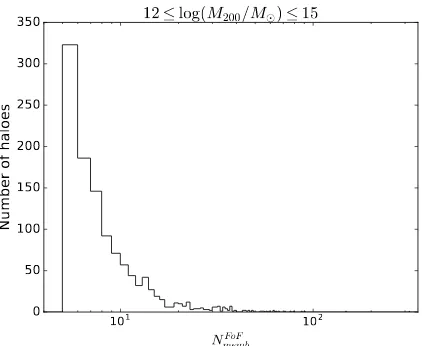
• At least 5 spectroscopically confirmed members identified by the FoF algorithm are needed to ob-tain reliable estimates of group properties such as velocity dispersion, halo mass and radius (Robotham et al. 2011). Figure 1 shows the his-togram of member galaxies in the halo sample.

101 ₁₀2 N_membFoF

0 50 100 150 200 250 300 350

Nu

mb

er

of

ha

loe

s

12 ≤ log(

M

/M

Figure 1. Number of haloes as a function of

spectro-scopically confirmed galaxies identified by the Friends-of-Friends algorithm (NFoF

memb). The histogram shows a peak atNmembFoF = 5.

galaxy groups with 1012 _{≤ (M}

200/M⊙) < 1014,

but we also include clusters with (M200/M⊙) ≥

1014 _{in order to compare the results for} low-mass halos with those for the high-low-mass ones. There is no known sharp mass cutoff that di-vides clusters and groups, but we assumeM200= 1014_M

⊙as a partition mass. M200is estimated us-ing the raw group velocity dispersions calculated by Robotham et al. (2011) and according to the

M200−σrelation ofMunari et al.(2013):

M200= σ3 10903_h(z)10

15_M

⊙ (1)

where h(z) = H(z)/(100 km s−1_Mpc−1_{) and} H(z) = H0pΩm(1 +z)3+ ΩΛ is the Hubble pa-rameter. We calculate the group radius R200 as the radius of a sphere with massM200.

2.3. Selection of member galaxies

The FoF algorithm tends to assign group member-ship to galaxies in the very central region of groups, out to∼1.5R200. However, we want to investigate the star formation in galaxies out to a projected distance of 9R200, and close to the group redshift. In this Section, we outline our method, which uses both galaxy redshifts and projected distance from the group center, as well as

M200, to extend the existing spectroscopically confirmed FoF group membership out to 9R200.

The reasons for probing such a large group-centric distance are twofold. First, we would like to compare our results with those ofRasmussen et al. (2012), who probed out to∼10R200. Second, analyzing out to such

large radii (i.e. > 4R200) means that we naturally in-clude a benchmark sample of field galaxies that are well beyond the regions where processes related to the group environment are expected to be important. This bench-mark sample will be drawn from the same redshift and galaxy stellar mass distributions as the group galaxies, and will therefore allow for an unbiased comparison to be made between the group galaxy properties and those of the benchmark field sample. One potential concern is that of stellar mass-segregation, which may lead to more massive galaxies being preferentially found close to the group center. However,Kafle et al. (2016) showed that there is negligible mass-segregation as a function of ra-dius in the GAMA groups out to 2R200.

In order to extend our study to 9R200, probing the group surroundings, we consider also galaxies in the same redshift range, but not assigned to groups by the FoF algorithm. We assign additional galaxies to groups in a manner similar toSmith et al.(2004), i.e. by min-imizing the C parameter as a function of redshift and projected location. Each additional galaxy is assigned only to one group and theC parameter is proportional to the logarithm of the probability that a galaxy is a member of a group assuming that the group velocity distribution is a Gaussian:

C= (czgal−czgroup)2/σ2−4 log(1−R/Rgroup) (2)

where c is the speed of light, σ is the group velocity dispersion,zgal andzgroupare the redshift of the galaxy and the group respectively, Ris the projected distance between the galaxy and the group center, and Rgroup is fixed at 9R200. The group center is estimated by Robotham et al.(2011) as the coordinates of the central galaxy defined with an iterative procedure.

In order to investigate low- and high-mass halos sep-arately and to perform a robust member selection, we define two samples according to their mass: groups with

M200/M⊙ = 1012−1014 and clusters withM200/M⊙=

1014₋₁₀15_{. For each sample we stack both FoF members} as well as the galaxies assigned to halos out to 9R200 and we calculate the infall velocities, i.e. the maximum allowed line-of-sight velocities for group/cluster galax-ies. We define only galaxies within these velocities as members. Figure2 shows the stacked PPS diagram in normalized units, i.e. Vrf/σ as a function of R/R200 where the galaxy rest-frame velocity is defined as:

Vrf =czgal−czgroup

(1 +zgroup) . (3)

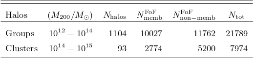
Table 1. Samples of galaxy groups and clusters.

Halos (M200/M⊙) Nhalos NmembFoF NnonFoF−memb Ntot

Groups 1012₋₁₀14 _{1104 10027 11762 21789}

Clusters 1014₋₁₀15 _{93 2774 5200 7974}

mass density profile (Navarro et al. 1996):

Vi(x) =

√

2Vc(x) (4)

where Vc is the circular velocity scaled by V200 = (GM200/R200)1/2 and given by:

_V c(R) V200

2

= 1

x

ln(1 +κx)−(κx)/(1 +κx)

ln(1 +κ)−κ/(1 +κ) . (5)

The concentration parameter κ is estimated according to the relation ofDolag et al.(2004) and depends on the medianz andM200of the group sample:

κ(M200, z) = κ0 1 +z

_M

200 1014_h−1_M

⊙ α

(6)

where κ0 = 9.59 and α =−0.102 for our cosmological model. The relationship between the concentration and the halo mass justifies our choice to determine the in-fall velocities for the two samples with different M200 ranges: we use z = 0.14, M200 = 1.5×1013M⊙ and z= 0.17,M200= 1.6×1014M⊙for groups and clusters,

respectively. In Figure 2 the different curves indicate the infall velocities for groups and clusters.

Table 1 lists the halo mass range of each sample (M200/M⊙), the number of halos (Nhalos), the number of members identified by the FoF algorithm (NFoF

memb), the number of galaxies not selected by the algorithm but assigned to a halo (NFoF

non−memb) and the resulting total number of members (Ntot).

Figure 3 shows the number of halos as a func-tion of redshift and halo mass. Groups and clusters show peaks at higher redshift because in that range a larger volume of targets has been probed. Most ha-los have 1013 _{≤ (M}

200/M⊙) ≤ 1014 and the majority

of member galaxies belong to these groups. In this context, this study represents a further step with re-spect to that of Oman & Hudson (2016), as well as of

von der Linden et al. (2010), since both of these works contain low-mass halos with masses < 1014_M

⊙, but

their satellite numbers are dominated by galaxies in clusters with mass≥1014_M

⊙, while we are probing the

group mass regime with the majority of galaxies.

2.4. Spectroscopic classification of galaxies

0 1 2 3 4 5 6 7 8 9

R/R200 −3

−2 −1 0 1 2 3

Vrf

/σ

12 ≤ log(M200/M⊙) ≤ 15 FoF members FoF non-members

Figure 2. Stacked PPS diagram used to select group/cluster

members. Red squares represent FoF members, whereas blue dots are for galaxies not selected by the algorithm but as-signed to a halo in order to probe radial distances out to 9R200. Black and green curves indicate the infall velocities for groups withM200/M⊙ = 1012−1014 and clusters with

M200/M⊙= 1014−1015, respectively.

Our primary aim in this paper is to investigate the properties of star-forming galaxies in groups. We select member galaxies with stellar mass 109 _{≤ (M}

∗/M⊙) ≤

1012to include both low- and high-mass galaxies and we identify the passive and star-forming populations. We consider only galaxies with a signal-to-noise ratio (S/N) per pixel greater than 3 in the 6383−6536 ˚A window.

Our spectroscopic classification is outlined below. First, we divide galaxies into two broad categories ac-cording to the features of their spectra: absorption- and emission-line galaxies. The absorption-line spectra are typical of galaxies dominated by an old and evolved stellar population, while emission-line galaxies can be characterized by young and new stars, by an AGN or by a Low-Ionization Nuclear Emission-line Region that have low levels of star formation activity and old stars. We use the convention of positive equivalent widths (EW) for emission lines and a negative sign for the absorption features. Since the Hα emission line is an excellent tracer of star formation, we use it to select emission-line galaxies. We follow Cid Fernandes et al.

(2011) and define emission-line galaxies as those having EW(Hα)>3˚A, and add the additional criteria that the S/N of the [NII] line must be larger than 3. The latter criterion helps to guard against spurious single line de-tections. Absorption-line galaxies are all the remaining ones with EW(Hα)≤3˚A (see Table2).

0.00 0.05 0.10 0.15 0.20 0.25

z

0 20 40 60 80 100 120 140 160

Nu

mb

er

of

ha

loe

s

12 ≤ log(M200/M⊙) < 14

14 ≤ log(M200/M⊙) ≤ 15

12.0 12.5 13.0 13.5 14.0 14.5 15.0

log(M200/M⊙)

0 50 100 150 200 250 300 350 400

Nu

mb

er

of

ha

loe

s

0 2000 4000 6000 8000 10000

Nu

mb

er

of

ga

lax

ies

Figure 3. Upper panel: Number of groups and clusters as

a function of z (dotted black and solid green lines, respec-tively). Lower panel: Number of halos and member galaxies as a function of M200 (solid black and dashed red lines, re-spectively). Most halos have 1013_≤(M

200/M⊙)≤1014 and the majority of member galaxies belong to these groups.

galaxies (Goto 2007;Paccagnella et al. 2017). However, the Hδ strong and post-starburst galaxies are < 1% and their inclusion does not affect our results. For the emission-line galaxies a further classification is needed to determine whether the emission is due to star forma-tion, since the EW(Hα) >3˚A cut does not necessarily imply that a galaxy is star-forming, as it includes AGN and composite systems. Thus, the emission-line galax-ies with S/N>3 of the Hβ, [OIII], Hαand [NII] lines are classified as star-forming or AGN according to the

Kauffmann et al.(2003) prescription, based on the flux ratios [NII]/Hαand [OIII]/Hβ:

log([OIII]/Hβ)≤ 0.61

log([NII]/Hα)−0.05+ 1.3 (7) We choose the Kauffmann et al.(2003) classification in order to avoid contamination by composite

galax-−2.0 −1.5 −1.0 −0.5 0.0 0.5 1.0

log

([NII]/H

)

−1.0 −0.5 0.0 0.5 1.0 1.5

log

([O

III]

/H

β

)

Star-forming

Composite

AGN

12 ≤ log(M200/M⊙) ≤ 15 Emission line galaxies

Figure 4. Stacked BPT diagram for emission-line

galax-ies with S/N> 3 of the Hβ, [OIII], Hα and [NII] lines (black triangles) to select star-forming galaxies. The red line represents the adopted star-forming/AGN classification of Kauffmann et al. (2003). The dashed green line shows the extreme-starburst model defined inKewley et al.(2001). Galaxies that fall in the region between the Kewley and Kauffmann lines are classified as composite galaxies.

ies. Prior to measuring the line ratios, the fluxes of the Balmer lines are corrected for the underlying stellar absorption in the following way (Hopkins et al. 2003):

FHλ=

EWHλ+ EWc EWHλ

fHλ (8)

where fHλ is the observed Hλ flux with λ = α or β, and EWc = 2.5˚A is the constant correction factor (Hopkins et al. 2013;Gordon et al. 2017). Figure4 dis-plays the BPT (Baldwin, Phillips, & Terlevich 1981) di-agram, i.e. log([OIII]/Hβ) versus log([NII]/Hα), used to identify star-forming galaxies and AGNs. There are 7990 galaxies where either Hα or Hβ or [OIII] had S/N<3. For those cases, we followCid Fernandes et al.

(2011) and define star-forming galaxies as those with log([NII]/Hα)≤ −0.4.

Table 2 summarizes the constraints for the spectro-scopic classification of member galaxies (Col. from 2 to 5) and reports their numbers (Col. 6).

2.5. SFR estimators

In this work we analyze whether and how the star formation activity is affected by the group/cluster en-vironment with respect to the field. We use two dif-ferent estimators of SFR taking advantage of the spec-troscopic and photometric GAMA data. The spectro-scopic estimator only probes the emission lines in the 2′′ _{aperture of the fiber and measures an}

Table 2. Spectroscopic classification of galaxies.

Spectral type EW Hα EW Hδ log([NII]/Hα) S/N [NII] Ngals ˚

A ˚A

Absorption ≤3 12000

Emission >3 >3 13500

Passive ≤3 ≥ −3 10663

Star-forming >3 ≤ −0.4 10239

AGN/Composite >3 >−0.4 3261

Note—There are 3 galaxies without measured EW(Hα) and 3 without measured EW(Hδ).

∼10 Myrs. The photometric SFR measurement includes light from the whole galaxy and is averaged over a longer timescale. Therefore, the two probes are complementary (see Davies et al. 2016bfor the details on scaling rela-tions).

The spectroscopic SFR (SFRHα) is calculated

assum-ing aSalpeter(1955) initial mass function:

SFRHα=

LHα

1.27×1034 (9)

where the Hα luminosity (LHα) is estimated

follow-ing the procedure outlined in Hopkins et al. (2003) and Gunawardhana et al. (2013). Briefly, the galaxy’s

r-band magnitude is used in combination with the fibre-based EW(Hα) to determine an approximately aperture-corrected, total LHα. A constant 2.5˚A is added

to EW(Hα) to account for stellar-absorption, and the Balmer decrement is used to correct for dust obscura-tion (seeGunawardhana et al. 2011,2013for a detailed explanation).

The photometric SFR (SFRMAGPHYS) is obtained with the spectral energy distribution (SED)-fitting code MAGPHYS (da Cunha et al. 2008; Davies et al. 2016b; Driver et al. 2016), which compares models of ultraviolet/optical/near-infrared spectral templates of stellar populations and mid-/far-infrared templates of dust emission with the observed photometry of a given galaxy, determining the overall best fit stellar+dust template. The MAGPHYS code provides an estimate of the galaxy SFR averaged over the last 100 Myr using a best-fitting energy balance model, where the obscuration-corrected SED is determined by balancing energy absorbed in the ultraviolet/optical with that emitted in the infrared.

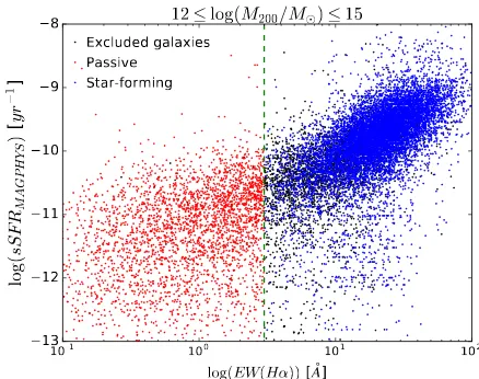
Both the spectroscopic and photometric SFR estima-tors are calculated for the star-forming galaxies spectro-scopically selected according to the procedure described in Section 2.4. We show in Figure5how the EW(Hα)>

3˚A cut affects the selection of star-forming galaxies and

10-1 ₁₀0 ₁₀1 ₁₀2

log(EW(Hα)) [Å] −13

−12 −11 −10 −9 −8

log(

sS

FR

M

AGP

HYS

)

[y

r

−

1]

12 ≤ log(M200/M⊙) ≤ 15 Excluded galaxies

Passive Star-forming

Figure 5. sSFRMAGPHYSas a function of EW(Hα) for the

whole galaxy population. The dashed green line represents the EW(Hα)>3˚A cut used to select star-forming galaxies (blue squares) from passive galaxies (red squares). Black squares represent excluded galaxies with EW(Hα) > 3˚A (EW(Hα) ≤ 3˚A ) and identified as AGN/composite (Hδ

strong/post-starburst).

maps into a limit in sSFR. We use sSFRMAGPHYSsince it is not possible to measure sSFRHαfor all galaxies.

3. ANALYSIS AND RESULTS

We explore how the group environment may affect galaxy star-forming properties. In order to pursue our aim we use two different samples of halos and galaxies, i.e. the Full Sample and the Restricted Sample. Their features are described below and are summarized in Ta-ble3:

• Full Sample: this includes all the halos at 0.05≤

z≤0.2 and galaxies with 109_≤(M

∗/M⊙)≤1012

out to 9R200 (see Sections 2.2−2.4).

Full Sample. It includes halos at 0.05≤z≤0.15 and galaxies with 1010_≤(M

∗/M⊙)≤1012out to

9R200. The chosen z and M∗ limits correspond

to a completeness of∼95% according to Figure 6 of Taylor et al.(2011) (the grey line refers to our galaxy sample observed down to r < 19.8 mag), who estimated the GAMA stellar mass complete-ness limit as a function of redshift.

We perform the following analyses using the Full Sam-ple and the Restricted SamSam-ple in the Sections listed in Table3 for the following reasons:

• In Sections 3.1 and 3.2 we compare the fractions of passive (PAS) and star-forming (SF) galax-ies in radial and projected-phase spaces, respec-tively. We use the Restricted Sample. The stellar mass cut is necessary because we measure frac-tions for different galaxy populafrac-tions, i.e passive fraction and star-forming fraction. At a given r -band magnitude, blue star-forming galaxies have a lower stellar mass when compared with red pas-sive galaxies. Therefore, probing a galaxy stellar mass range that is not complete would bias against passive galaxies for a given stellar mass, and affect the measured fractions.

• In Section 3.3 we investigate the distribution of the passive and star-forming populations in velocity space. We use the Full Sample, without taking into account the stellar mass completeness limit since we are not studying galaxy fractions.

• In Sections 3.4−3.8 we focus only on star-forming galaxies of the Full Sample and study the de-pendence of star formation rate (SFR) on group-centric radius and galaxy stellar mass.

Table 3. Full and Restricted Samples of halos and galaxies.

Full Restricted

Nhalos 1197 679

z 0.05−0.20 0.05−0.15

(M200/M⊙) 1012−1015 1012−1015

(M∗/M⊙) 109₋₁₀12 ₁₀10₋₁₀12

Sections 3.3−3.6 3.1−3.2

3.1. Fractions of galaxies in radial space

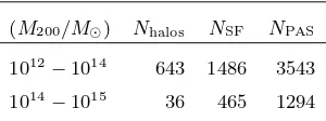
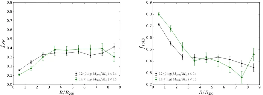
Different works confirm that group galaxy properties such as morphology, color and spectral type all cor-relate with group-centric distance (e.g., Carlberg et al. 2001;Tran et al. 2001;Girardi et al. 2003;Wetzel et al. 2012;Hou et al. 2014). In order to test the presence of the passive versus star-forming−radius relation, we con-sider the Restricted Sample and explore the fractions of star-forming and passive galaxies as a function of group-centric radius in Figure 6. The fraction of each galaxy population is estimated with respect to the total galaxy sample containing passive, Hδ strong, post-starburst, star-forming galaxies and AGNs/composites. Table 4

lists the numbers of halos (Nhalos), star-forming (NSF) and passive (NPAS) galaxies for eachM200range.

Figure 6 shows that the fraction of passive galax-ies strongly decreases from the inner halo regions to ∼ 3.5R200 in clusters and ∼ 2.5R200 in groups (right

panel), while the fraction of star-forming galaxies

in-creases out to the same radii (left panel). Beyond these distances both the fractions remain approximately con-stant. In groups the passive fraction declines by a factor ∼ 2 at 2.5R200, while the star-forming fraction rises by a factor ∼ 1.5 at the same radius. The max-imum is fSF ∼ 0.40 at 9R200 because of the selected range in stellar mass 1010 _{≤ (M}

∗/M⊙) ≤ 1012 and

there are fewer star-forming objects with higher mass (Taylor et al. 2015). Our results confirm that the pas-sive versus star-forming−radius relation is present in galaxy groups as well as in the more studied cluster environment and that star-forming galaxies are mainly found in the halo outskirts, in agreement with previ-ous works (e.g.,Whitmore et al. 1993;Tran et al. 2001;

Girardi et al. 2003;Goto et al. 2003;Brough et al. 2006;

Wetzel et al. 2012;Hou et al. 2014;Fasano et al. 2015).

Table 4. Restricted Sample: galaxy populations out to

9R200.

(M200/M⊙) Nhalos NSF NPAS

1012₋₁₀14 _{643 1486 3543}

1014₋₁₀15 _{36 465 1294}

3.2. Fractions of galaxies in projected phase space

0 1 2 3 4 5 6 7 8 9 R/R200

0.0 0.1 0.2 0.3 0.4 0.5 0.6 0.7 0.8 0.9

fSF

12 ≤ log(M200/M⊙) < 14

14 ≤ log(M200/M⊙) ≤ 15

0 1 2 3 4 5 6 7 8 9

R/R200 0.2

0.3 0.4 0.5 0.6 0.7 0.8 0.9

fPAS

12 ≤ log(M200/M⊙) < 14

14 ≤ log(M200/M⊙) ≤ 15

Figure 6. Fractions of star-forming (left panel) and passive galaxies (right panel) as a function of projected radius for groups (black dots) and clusters (green diamonds). We consider 9 radial bins and binomial error bars. The fraction of passive galaxies strongly decreases from the inner halo regions to large radii, while the fraction of star-forming galaxies increases towards the outskirts.

Jaff´e et al. 2015), and for samples with both cluster and group mass halos (Oman et al. 2013; Oman & Hudson 2016). Our GAMA sample allows us to probe the group halo mass range alone (1012_≤(M

200/M⊙)<1014) with

a larger number of galaxies and to determine whether the segregation of star-forming and passive galaxies ob-served in the PPS of clusters also exists in groups.

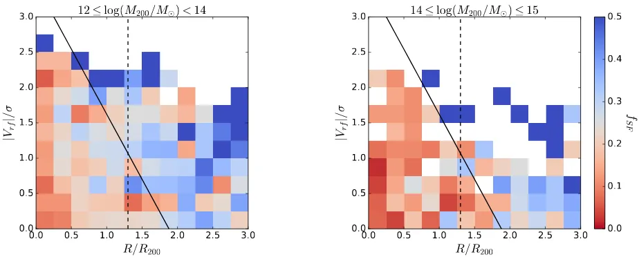
We use the Restricted Sample and Figure7shows the 2D histograms of star-forming fractions binned in the PPS. We consider the radial range out to 3R200 in or-der to study a region containing galaxies which can be or have been physically affected by the group/cluster environment. We plot the separation line (solid black) between the region that are likely to have a high fraction of recently accreted galaxies (i.e., the infalling popula-tion) and the region with galaxies that have been inside the group/cluster for an extended period of time (i.e., the virialized population), found byOman et al.(2013) for simulated groups and clusters. We adapt the galaxy velocity−radius relation ofOman et al.(2013) to:

|Vrf|

σ =−

4 3

1 1.25

R R200

√

3 + 2√3 (10)

where the factors of√3 and 1.25 convert from the 3D velocity dispersion σ3D and the virial radius Rvir used by Oman et al.(2013) to our 1D σand R200, i.e. σ = σ3D/

√

3 and Rvir = 1.25R200 1 at z= 0. We also plot the separation line (dashed black) between the virialized and infalling populations established byMahajan et al.

(2011) atR∼1.3R200.

1_{In the relation}R_{vir= 1}.₂₅R_{200the value 1.25 does not} com-pare in Oman et al. (2013), but it has been provided to us via private communication from Mike Hudson.

The virialized region at small radii is characterized by low values of fSF and it is most populated by pas-sive galaxies, whereas for the infalling region at large distances the fraction of star-forming galaxies is higher. This result is observed for both groups and clusters. We conclude that the segregation of star-forming and pas-sive galaxies in the PPS already detected in clusters and in combined group and cluster samples is also observable in low-mass halos alone.

3.3. Segregation in velocity space

The analysis of the star-forming and passive fractions in the radial space reveals a segregation of the two galaxy populations in both groups and clusters. However, pre-vious works focusing on clusters also observed galaxy color/spectral type and luminosity segregation when considering velocity space alone (e.g., Biviano et al. 1992, 1997; Adami et al. 1998; Ribeiro et al. 2013;

Haines et al. 2015; Barsanti et al. 2016). These ef-fects have been also detected in groups, but are less studied (e.g., Girardi et al. 2003; Lares et al. 2004;

Ribeiro et al. 2010).

star-0.0 0.5 1.0 1.5 2.0 2.5 3.0

R/R200 0.0

0.5 1.0 1.5 2.0 2.5 3.0

|Vrf

|/σ

12 ≤ log(M200/M⊙) < 14

0.0 0.5 1.0 1.5 2.0 2.5 3.0

R/R200 0.0

0.5 1.0 1.5 2.0 2.5 3.0

|Vrf

|/σ

14 ≤ log(M200/M⊙) ≤ 15

0.0 0.1 0.2 0.3 0.4 0.5

f

SF

Figure 7. 2D histograms of star-forming galaxy fractions binned in the PPS for groups and clusters. The virialized region at

small radii is characterized by low values offSF (redder colors) and it is most populated by passive galaxies, whereas for the infalling region at large distances the fraction of star-forming galaxies is higher (bluer colors). The solid and dashed black lines represent the separation between the virialized and infalling galaxy populations found byOman et al.(2013) andMahajan et al. (2011), respectively.

forming and 5203 (1882) passive galaxies within 1.5R200 are different at the≥99.99% confidence level (c.l.). We confirm the segregation of the passive and star-forming populations in the velocity space at both the group and cluster mass regimes.

Finally, we explore a possible galaxy stellar mass seg-regation in velocity space, since Kafle et al. (2016) ob-served noM∗ segregation with radius for GAMA group

galaxies. We use the Full Sample and plot in Fig-ure 9 the median |Vrf|/σ versus M∗ for star-forming

and passive galaxies of groups and clusters. We re-strict this analysis within 1R200 since this segregation is likely associated to secondary relaxation processes within the halo virialized regions (Binney & Tremaine 2008). From the GAMA halos of the Full Sample we exclude the central galaxies which have been defined by

Robotham et al. (2011). The inclusion of these galax-ies could potentially bias our results. The selection of Robotham et al.(2011) is generally robust, but it is based on an iterative procedure and it is possible that this method chooses the incorrect central galaxy, thus there may be some contamination.

Massive passive galaxies show evidence of segrega-tion in the velocity space: more massive galaxies have lower |Vrf|/σ values than the low-mass ones. However, this effect does not appear to be a statistically sig-nificant result for massive star-forming galaxies likely due to the low numbers of these galaxies with highM∗

(Taylor et al. 2015). For both the galaxy populations in groups, the trend in velocity remains approximately constant for galaxies with 109 _{≤ (M}

∗/M⊙) < 1010.7

and then it decreases for 1010.7 _{≤ (M}

∗/M⊙) ≤ 1012.

For clusters the velocity decline starts at about M∗ ≥

1011.2_M

⊙ and M∗ ≥ 1010.7M⊙ for passive and

star-forming galaxies, respectively. To statistically evalu-ate this segregation, we apply the Spearman test in order to estimate the correlation between |Vrf|/σ and M∗ for galaxies with a flat trend and for those with a

decline in velocity separately. Tables 5 reports the P -values for star-forming and passive galaxies in eachM200 range. Massive passive galaxies have smaller P-values implying a strong segregation. On the other hand, only the massive star-forming galaxies in clusters present a marginally statistically significant decrease in velocity. Finally, for both the galaxy populations low-mass galax-ies do not show a correlation between |Vrf|/σ and M∗

and have a flat trend in velocity.

These results are in agreement with a scenario where the dynamical friction mechanism is able to slow the orbital motion of galaxies in groups and clusters (Biviano et al. 1992; Adami et al. 1998; Girardi et al. 2003; Ribeiro et al. 2010, 2013; Barsanti et al. 2016). In agreement with the previous works, we confirm that this deceleration is a function of galaxy mass: for more massive galaxies, the higher the deceleration. We also observe that this segregation is stronger for passive galaxies than for star-forming galaxies.

3.4. SFR−radius relation for star-forming galaxies

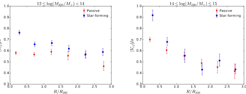
0.0 0.5 1.0 1.5 2.0 2.5 3.0

R/R200

0.3 0.4 0.5 0.6 0.7 0.8 0.9 1.0

|

Vrf

|/

σ

12 ≤ log(M200/M⊙) < 14

Passive Star-forming

0.0 0.5 1.0 1.5 2.0 2.5 3.0

R/R200

0.3 0.4 0.5 0.6 0.7 0.8 0.9 1.0

|

Vrf

|/

σ

14 ≤ log(M200/M⊙) ≤ 15

Passive Star-forming

Figure 8. |Vrf|/σ versusR/R200 for star-forming and passive galaxies within 3R200 in groups and clusters. We plot median

values in 6 radial bins and bootstrap errors at 68% c.l.; the abscissa points are set to the biweight mean of theR/R200distribution within the bin of interest. Star-forming galaxies within 1.5R200 have higher |Vrf|/σ values when compared with the passive galaxy population.

9.0 9.5 10.0 10.5 11.0 11.5 12.0

log(M∗/M)

0.1 0.2 0.3 0.4 0.5 0.6 0.7 0.8 0.9 1.0

|

Vrf

|/

σ

12 ⊙ log(M200/M) < 14

Passive Star-forming

9.0 9.5 10.0 10.5 11.0 11.5 12.0

log(M∗/M)

0.1 0.2 0.3 0.4 0.5 0.6 0.7 0.8 0.9 1.0

|

Vrf

|/

σ

14 ⊙ log(M200/M) ⊙ 15

Passive Star-forming

Figure 9. |Vrf|/σversusM∗for star-forming and passive galaxies within 1R200 in groups and clusters. We plot median values in 6 bins and bootstrap errors at 68% c.l.; the abscissa points are set to the biweight mean of theM∗distribution within the bin of interest. More massive galaxies have lower|Vrf|/σvalues than the low-mass ones which show a constant trend in velocity.

well established for star-forming cluster galaxies which also show suppressed star formation with respect to the field (e.g., Lewis et al. 2002; G´omez et al. 2003;

von der Linden et al. 2010; Paccagnella et al. 2016). However, this latter observation is less clear for star-forming galaxies in groups. In the Sections 3.4−3.8 we explore whether and how the group environment affects the star formation properties, analyzing the dependence of SFR on radius and stellar mass.

We focus on star-forming galaxies of the Full Sam-ple within 9R200, probing a similar stellar mass and radial range as Rasmussen et al. (2012) and including a benchmark sample of field galaxies (see Section 2.3). The star-forming galaxies are spectroscopically selected as described in the Section 2.4. For these galaxies we define in the Section 2.5 two different SFR estimators, i.e. SFRHα and SFRMAGPHYS, based on the spectro-scopic and photometric properties of galaxies,

respec-tively. Table 6 lists the number of star-forming galax-ies with available SFRHαand SFRMAGPHYS. There are fewer star-forming galaxies with measured SFRHαwhen

compared with those with available SFRMAGPHYS: 460 galaxies have no measured SFRHαbecause their spectra

are not flux calibrated and/or it is not possible to make obscuration corrections.

Figure10shows median SFRHαvalues versusR/R200 for star-forming galaxies associated to groups and clus-ters. For clusters the SFRHα remains constant over

2.5 < (R/R200) ≤ 9 and then decreases towards the cluster center. For groups there is a continuous decrease of the star formation activity from the group outskirts to the inner regions. The shift towards higher SFRHα

Table 5.Spearman test.

(M200/M⊙) Type log(M∗/M⊙) Ngals P

1012₋₁₀14 _{PAS 9.0−10.7 2596 0.6533}

1012₋₁₀14 _{PAS 10.7−12.0 1942 0.0004}

1012−1014 SF 9.0−10.7 1942 0.1260

1012₋₁₀14 _{SF 10.7−12.0 111 0.6689}

1014−1015 PAS 9.0−11.2 1031 0.8876

1014₋₁₀15 _{PAS 11.2−12.0 604 0.0313}

1014₋₁₀15 _{SF 9.0−10.7 462 0.1312}

1014−1015 SF 10.7−12.0 12 0.0513

Note—P-values quantifying the correlation between |Vrf|/σandM∗for passive and star-forming galaxies in

groups/clusters.

Table 6. Full Sample: star-forming galaxies out to 9R200.

(M200/M⊙) NSFR,Hα NSFR,MAGPHYS

1012₋₁₀14 _{7213 7568}

1014₋₁₀15 _{2565 2670}

0 1 2 3 4 5 6 7 8 9

R/R200 −0.1

0.0 0.1 0.2 0.3 0.4

log(

SFR

Hα

)

[M

⊙

/y

r]

12 ≤ log(M200/M⊙) < 14

14 ≤ log(M200/M⊙) ≤ 15

Figure 10. SFRHαas a function of projected

group/cluster-centric distance for star-forming galaxies. We plot median values binned every 1R200with errors at the 68% c.l. There is a decline of SFRHαtowards the halo inner regions.

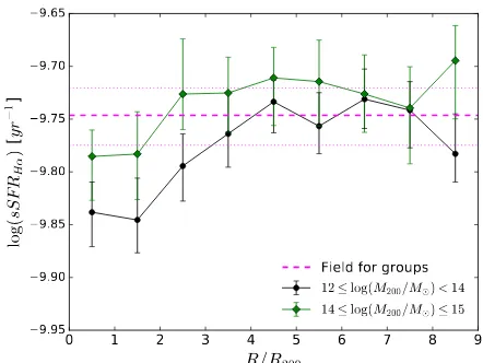
We also analyze the dependence of specific star for-mation rate (sSFR=SFR/M∗) on radius. Figure 11

confirms the decline of SFRHα at ∼ 2.5R200 towards the cluster centers and it shows a drop in sSFRHα at

∼4.5R200 for star-forming galaxies in groups, which is

0 1 2 3 4 5 6 7 8 9

R/R200 −9.95

−9.90 −9.85 −9.80 −9.75 −9.70 −9.65

log(

sS

FR

Hα

)

[y

r

−

1]

Field for groups 12 ≤ log(M200/M⊙) < 14

14 ≤ log(M200/M⊙) ≤ 15

Figure 11. sSFRHα as a function of projected

group/cluster-centric distance for star-forming galaxies. The dashed magenta line indicates the median sSFRHαfor galax-ies associated to groups but outside 4.5R200 and defined as belonging to the field, with the dotted magenta lines marking the uncertainties on that. The sSFRHα declines by a factor

∼1.2 from the field to the group inner region.

not evident in Figure 10 where there is a continuous decline. In order to compare the star formation in the group environment with that in the field, we consider star-forming galaxies atR≤4.5R200as group members and those with R > 4.5R200 as field galaxies. Com-paring the median sSFRHα value for the field (magenta

line) with that for star-forming group galaxies in the 0≤(R/R200)<1 bin (black point), it can be seen that the sSFRHα declines by a factor of∼1.2. These results

are in agreement with the outcome ofRasmussen et al.

(2012), who found a decrease in the sSFR as a function of the projected group-centric distance for star-forming galaxies in nearby groups.

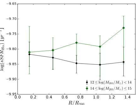
In order to compare our analysis with that of

Ziparo et al. (2013), we consider galaxies only out to 1.5R200in Figure12, sinceZiparo et al.(2013) investi-gated the SFR− and sSFR−radius relation within this radial distance. Figure 12 shows that there is no sta-tistically significant correlation between sSFRHα and R/R200 at small radii for groups, but the uncertainties are large. This results agrees withZiparo et al.(2013).

0.0 0.2 0.4 0.6 0.8 1.0 1.2 1.4 R/R200

−9.95 −9.90 −9.85 −9.80 −9.75 −9.70 −9.65

log(

sS

FR

Hα

)

[y

r

−

1]

12 ≤ log(M200/M⊙) < 14

14 ≤ log(M200/M⊙) ≤ 15

Figure 12. sSFRHαversusR/R200for star-forming galaxies

out to 1.5R200in groups and clusters. There is no change of sSFRHαwith radius.

suppression is too slow to be detected at small radii. As a consequence, the quenching timescale probably is of the order of few Gyr and comparable to the group crossing time. This result is in agreement with the con-clusion ofvon der Linden et al.(2010), who proposed a scenario in which star formation is quenched slowly.

Finally, we explore the dependence of SFRMAGPHYS and sSFRMAGPHYSon projected group-centric radius for star-forming galaxies in Figure13. Theleft panelshows for clusters a continuous decrease in SFRMAGPHYS to-wards the cluster center, whereas for groups there is a drop at ∼ 2.5R200. The decline in star forma-tion is more evident in the right panel which illus-trates a decreasing trend in sSFRMAGPHYSat∼3.5R200 for both groups and clusters. Comparing the median sSFRMAGPHYS value for star-forming group galaxies in the 0 ≤(R/R200) < 1 bin (black point) with that for the associated field galaxies at 4.5<(R/R200)≤9 (ma-genta line), it can be seen that the sSFRMAGPHYS de-clines by a factor of ∼ 1.5 from the field to the group inner region. The results obtained using the SED-fitting code MAGPHYS as a star formation estimator are in agreement with those based on the Hα emission lines within the uncertainties.

Throughout the different analyses of this Section we have used three different radial limits, i.e. 1.5R200, 4.5R200, and 9R200. The primary motivation behind selecting these limits was to allow us to compare with previous studies such as Rasmussen et al. (2012) and

Ziparo et al. (2013). However, these radial limits may also be interpreted in a more physical manner. The region R ≤1.5R200 is where a large fraction of galax-ies that have encountered the group/cluster core reside

(Gill et al. 2005; Mahajan et al. 2011), and where we observe the strongest signature of suppressed star for-mation. The range 1.5 ≤ (R/R200) < 4.5 is the re-gion containing bound populations that may infall onto the group/cluster, in agreement withRines et al.(2013) who found that the maximum radius enclosing gravi-tationally bound galaxies to the halo is at 4−5R200. This region is mainly populated by star-forming galax-ies. Finally, beyond 4.5R200 there is the unbound field population.

In conclusion, a decline is observed in star formation activity with decreasing group-centric radius for star-forming galaxies. The radius at which this decline be-gins differs for the various measures of SFR and for the different halo mass ranges probed. Generally, the decline begins in the radial range 2.5 ≤(R/R200) ≤4.5. This distance is well beyond the radius at which the group environment is expected to play a role in quenching star formation, and is also beyond the apocentric distance to which a galaxy will travel after its first passage of the group (Gill et al. 2005). Thus, this may indicate that galaxies are being pre-processed in very low-mass groups not detected in the GAMA catalog, or in the fil-ament environment (e.g.,Alpaslan et al. 2016), prior to falling into the GAMA-identified halos. However, many factors can conspire to spread the point at which the SFR decline starts out in radius. For example, uncer-tainties in the estimate ofR200are likely to be relatively high due to the propagation of the errors in the velocity dispersion/mass measurements used to define the R200 values. These uncertainties will broaden any sharp de-cline in radius.

3.5. sSFR histograms

The sSFRHα−radius relationship in Figure11 shows

that for groups the median sSFRHα declines with

ra-dius towards the group center, but is relatively flat for

R > 4.5R200. This behavior at large radius is to be expected, since galaxies at these radii are too distant to have been affected by the group environment, and are highly unlikely to have traversed the group. Thus, we use the star-forming galaxies with R > 4.5R200 as a benchmark field sample for comparison to group mem-ber galaxies at 0≤(R/R200)≤4.5.

0 1 2 3 4 5 6 7 8 9

R/R200

−0.1 0.0 0.1 0.2 0.3 0.4

log(

SFR

M

AG

PHY

S

)

[M

⊙

/y

r]

12 ≤ log(M200/M⊙) < 14

14 ≤ log(M200/M⊙) ≤ 15

0 1 2 3 4 5 6 7 8 9

R/R200

−9.95 −9.90 −9.85 −9.80 −9.75 −9.70 −9.65 −9.60

log(

sS

FR

M

AG

PHYS

)

[y

r

−

1]

Field for groups

12 ≤ log(M200/M⊙) < 14

14 ≤ log(M200/M⊙) ≤ 15

Figure 13. SFRMAGPHYS and sSFRMAGPHYS versusR/R200 for star-forming galaxies (left and right panel, respectively) in

groups and clusters. We plot median values binned every 1R200 with errors at the 68% c.l. The dashed magenta line indicates the median sSFRMAGPHYS for galaxies associated to groups but outside 4.5R200 and defined as belonging to the field, with the dotted magenta lines marking the uncertainties on that. There is a decline in star formation with decreasing radius and sSFRMAGPHYSdeclines by a factor∼1.5 from the field to the group inner region.

mass relationship with SFR and since we are interested in comparing measurements of star formation from the last∼10 Myrs. We analyze sSFR histograms since the median distills a lot of information about the distribu-tions of the sSFRs at a given radius into one point. The median of the sSFR distribution of group galaxies can be different with respect to that of field galaxies because there can be an overall shift in the total distribution of groups with respect to the field. However, another rea-son is that the sSFR distribution of groups can have a significant asymmetry, or bi-modality, that produces a difference in the medians. Investigating the sSFR his-tograms, we explore if there is a difference of the sSFR distribution in groups with respect to that in the field and we try to understand which of the above reasons for different medians is the case. Discerning between these two causes is important because it may give clues about the mechanisms responsible for the sSFR quenching.

We consider the Full Sample. Group/cluster members are defined as galaxies with 0 ≤ (R/R200) ≤ 4.5 and havingVrf lower or equal to the infall velocities (see Fig-ure2). We build the field as populated by galaxies with 4.5 < (R/R200) ≤ 9 in and outside the curves repre-senting the infall velocities, i.e. with−5≤(Vrf/σ)≤5, in order to obtain a statistically high number of field galaxies. Moreover, each field galaxy is assigned to a halo according to the procedure of Smith et al. (2004) described in Section 2.3. We produce two separate field samples for each of the M200 range. Finally, the star-forming galaxy population in each field is selected by applying the same method described in Section 2.5 and used to define star-forming members. The numbers of star-forming group and cluster galaxies in each radial bin and in the respective field are reported in Table7.

We apply the Kolmogorov−Smirnov test (K−S test;

Table 7. Full Sample: star-forming galaxies in radial bins.

(M200/M⊙) (R/R200) Ngals

Groups 1012₋₁₀14 _{0.0−1.0 1945}

Groups 1012₋₁₀14 _{1.0−2.0 1068}

Groups 1012−1014 2.0−4.5 1677

Field 1012₋₁₀14 _{4.5−9.0 4177}

Clusters 1014−1015 0.0−1.0 446

Clusters 1014₋₁₀15 _{1.0−2.0 273}

Clusters 1014₋₁₀15 _{2.0−4.5 752}

Field 1014−1015 4.5−9.0 2390

However, the K−S test does not probe differences in the tails of the distributions, but it is more sensitive to the behavior of the distributions close to their median values. Thus, following the procedure ofZabludoff et al.

(1993) andOwers et al.(2009), the sSFR distribution is approximated by a series of Gauss-Hermite functions up to order 4 and we estimate the strength of the asymmet-ric and symmetasymmet-ric departures from a Gaussian shape. Figures14and15show the log(sSFRHα) histograms for

the group/cluster star-forming galaxies in different ra-dial ranges and in the respective field reported in Ta-ble7, and they list the mean value (<log(sSFRHα)>),

standard deviation (σlog(sSFRHα)), skewness (h3) and kurtosis (h4) with the respective P-values showing the significance of these terms (P[h3] and P[h4]). The group/cluster sSFR distributions are characterized by larger σlog(sSFRHα) and lower< log(sSFRHα) > values compared to the associated field. Moreover, the group sSFR histograms in the radial ranges 0≤(R/R200)<1 and 1 ≤ (R/R200) < 2 show significant evidence for asymmetry, withh3=−0.054 for both, meaning heavier tails for the lower sSFR side of the distribution relative to a Gaussian shape. This indicates a galaxy popula-tion with suppressed sSFR in groups. We do not find significant skewness values for the cluster sSFR distri-butions likely because of the smaller number of clusters and galaxies therein.

3.6. SFR₋galaxy stellar mass relationship

Since the comparison between the sSFR distributions of star-forming group/cluster and field galaxies indicates that the median sSFRs are lower in groups/clusters than in the field, we compare the SFR−M∗

relation-ship for group and cluster members with that for the respective field in order to check whether and how this relation changes with environment. We also analyze whether the SFR quenching is stronger for

Table 8. K−S test.

(M200/M⊙) (R/R200) P

1012−1014 0.0−1.0 6.76×10−16 1012₋₁₀14 _{1.0−2.0 7.36×10}−11 1012₋₁₀14 _{2.0−4.5 1.95×10}−2 1012−1014 0.0−4.5 5.72×10−15 1014₋₁₀15 _{0.0−1.0 1.47×10}−4 1014−1015 1.0−2.0 5.59×10−2 1014₋₁₀15 _{2.0−4.5 7.79×10}−1 1014₋₁₀15 _{0.0−4.5 1.34×10}−2

Note—P-values from comparing the group/cluster sSFR distribution binned in radius with that of the respective

field.

low-mass galaxies compared with the high-mass ones, since this effect has been found by several studies (e.g.,von der Linden et al. 2010;Rasmussen et al. 2012;

Davies et al. 2016a; Schaefer et al. 2016).

Figure 16shows SFRHαas a function ofM∗ for

star-forming members of the Full Sample in different ra-dial ranges out to 4.5R200, respectively of groups and clusters, and for the assigned field galaxies at 4.5 <

(R/R200)≤9 according to the result of Figure11. The numbers of galaxies for each range inM200andR200are reported in Table7. We plot the median SFR−M∗

re-lations binning galaxies with 109 ≤(M∗/M⊙)≤1011.5

in 5 bins, since the range 1011.5_<(M

∗/M⊙)≤1012 is

populated by too few galaxies. In all cases the SFR goes up as M∗ increases, forming the well known and often

named star formation main sequence (Daddi et al. 2007;

Noeske et al. 2007).

At fixed stellar mass, star-forming group/cluster members are shifted towards lower median values of SFRHα when compared with the values of the

respec-tive field galaxies. This means that there is a galaxy population with suppressed star formation activity in groups/clusters which is less noticeable in the field.

The difference between the median SFRHα of

clus-ter members and field galaxies becomes less visible as the radial range is closer to the field and for the range 2 ≤ (R/R200) ≤ 4.5 there is no shift between the SFR−M∗ relationships in the cluster and field

galax-0 < R/R200 < 1

-12 -11 -10 -9 -8

log(sSFR) 0.00

0.05 0.10 0.15

Fraction of galaxies

0 < R/R200 < 1

-12 -11 -10 -9 -8

log(sSFR) 0.00

0.05 0.10 0.15

Fraction of galaxies

<log(sSFR)>=-9.83 σlog(sSFR)=0.51

h3=-0.054, P[h3]=0.00

h4=0.016, P[h4]=0.24

N=1945

1 < R/R200 < 2

-12 -11 -10 -9 -8

log(sSFR) 0.00

0.05 0.10 0.15

Fraction of galaxies

1 < R/R200 < 2

-12 -11 -10 -9 -8

log(sSFR) 0.00

0.05 0.10 0.15

Fraction of galaxies

<log(sSFR)>=-9.84 σlog(sSFR)=0.51

h3=-0.054, P[h3]=0.01

h4=-0.020, P[h4]=0.25

N=1068

2 < R/R₂₀₀ < 4.5

-12 -11 -10 -9 -8

log(sSFR) 0.00

0.05 0.10 0.15 0.20

Fraction of galaxies

2 < R/R₂₀₀ < 4.5

-12 -11 -10 -9 -8

log(sSFR) 0.00

0.05 0.10 0.15 0.20

Fraction of galaxies

<log(sSFR)>=-9.77 σlog(sSFR)=0.44

h3=-0.008, P[h3]=0.63

h4=0.033, P[h4]=0.06

N=1677

R/R₂₀₀ > 4.5

-12 -11 -10 -9 -8

log(sSFR) 0.00

0.05 0.10 0.15 0.20

Fraction of galaxies

R/R₂₀₀ > 4.5

-12 -11 -10 -9 -8

log(sSFR) 0.00

0.05 0.10 0.15 0.20

Fraction of galaxies

<log(sSFR)>=-9.74 σlog(sSFR)=0.42

h3=0.014, P[h3]=0.14

h4=0.031, P[h4]=0.01

N=4177

Figure 14. log(sSFRHα) histograms for the group star-forming galaxies in different radial ranges and in the respective

field (black line), approximated by a series of Gauss-Hermite functions up to order 4 (red line) to estimate the asymmetric and symmetric departures from a Gaussian shape (blue line). The group log(sSFRHα) distributions are compared with the respective field one (green line), showing larger σlog(sSFRHα) and lower<log(sSFRHα)>values than the field. The group histograms in the radial ranges 0≤(R/R200)<1 and 1≤(R/R200)<2 show significant evidence for asymmetry towards the lower sSFRHα side of the distribution relative to a Gaussian shape.

ies in 31 OMEGAWINGS clusters at 0.04 < z < 0.07 with that of the field, considering only galaxies with

M∗ >109.8M⊙. They found a population of quenched

star-forming galaxies in these clusters that is rare in the field, suggesting that the transition from star-forming to passive occurs on a sufficiently long timescale to be observed. However,Paccagnella et al.(2016) observed a more evident transition galaxy population with respect to our result, likely due to the fact that their sample contains many more cluster galaxies than ours, i.e. 9242 and 1546 cluster galaxies in total, respectively.

We do not find a stronger suppression in SFR for low-mass galaxies in both groups and clusters, but the shift in SFR occurs over the whole range in M∗. Rasmussen et al.(2012) found that the SFR suppression is strongest for low-mass galaxies with M∗ ≤ 109M⊙,

while the decline is negligible for high-mass galaxies with

M∗ > 1010M⊙. They detected a dependence of the

sSFR−radius relation on M∗ that we do not observed

in our data. However, we do not probe galaxies with

M∗ ≤109M⊙ as Rasmussen et al.(2012), and a future

inclusion of these galaxies could be crucial for shedding light on this effect.

Finally, we consider the photometric estimators of the star formation activity, plotting median values of SFRMAGPHYSinM∗bins, in order to compare these

re-sults with those obtained using SFRHα. We use

star-forming galaxies with available SFRMAGPHYS in the same radial and halo mass ranges as in the previous case and in the respective field. Figures17shows that there is a change of the SFR−M∗ relation with the

0 < R/R200 < 1

-12 -11 -10 -9 -8

log(sSFR) 0.00

0.05 0.10 0.15

Fraction of galaxies

0 < R/R200 < 1

-12 -11 -10 -9 -8

log(sSFR) 0.00

0.05 0.10 0.15

Fraction of galaxies

<log(sSFR)>=-9.81 σlog(sSFR)=0.52

h3=-0.011, P[h3]=0.76

h4=0.021, P[h4]=0.50

N=446

1 < R/R200 < 2

-12 -11 -10 -9 -8

log(sSFR) 0.00

0.05 0.10 0.15 0.20

Fraction of galaxies

1 < R/R200 < 2

-12 -11 -10 -9 -8

log(sSFR) 0.00

0.05 0.10 0.15 0.20

Fraction of galaxies

<log(sSFR)>=-9.78 σlog(sSFR)=0.44

h3=-0.039, P[h3]=0.36

h4=0.081, P[h4]=0.04

N=273

2 < R/R₂₀₀ < 4.5

-12 -11 -10 -9 -8

log(sSFR) 0.00

0.05 0.10 0.15 0.20

Fraction of galaxies

2 < R/R₂₀₀ < 4.5

-12 -11 -10 -9 -8

log(sSFR) 0.00

0.05 0.10 0.15 0.20

Fraction of galaxies

<log(sSFR)>=-9.70 σlog(sSFR)=0.47

h3=-0.027, P[h3]=0.28

h4=0.000, P[h4]=0.98

N=752

R/R₂₀₀ > 4.5

-12 -11 -10 -9 -8

log(sSFR) 0.00

0.05 0.10 0.15 0.20

Fraction of galaxies

R/R₂₀₀ > 4.5

-12 -11 -10 -9 -8

log(sSFR) 0.00

0.05 0.10 0.15 0.20

Fraction of galaxies

<log(sSFR)>=-9.72 σlog(sSFR)=0.45

h3=0.003, P[h3]=0.86

h4=-0.001, P[h4]=0.96

N=2390

Figure 15. log(sSFRHα) histograms for the cluster star-forming galaxies in different radial ranges and in the respective

field (black line), approximated by a series of Gauss-Hermite functions up to order 4 (red line) to estimate the asymmetric and symmetric departures from a Gaussian shape (blue line). The cluster log(sSFRHα) distributions are compared with the respective field one (green line), showing largerσlog(sSFRHα) and lower<log(sSFRHα)>values than the field.

to field galaxies. This result agrees with that found in Figure 16 and confirms that the star-forming galaxies in groups have lower SFRs than those in the field. The strongest difference in SFR between the benchmark field sample and the group galaxies occurs in the smallest ra-dius bin and then the shift becomes less marked with increasing radius. The same finding is observed in both Figures16and17for cluster members and field galaxies. As in the case of SFRHα, we do not observe a stronger

SFR quenching for low-mass galaxies in groups and clus-ters. In conclusion, we observe the same outcomes using SFRHαor SFRMAGPHYS.

4. DISCUSSION

We investigate the distributions of passive and star-forming galaxies in radial space, projected phase space and velocity space (Sections 3.1−3.3, respectively). The analysis of the radial space confirms that the inner regions of groups/clusters are mainly populated by

pas-sive galaxies, whereas the outskirts are dominated by star-forming galaxies. This finding is in agreement with many previous works in both groups and clus-ters (e.g.,Postman & Geller 1984;Carlberg et al. 2001;

Lewis et al. 2002; Girardi et al. 2003; G´omez et al. 2003; von der Linden et al. 2010; Wilman & Erwin 2012). The study of the group/cluster PPS reveals that the passive and star-forming populations inhabit dif-ferent regions. Star-forming galaxies generally inhabit regions which simulations have shown to be dominated by infalling galaxies, while passive galaxies inhabit re-gions of the PPS dominated by the virialized popula-tions. Mahajan et al. (2011) observed this segregation of galaxy populations for a nearby SDSS cluster sample,

veloc-−0.4 0.0 0.4 0.8

1.2

0 ≤ R/R

< 1

12 ≤ log(M200/M) < 14

Field

1 ≤ R/R

< 2

9.0 9.5 10.0 10.5 11.0 11.5 −0.4

0.0 0.4 0.8

1.2

2 ≤ R/R

≤ 4. 5

9.0 9.5 10.0 10.5 11.0 11.5

0 ≤ R/R

≤ 4. 5

log(M

) [M

]

log(

SF

R

)

[M

/y

r]

−0.4 0.0 0.4 0.8

1.2

0 ≤ R/R

< 1

14 ≤ log(M200/M) ≤ 15

Field

1 ≤ R/R

< 2

9.0 9.5 10.0 10.5 11.0 11.5 −0.4

0.0 0.4 0.8

1.2

2 ≤ R/R

≤ 4. 5

9.0 9.5 10.0 10.5 11.0 11.5

0 ≤ R/R

≤ 4. 5

log(M

) [M

]

log(

SF

R

α

)

[M

/y

r]

Figure 16. SFRHαas a function ofM∗for star-forming group/cluster members (black dots/green diamonds) in different radial

−0.4 0.0 0.4 0.8

1.2

0 ≤ R/R

< 1

12 ≤ log(M200/M) < 14

Field

1 ≤ R/R

< 2

9.0 9.5 10.0 10.5 11.0 11.5 −0.4

0.0 0.4 0.8

1.2

2 ≤ R/R

≤ 4. 5

9.0 9.5 10.0 10.5 11.0 11.5

0 ≤ R/R

≤ 4. 5

log(M

) [M

]

log(

SF

R

AG

PHY

S

)

[M

/y

r]

−0.4 0.0 0.4 0.8

1.2

0 ≤ R/R

< 1

14 ≤ log(M200/M) ≤ 15

Field

1 ≤ R/R

< 2

9.0 9.5 10.0 10.5 11.0 11.5 −0.4

0.0 0.4 0.8

1.2

2 ≤ R/R

≤ 4. 5

9.0 9.5 10.0 10.5 11.0 11.5

0 ≤ R/R

≤ 4. 5

log(M

) [M

]

log(

SF

R

AG

PH

YS

)

[M

/y

r]

Figure 17. SFRMAGPHYSas a function ofM∗for star-forming group/cluster members (black dots/green diamonds) in different