Quantum vacuum emission from a refractive index front

Quantum vacuum emission from a refractive-index front

Maxime Jacquet and Friedrich K¨onig*

School of Physics and Astronomy, SUPA, University of St. Andrews, North Haugh, St. Andrews KY16 9SS, United Kingdom (Received 28 April 2015; published 28 August 2015)

A moving boundary separating two otherwise homogeneous regions of a dielectric is known to emit radiation from the quantum vacuum. An analytical framework based on the Hopfield model, describing a moving refractive-index step in 1+1 dimensions for realistic dispersive media has been developed by S. Finazzi and I. Carusotto [Phys. Rev. A87,023803(2013)]. We expand the use of this model to calculate explicitly spectra of all modes of positive and negative norms. Furthermore, for lower step heights we obtain a unique set of mode configurations encompassing black-hole and white-hole setups. This leads to a realistic emission spectrum featuring black-hole and white-hole emission for different frequencies. We also present spectra as measured in the laboratory frame that include all modes, in particular a dominant negative-norm mode, which is the partner mode in any Hawking-type emission. We find that the emission spectrum is highly structured into intervals of emission with black-hole, white-hole, and no horizons. Finally, we estimate the number of photons emitted as a function of the step height and find a power law of 2.5 for low step heights.

DOI:10.1103/PhysRevA.92.023851 PACS number(s): 42.50.Nn,42.65.Hw,04.62.+v,42.50.Xa

I. INTRODUCTION

In an effort to tie the theory of quantum fields together with that of general relativity, Hawking showed [1,2] that black holes emit a steady thermal flux: in contradiction with their name, black holes are not black. The phenomenon, now called Hawking radiation (HR), arises from quantum vacuum fluctuations at the event horizon. It connects the realms of quantum physics, Einstein’s theory of relativity, and thermodynamics. However, it is essentially impossible to observe in astrophysics because of its low temperature, which depends on the surface gravity at the horizon, i.e., the mass of the black hole. A solar-mass black hole has a temperature well below that of the cosmic microwave background.

Fortunately, Unruh [3] showed how wave media, if moving, can be used to realize gravity analogs. A flowing fluid exhibit-ing a gradient of flow velocity from subsonic to supersonic can mimic the flow of space at the event horizon: there is a boundary beyond which an acoustic wave propagating against the flow will be carried downstream. This is the analog of an event horizon. In complete analogy, quantum hydrodynamical fluctuations in a moving fluid are thus predicted to convert into pairs of phonons at the sonic horizon. Analog systems produce analog HR, providing a realistic chance to observe this particle emission from the quantum vacuum [4,5].

Until recently, proposed analog systems to test Hawking’s prediction by experiments suffered from a low characteristic temperature [3,6–12]. In 2008, Philbinet al.[13] demonstrated the feasibility of creating artificial event horizons with a moving refractive-index front (RIF) in dispersive optical media. They estimated a temperature of 1000 K and ushered in the field of optical analogs [14–17]. The idea behind optical event horizons is to create a change in the refractive index, i.e., the speed of light, with light itself. For example, a pulse of light modifies the index by the optical Kerr effect. Light under the pulse will be slowed, and thus the front of the

*_{fewk@st-andrews.ac.uk}

pulse exhibits, for some frequencies, a black-hole-type horizon capturing light. The back of the pulse acts as an impenetrable barrier, a white-hole horizon. The event horizon separates two discrete regions: under the pulse, where light is slow and the pulse moves superluminally, and outside the pulse, where the pulse speed is subluminal.

To date, optical HR has yet to be discovered. Detailed analytical predictions of the wavelength and intensity of the radiation for an actual experiment are difficult to make due to the extreme conditions at the horizon. In the above example, the length of the pulse front or back has to be comparable to the wavelength of radiation [13]. Nonetheless, progress has been made towards an understanding of the critical conditions needed to observe optical HR [14,18–25]. In particular, Finazzi and Carusotto [14,18,19] introduced a fully quantized analytical model for spontaneous emission at a moving boundary in a nonlinear dielectric. At this boundary between two multibranch dispersive media certain modes may experience either analog black- or white-hole or horizonless configurations, leading to mode mixing and spontaneous emission of radiation. All configurations lead to the spontaneous emission of radiation due to the mixing of modes with opposite norm. In order to maintain these different configurations, they finely adapt the velocity of the RIF when changing the nonlinearity. They discover that emission is dominant over optical frequencies. Hence they focus only on emission spectra in positive-norm optical modes. All of quantum vacuum emission is accompanied by emission of negative-norm modes, which play the role of the partner mode in the Hawking effect. This is relevant, in particular, because these modes emit at different laboratory frequencies compared to their positive-norm partner modes. Furthermore, the nonlinearity in the experiment typically changes independently of the RIF velocity, leading to a very different spectral structure as well as scaling of the signal with nonlinearity or intensity.

negative-norm modes at any frequency and change of refrac-tive index. Hence we obtain emission spectra for different in-dex changes without tuning the RIF velocity. This corresponds to most experimental situations where the velocity of a RIF would not change with height. A resulting consequence is that the mode configurations can be more complicated than for a black or a white hole. In fact, we obtain spectra which combine black- and white-hole emissions. The system is then an object that simultaneously radiates as analog black and white holes. We convert the spectra to the laboratory frame, including all mode contributions, inclusive of the important negative-norm ones. The laboratory spectrum is characteristically structured into intervals of emission with black-hole, white-hole, and no horizons. Finally, we observe that the total photon flux associated with black-hole emission rises with a power of about 2.5 for small refractive-index changes, whereas the emis-sion bandwidth increases linearly. For larger index changes,

δn >0.05, which are difficult to reach experimentally, the rise slows to a lower power law as the number of participating modes saturates. These features will be useful for identifying emission in future experiments on optical Hawking radiation. We first introduce the theoretical model of the scattering of vacuum modes at the horizon. We explain how the interaction of light and matter in a uniform dispersive medium is modeled. We identify the eigenmodes and study their properties and then introduce the moving RIF separating subluminal and superlu-minal regions. We construct eigenmodes of the nonuniform medium with the RIF and describe the scattering, i.e. the mode-conversion process, at the RIF by the scattering matrix. We then quantize the field modes and calculate the photon flux density in the moving and laboratory frames. Finally, we compute the spectra of emission from bulk fused silica in both frames. We also integrate the spectra to evaluate the total emission and its scaling with the refractive-index height. The spectra allow us to identify in detail the contributions of the various modes to the emission and the role of analog event horizons.

II. LIGHT-MATTER INTERACTIONS IN A DISPERSIVE MEDIUM

We start by laying out the canonical quantization scheme for the electromagnetic field in the linear and nonuniform dielectric. We restrict ourselves to a one-dimensional geometry and scalar electromagnetic fields and operate at frequencies sufficiently far from the medium resonances to neglect absorp-tion. Our analysis is based on the Hopfield model [26], and we follow the treatment presented in [14] before expanding it to include all modes at any frequency and refractive-index change.

The step in refractive index (RIF) is propagating in the positivex direction, and the electric field is orthogonal in the

z direction. Light propagation in the homogeneousmedium is sufficiently well described by the interaction with a set of three polarization fields, which phenomenologically reproduce the dispersion relation of transparent dielectrics. We state the Lagrangian density L describing the coupling of the vector potentialA(x,t) with the three polarization fieldsPi, harmonic oscillators of elastic constant κ_i−1, and inertia λ2i

κi(2π c)2 in the

laboratory reference frame:

L= (∂tA)2 8π c2 −

(∂xA)2 8π +

3

i=1

(∂tPi)2λ2i 2κi(2π c)2

− Pi2 2κi

+A

c∂tPi

.

(1) The term linear inAin Eq. (1) describes the coupling between the fields. This Lagrangian density accounts for the free space and medium contributions to the field through the first two terms and the sum, respectively. Dispersion enters as a time dependence of the addends of the summation.

It is convenient to express the Lagrangian density in the moving frame by applying a Lorentz boost. The system is stationary in the reference frame comoving with the RIF at velocity u. We denote the space and time coordinates in the moving frame by, respectively, ζ =γ(x−ut) and

τ =γ(t−x_cu2), with the Lorentz factorγ =(1−u2/c2)

−1/2

. We obtain the Hamiltonian density by varying the Lagrangian density with respect to the canonical momentum densities

A= _∂(∂_∂L

τA) and Pi =

∂L

∂(∂τPi) of the light and polarization

fields. From the Hamiltonian density follow the Hamilton-Jacobi equations, the equations of motion for the fields.

The linear Lagrangian (1) leads to the generic Sellmeier dispersion relation of bulk transparent dielectrics:

c2k2=ω2

⎡ ⎣1+

3

i=1

4π κi

1− ω2λ2i (2π c)2

⎤

⎦, (2)

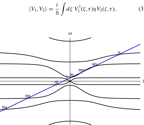
whereωandkare the laboratory frequency and wave number, respectively. The dispersion relation (2) is plotted in Fig.1: there are eight branches, four with positive laboratory fre-quency and four negative-frefre-quency counterparts, symmetric about thek axis. To find orthonormal plane-wave solutions, we define a scalar product on the set of the solutions of our Hamilton-Jacobi equations generalized to complex values,

V1,V2 = i

dζ V1†(ζ,τ)ηV2(ζ,τ), (3)

o

o

o o o

o o

o

nu

no

nl

l lo

mo uo

u

k

whereV is the eight-dimensional vector

V =(A P1P2P3AP1P2P3)T (4)

andηis the selection matrixη=( 0 I4

−I4 0), withI4being the 4×4 identity matrix. This scalar product is a conserved quantity inτ, and therefore the total norm of the quantum states is conserved.

It can also be shown that modes with positive laboratory frequency have positive norm and those with negative fre-quency have negative norm [13,14,25]. In other words, modes belonging to the upper (lower) half plane in Fig.1have positive (negative) norm. In the comoving frame, positive-frequency waves with negative norm appear, which are associated with spontaneous emission from the quantum vacuum. These gener-ated waves have negative laboratory frequency. Negative-norm modes were recently observed in water experiments [7,27] and in optics [22,28]. Due to the conservation of norm, the generation of negative-norm waves signifies a simultaneous increase in positive-norm waves, the generation of correlated waves.

III. MODE CONFIGURATIONS AT A REFRACTIVE-INDEX FRONT

In the previous section we presented a canonical model of light and matter interaction in a dielectric medium. In particular, we highlighted the existence of positive- and negative-frequency modes. We now extend this model to a nonuniform medium.

The simple geometry of a RIF is shown in Fig. 2 in the comoving frame. The medium is composed of two homogeneous regions, separated by the RIF atζ =0, creating a step in the refractive index. The boundary atζ =0 constitutes an infinitely steep RIF which propagates in a steady and rigid way in the positive ζ direction. The right (left) region has dispersion parametersκiR(κiL) andλiR(λiL). Experimentally, this front could be realized by an asymmetric intense pulse of light with a very steep front on one side, similar to a self-steepened soliton pulse [29]. The front is approximately infinitely steep if it is shorter than a wavelength. The step height is the refractive-index change between the regionsδn, defined by

n(ζ)=nLθ(−ζ)+nRθ(ζ)=nR+δn θ(−ζ) (5)

FIG. 2. (Color online) Sketch of the RIF in the moving frame: there are two homogeneous regions of uniform refractive index on the left and right of a dielectric boundary of heightδn. For suitable moving-frame frequencies, light on the left (right) of the RIF may not (may) propagate away to the right as the step moves at superluminal (subluminal) speeds. Light on the left is trapped behind an analog horizon atζ =0.

and illustrated in Fig.2;θ(ζ) is the Heaviside step function. The index change is described by the scaled Sellmeier coefficientsβiL=σβiRandλ2iL=σ λ2iR, where

σ ≈1+2nRδn

n2_R−1 (6)

andnRis the refractive index on the right side [14].

In order to identify the allowed modes of propagation, we consider plane-wave solutions subject to the dispersion relation in both regions for a given comoving frame frequency

ω=γ(ω−uk). This is useful because the frequency ω

is conserved, an expression of energy conservation in the moving frame [13,14,25]. Solutions of fixed ω are found at the intersection points between a line of constant ωwith the various polariton branches in the dispersion diagram (red circles in Fig. 1). Note that we consider only low positive comoving frequenciesω without solutions in the uppermost branch. At any frequencyωthere exists a set of eight discrete (ω,k) solutions to the dispersion relation (2). We either find eight propagating modes or six propagating modes and two exponentially growing and decaying modes, respectively, that take on complexωandk.

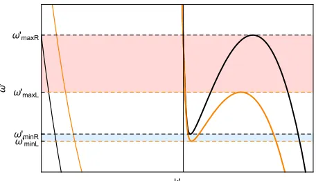
Emission spectra with eight propagating modes on only one side of the boundary were calculated in [14,19]. Here we address the experimentally relevant case allowing for eight modes to propagate on either side of small refractive-index changes. In particular, consider the positive frequency optical branch (where λ2< λ < λ3) in the moving frame, depicted

in Fig. 3. The black (orange) curve is the branch on the right (left) side of the RIF. Again, the number of solutions depends onω. On either side of the RIF there is at least one propagating optical mode for allω. There also is a frequency interval where three propagating modes exist: between the two horizontal dashed black and two dashed orange lines in Fig.3, corresponding to the right and left regions, respectively. Hereafter, these frequency intervals on either side of the RIF

'maxL

'minL

'minR

'maxR

k'

'

are referred to as thesubluminal intervals(SLIs) [ω_minL,ω_maxL] and [ω_minR,ω_maxR].

Inside a SLI, one of the three mode solutions has a positive comoving group velocity ∂ω

∂k. This unique mode allows light on the right of the RIF to escape from it. This middle optical mode (see Fig.1) on the right is calledmoRin what follows. The other two modes have negative comoving group velocity; they move into the boundary from the right. There is a lower (upper) optical mode denotedloR(uoR). On either side we can order the modes by the comoving wave numberkand obtain

k_ωloR /L< kωmoR /L< kωuoR /L(see Fig.3). In the laboratory frame

this translates into ωloR_ω /L < ωωmoR /L< ω

uoR/L

ω (Fig. 1). All three optical-branch modes of the SLI have positivelaboratory group velocity on both sides of the boundary: to an observer in the laboratory frame they propagate in the same direction as the RIF.

Beyond this interval (i.e., ω∈/[ω_min,ω_max]) only one propagating mode remains. Two complex-wave-number roots emerge as pairs of exponentially growing and decaying modes that do not propagate. For ω< ω_min only mode uoR/L remains a propagating mode, whereas for ω> ω_max , only loR/L remains. It can also be seen in Fig. 3 that for all ω

there is one propagating mode that belongs to the negative optical-frequencies branch. This mode has a negative norm and will hereafter be referred to as modenoR/L.

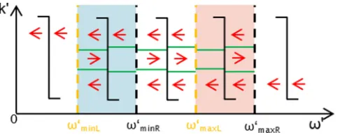
The subluminal frequency interval of the left region is, in general, different from that of the right region. Therefore there exist five different combinations of modes across the RIF, also shown in Fig.4:

(1) ω< ω_minL. One optical propagating mode (uoR/L) exists (real ω and k) on either side of the boundary. All propagating modes exhibit negative group velocities in the moving frame, and therefore no optical horizons exist.

(2) ω_minL< ω< ω_minR. Three propagating modes (loL, moL, anduoL) on the left of the boundary exist, but only one mode (uoR) exists on the right. Only modemoLhas positive group velocity on the left. Light in this mode experiences a white-hole horizon at the RIF as it can approach, but not enter, the right region. To our knowledge, this mode configuration has not yet been described.

(3)ω_minR< ω< ω_maxL. Three propagating modes (loR/L, moR/L, anduoR/L) exist on either side of the boundary. Modes with negative and positive group velocity exist on either side

FIG. 4. (Color online) Diagrammatic explanation of the possible mode configurations for positive-frequency optical modes for various comoving frequencies. Configurations change if two of the modes share their group velocity with the RIF (green lines), which occurs at the frequencies indicated above and in Fig.3.

of the RIF; therefore the RIF is not a one-way door, and no horizon exists for waves of this moving frame frequency.

(4)ω_maxL< ω< ω_{max R}. Only one propagating mode (loL) exists on the left of the boundary, but three modes (loR,moR, and uoR) exist on the right. Only mode moR has positive group velocity on the right side. Light experiences a black-hole horizon at the RIF as it cannot propagate to the right from beyond the RIF. The region on the left (right) of the boundary corresponds to the inner (outer) region of the analog horizon.

(5)ω_{min R}< ω. One propagating mode (loR/L) exists on either side of the boundary. All propagating modes exhibit negative group velocities, and therefore no optical horizons exist.

Note that for very high refractive indices on the left there exists only modeloL, and no subluminal interval in this region, and out of the general case only configurations 1 (with loL instead ofuoL), 4, and 5 remain. In this case, modes within the SLI on the right of the boundary always follow configuration 4. The five configurations introduced here describe a typical experimental combination of horizons with small refractive-index changes.

IV. SCATTERING AT THE RIF

Having derived solutions on either side of the RIF, we now construct “global” solutions, i.e., solutions to the equation of motion that are valid in both regions. These modes correspond to waves scattering at the RIF, and they describe the conversion of an incoming field, even in the quantum vacuum state, to scattered fields in both regions. We follow the approach [14,26,30] to construct these modes and their scattering matrix and then to quantize the solutions to find the photon fluxes due to spontaneous particle creation.

The solutions to the dispersion relation correspond to local modes (LMs) that are defined in either the left or right region. We construct “global modes” (GMs)V as

V= α

LαV_Lαθ(−ζ)+ α

RαV_Rαθ(ζ), (7)

where Lα (Rα) describes the strength of modeαon the left (right) side of the RIF. It can be shown that across the boundary, vector potential, polarization fields, and their derivatives are continuous [14], which constrains half of the coefficients in Eq. (7). We follow the procedure described in [31] and consider GMs whose asymptotic decomposition comprises only a single LM with group velocity towards (in) or away from (out) the RIF. Thus there are as many of these GMs as there are propagating local modes. Half of the GMs emerge from a defining LMαthat moves towards the RIF, forming “global in modes”Vinα_{. The other GMs are “global out modes”V}outα if α is a LM now moving away from the RIF. The sets of

Vin _andVout _{modes are two basis sets of modes because the}

LMs are the complete physical (i.e., nondivergent) solutions in the asymptotic regions. Hence the scattering matrixSis the transformation of modes from the out basis to the in basis:

Vin,α₌ β

Scattering and spontaneous photon creation occur as the input state vacuum does not correspond to the vacuum state in the out basis; that is, the spontaneous emission follows fromS.

We postulate the equivalent of the standard equal-time commutation relations onAandPiand thus quantize the local field modes and their momenta:

[A(ζ),A(ζ)]=iδ(ζ −ζ), (9)

[Pi(ζ),Pj(ζ

_)]=iδ

ijδ(ζ −ζ). (10) We expand the real field V [Eq. (4)] on the basis of local frequency eigenmodes

V = dω

α

V_ωαaˆαω+V α ω∗aˆ

α_† ω

(11)

that are properly normalized with respect to the scalar product (3) under the condition

Vα1 ω₁,V

α2

ω₂=δ(ω2 −ω1)δα2α1. (12)

The operators ˆaα_ω and ˆaαω† are the annihilation and creation operators of the field modeα. Alternatively, we can expand the field over only positive frequencies, including negative-norm modes in the expansion:

V =

∞

0

dω

α∈P

V_ωαaˆωα+

α∈N

V_ωαaˆωα†

+H.c., (13)

where P(N) is the mode set of positive (negative) norms. Writing the global field V in the basis of global in modes induces quantization onto the GMs:

V= ∞

0

dω

α∈P

Vin,α ω aˆ

in,α ω +

α∈N

Vin,α ω aˆ

in,α_† ω

+H.c.,

(14)

and a similar expression can be written for V using the global out modes. The expansion (14) for in and out modes defines the annihilation and creation operators for the global modes as well as the transformation between in and out creation and annihilation operators. If ˆAin _{is a row vector}

containing all the annihilation and creation operators for positive- and negative-norm global in modes, respectively, and

ˆ

Aout_{is the corresponding variable for the out modes, then the}

transformation of operators is [14] ˆ

Aout =AˆinS. (15)

Using Eq. (15), we obtain the flux density of photons Iα in mode α, the number of particles per unit time τ and bandwidth in the moving frame, as [14]

Iα =2π0|aˆ

α_† ωaˆ

α ω|0

τ . (16)

In terms of the scattering matrix, the flux density in modeα

follows from Eqs. (15) and (16):

Iα=

¯

α

|Sαα¯ |2, (17)

where ¯αis a mode with a norm opposite in sign toα. Spectra for positive-norm modes and for single SLIs were calculated

0.03 0.06 0.09 0.12 10−6

10−4 10−2 1

'

minR 'maxL 'maxR

'(eV)

Flux

density

I'

'

moR

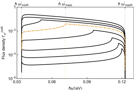
FIG. 5. (Color online) Spectrum of emission into the uniquely right propagating modemoRon the right side of the RIF. Emission is calculated in the moving frame of velocityu=0.66c. The number of particles per time and bandwidth, the flux density, is displayed for increasing values ofδn(1×10−3_{, 2×10}−3_{, 4×10}−3_{, 1×10}−2_{, 2×10}−2 (orange dot-dashed line), 3×10−2_{, 4×10}−2_{, 5.6×10}−2_{). The spectrum} is confined to a finite interval over which the modemoRexists.

with this relation in [14,19]. We now move on to obtain the spectra of emission for any frequency in all modes, for all mode configurations (see Sec.III), and for a variety of refractive-index changesδn.

V. EMISSION SPECTRA AND PHOTON FLUX We proceed to use the S matrix to compute the spectra of emission into all optical modes as seen from the moving and laboratory frames. We consider modes in bulk fused silica. The material resonances are λ₁,2,3=9904, 116, and

68.5 nm, respectively, and the elastic constants are κ₁,2,3=

0.07142,0.03246, and 0.05540, respectively. The velocity of the RIF isu=0.66c, corresponding to a group index of 1.5.

We first consider spectra in the moving frame. Figure 5

displays the spectrum of emission into moR, the unique right-going mode (black-hole emission), for different index changes δn. Spectral emission is constrained to the right

0.03 0.06 0.09 0.12 10−4

10−3 10−2 10−1

'(eV)

Flux

density

I''

moR

0.03 0.06 0.09 0.12 10−4

10−3 10−2 10−1

'

minR 'maxR

'

minL 'maxL

'(eV)

Flux

density

I''

FIG. 7. (Color online) Emission spectra of each optical mode in the comoving frame (u=0.66c, δn=0.02): emission into mode noL, purple solid line;loL, blue dashed line;uoL, green dotted line; moR, orange dot-dashed line.

SLI [ω_minR,ω_maxR], where the mode moR exists. An optical horizon, however, exists for only part of this interval, i.e., [ω_{max L},ω_maxR], because at lower frequencies the SLIs of the left and right overlap (see Fig. 3). As can be clearly seen, the absence of a horizon leads to a significant decrease in the emission, i.e., mode coupling, although some emission remains. In the case of a large index change (e.g.,δn=0.056), as calculated and observed in [14], the spectral shape is not thermal as expected from a finite subluminal interval. Here we observe a remarkable feature: the shape of the spectrum above ω_{max L}, where a horizon exists, is independent of the index change. This can be more clearly seen in Fig. 6, in which the spectra for smaller index changes are scaled up to compensate the lower single-frequency rate. All traces over orders of magnitude of index changes line up to the same shape, making it a universal signature of analog black-hole emission. Note also that the shape differs for emission outside the SLI.

Next, we consider spectra of emission into each mode (i.e., noL,loL,uoL,moR) for fixedδn=0.02, as displayed in Fig.7. The strongest emission occurs into the optical mode with

negative norm,noL. This emission is due to coupling with all the other positive-norm modes in the medium and is strongest where this superluminal mode couples to a subluminal mode (ω_maxL< ω< ω_maxR).

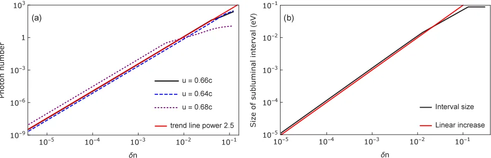
It is interesting to calculate the total photon flux over the SLI [ω_minR,ω_{max R}] by integrating over the spectrum of Fig. 5. In order to convert the flux to a realistic, although very approximate, photon number, we assume that the RIF propagates over a distance of 1 mm. The resulting photon number as a function of index changeδnis given in Fig.8(a). The number of photons excited from the vacuum first grows with power≈2.5 ofδnuntilδn=0.052. The emission spectrum becomes wider in a linear way, as shown in Fig.8(b). Thus the emission rate for a single mode increases withδn3/2. This result is surprising and will be further investigated elsewhere. For a very high induced index change, i.e., for

δn0.052, the spectral width saturates, and the emission rate grows slower accordingly. These index steps are difficult to reach experimentally by nonlinear optical pulses, however.

The spectra calculated above would be observable in the moving frame. In an actual experiment the detectors are located in the laboratory frame, and thus the spectrum observed is different. For each mode, the rate of photon production per unit time and unit frequencyωin the laboratory frame is derived from the moving frame rate as [14]

Iα=

1− u

vg(ω)

Iα, (18)

wherevg(ω) is the laboratory group velocity atω. The spectral density as a function of frequency converts to wavelength by the factor ω2_{/(2π c). A laboratory spectrum for a single}

mode was calculated in [14]. However, this spectrum is not observable for the following reason: on either side of the RIF, each moving frame frequency ω corresponds to up to eight different laboratory frequencies depending on the mode involved, as in Fig.1. Note that we calculate the emission with only positive laboratory group velocity. Thus each mode has a unique direction of group velocity in both frames independent of the side of the RIF. Hence, of the modes left and right of the RIF, half define global out (emission) modes. Conversely, the emission at a fixed laboratory frequency may arise from

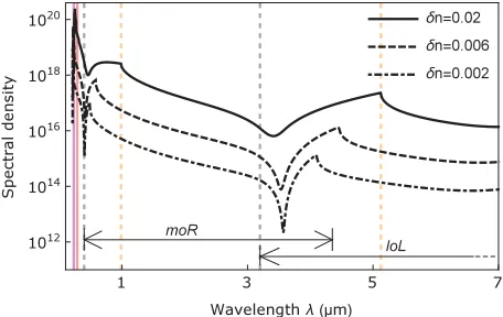
FIG. 9. (Color online) Emission spectral density in the laboratory frame. At each wavelength the total spectral flux density, the number of photons emitted per unit time and unit bandwidth, is the sum of contributions from all modes. Emission is concentrated in the UV in a narrow spectral peak generated from modenoR. Outside the peak the emission decreases except for spectral intervals corresponding to black- and white-hole analog horizons. Spectra are calculated for wavelengths above the violet line, beyond which there are no contributions from the uppermost dispersion branch. The red line corresponds to ω=0 (phase velocity horizon). The black and orange dashed lines indicate the interval of the black-hole (white-hole) mode configuration for the moR(loL) mode at short (long) wavelengths.

several optical modes. We proceed to calculate for successive frequenciesωthe emission rates in each associated global out mode, obtaining a laboratory frame spectrum for each mode. We then add up the spectra to obtain the total spectral emission. Starting atωm, the lowest positive optical frequency, we obtain emission into outgoing mode loLon the left, then moR on the right, followed byuoLon the left and, finally,noLon the left.

Figure9shows laboratory spectra for three index changes. As the spectrum is composed of contributions from different modes for different mode configurations, it exhibits a number of sharp features. The largest spectral density is obtained around 250 nm and corresponds to emission from the negative-norm mode noL. Emission is generated by the pairwise coupling of two modes of opposite norm. Hence modenoLis the only negative-norm mode on the optical branch and covers a rather small laboratory spectral interval between the solid violet and red vertical lines in Fig.9. Therefore, all emission due to the coupling of two optical modes leaves a contribution within this emission peak in the UV spectral range. The coupled positive-norm mode (i.e., the partner photon), if optical, can be found at the remaining optical frequencies. We choose to limit the range of optical wavelengths such that no modes in the uppermost branch are excited, resulting in a cutoff at 230 nm. Not all coupled mode pairs are separated by a black- or white-hole-type horizon. For example, intervals with horizons, as schematically sketched in Fig.4, are found between the two sets of black and orange dashed lines in Fig.9but not in the adjacent spectral regions. The short (long) wavelength interval corresponds to a black-hole (white-hole) configuration. The presence of optical horizons leads to an enhancement of the emission on the background of the

horizonless emission that seems to decay from the ultraviolet to the infrared. Modes moR and loL exhibit clear horizon emission profiles between the black and orange dashed lines, and their intervals of emission are indicated by arrows. Over the visible range, the emission frommoRdominates. Figure9

also shows traces for lower nonlinearities. As expected, the spectral density decreases, and the intervals of optical horizons, associated with strong emission, become smaller. The red line at∼290 nm corresponds to zero moving-frame frequencyω; no major spectral features seem to be associated with this position.

The quantum state at the output is expected to be a two-mode squeezed vacuum state if only two two-modes were involved. However, for each moving-frame frequency, each mode can couple to up to five positive-norm and three negative-norm modes. Thus, we expect the final quantum state on the optical branch to be in a partly mixed state across the optical modes. Yet coupling between particular mode pairs seems to dominate in parts of the spectrum, in particular within the optical branch. Further characterization of the exact state emerging is needed.

VI. CONCLUSION

Emission of light from the quantum vacuum has recently attracted attention [13,14,19,32] due to the high emission rates expected in the presence of an analog horizon and the hope to observe analog Hawking radiation. Using a fully analytical model introduced in [14], the spontaneous emission of light from a moving dielectric boundary, a refractive-index front, can be calculated. The model can be used to study any dispersive medium phenomenologically described by Sellmeier equations.

In this work we have focused on the case of SLIs on both sides of the RIF. We calculate the emission for a system based on bulk fused silica. Our approach is interesting because we can show how the emission is structured into intervals with black-hole, white-hole, and no horizons and how these horizons lead to an increase in the spectral density in the laboratory over a general decay. To our understanding, the enhancement of emission due to horizons is a common feature of realistic refractive-index changes. For index changes beyond the damage threshold no enhancement was observed [19]. Additionally, because we consider contributions from all modes, we have found that the emission is dominated and characterized by a peak in the (laboratory) UV that corresponds to photons emitted in the negative-norm mode. We show that the emission spectrum from the analog black hole has a unique shape, which is independent of the index change. It is not the thermal shape that is expected from a nondispersive analog black-hole horizon. We also calculate the emitted flux, and as a result, the flux increases as a power law of exponent 2.5 for smaller index steps, as more and more frequency modes appear to participate in the emission at the analog black-hole horizon. Whereas previous calculations have mainly focused on the Hawking-like emission in the moving frame, these results reveal signatures of the quantum vacuum emission important for the experimental observation, such as the nonlinear scaling, spectral shape, and mode configuration.

emission into other modes. This analysis would allow for a better prediction of the exact quantum state produced, a key connection to the Hawking effect. The analysis can also be extended to more general variations of the refractive index as well as broader choices of media, such as waveguides.

ACKNOWLEDGMENTS

The authors would like to acknowledge useful discussions with S. Finazzi and R. Parentani, as well as support from EPSRC via Grant No. EP/L505079/1.

[1] S. Hawking,Nature (London)248,30(1974). [2] S. Hawking,Commun. Math. Phys.43,199(1975). [3] W. G. Unruh,Phys. Rev. Lett.46,1351(1981).

[4] C. Barcelo, S. Liberati, and M. Visser,Living Rev. Relativ.8,

12(2005).

[5] C. Barcelo, S. Liberati, and M. Visser,Living Rev. Relativ.14,

3(2011).

[6] S. J. Robertson,J. Phys. B45,163001(2012).

[7] S. Weinfurtner, E. W. Tedford, M. C. J. Penrice, W. G. Unruh, and G. A. Lawrence,Phys. Rev. Lett.106,021302(2011). [8] L. J. Garay, J. R. Anglin, J. I. Cirac, and P. Zoller,Phys. Rev.

Lett.85,4643(2000).

[9] L. J. Garay, J. R. Anglin, J. I. Cirac, and P. Zoller,Phys. Rev. A

63,023611(2001).

[10] P. D. Nation, J. R. Johansson, M. P. Blencowe, and F. Nori,

Rev. Mod. Phys.84,1(2012).

[11] G. E. Volovik, The Universe in a Helium Droplet, 2nd ed., International Series of Monographs on Physics Vol. 117 (Oxford University Press, Oxford, 2009).

[12] H. S. Nguyen, D. Gerace, I. Carusotto, D. Sanvitto, E. Galopin, A. Lemaitre, I. Sagnes, J. Bloch, and A. Amo,Phys. Rev. Lett.

114,036402(2015).

[13] T. Philbin, C. Kuklewicz, S. Robertson, S. Hill, F. Koenig, and U. Leonhardt,Science319,1367(2008).

[14] S. Finazzi and I. Carusotto,Phys. Rev. A87,023803(2013). [15] S. Robertson, Ph.D. thesis, University of St Andrews (2011). [16] U. Leonhardt and T. G. Philbin, inProgress in Optics(Elsevier,

Amsterdam, 2009), pp. 69–152.

[17] F. Belgiorno, S. L. Cacciatori, M. Clerici, V. Gorini, G. Ortenzi, L. Rizzi, E. Rubino, V. G. Sala, and D. Faccio,Phys. Rev. Lett.

105,203901(2010).

[18] S. Finazzi and I. Carusotto,Eur. Phys. J. Plus127,78(2012). [19] S. Finazzi and I. Carusotto, Phys. Rev. A 89, 053807

(2014).

[20] A. Choudhary and F. K¨onig,Opt. Express20,5538(2012). [21] M. Petev, N. Westerberg, D. Moss, E. Rubino, C. Rimoldi, S.

L. Cacciatori, F. Belgiorno, and D. Faccio,Phys. Rev. Lett.111,

043902(2013).

[22] J. McLenaghan and F. K¨onig,New J. Phys.16,063017(2014). [23] S. Robertson and U. Leonhardt,Phys. Rev. E90,053302(2014). [24] S. Robertson,Phys. Rev. E90,053303(2014).

[25] F. Belgiorno, S. L. Cacciatori, and F. Dalla Piazza,Phys. Rev. D

91,124063(2015).

[26] J. J. Hopfield,Phys. Rev.112,1555(1958).

[27] G. Rousseaux, C. Mathis, P. Ma¨ıssa, T. G. Philbin, and U. Leonhardt,New J. Phys.10,053015(2008).

[28] E. Rubino, J. McLenaghan, S. C. Kehr, F. Belgiorno, D. Townsend, S. Rohr, C. E. Kuklewicz, U. Leonhardt, F. K¨onig, and D. Faccio,Phys. Rev. Lett.108,253901(2012).

[29] G. P. Agrawal, inNonlinear Fiber Optics, 4th ed., edited by G. P. Agrawal, Optics and Photonics (Academic Press, San Diego, 2006).

[30] B. Huttner and S. M. Barnett,Europhys. Lett.18,487(1992). [31] J. Macher and R. Parentani,Phys. Rev. D79,124008(2009). [32] F. Belgiorno, S. Cacciatori, and F. Piazza,Eur. Phys. J. D68,