The information content of a limit order book : the case of an FX market

(1)

University of Warwick institutional repository: http://go.warwick.ac.uk/wrap

This paper is made available online in accordance with publisher policies. Please scroll down to view the document itself. Please refer to the repository record for this item and our policy information available from the repository home page for further information.

To see the final version of this paper please visit the publisher’s website. Access to the published version may require a subscription.

Author(s): Roman Kozhan and Mark Salmon

Article Title: The information content of a limit order book: The case of an FX market

Year of publication: 2011 Link to published article:

http://dx.doi.org/10.1016/j.finmar.2011.07.002

Publisher statement: “NOTICE: this is the author’s version of a work that was accepted for publication in Journal of Financial Markets. Changes resulting from the publishing process, such as peer review, editing, corrections, structural formatting, and other quality control mechanisms may not be reflected in this document. Changes may have been made to this work since it was submitted for publication. A definitive version was subsequently published in Journal of Financial Markets, VOL: 15, ISSUE: 1, February 2012, DOI:

(2)

The information content of a limit order book: the case

of an FX market

I

Roman Kozhana,∗, Mark Salmonb

a_{Warwick Business School, University of Warwick, Scarman Road, Coventry, CV4 7AL,} UK; e-mail: Roman.Kozhan@wbs.ac.uk

b_{Warwick Business School, University of Warwick, Scarman Road, Coventry, CV4 7AL,} UK; e-mail: Mark.Salmon@wbs.ac.uk

Abstract

In this paper we examine the question of whether knowledge of the information contained in a limit order book helps to provide economic value in a simple trading scheme. Using Dollar Sterling tick data, we find that despite the in-sample sta-tistical significance of variables describing the structure of the limit order book in explaining tick-by-tick returns, they do not consistently add significant economic value out-of-sample. We show this using a simple linear model to determine trad-ing activity, as well as a model-free genetic algorithm based on price, order flow, and order book information. We also find that the profitability of all trading rules based on genetic algorithms dropped substantially in 2008 compared to 2003 data.

JEL classification: D81, F31, C53

Keywords: profitability,limit order book, high-frequency data, algorithmic trading

I_{We are grateful to an anonymous referee and Bruce Lehmann (the editor), whose}

in-sightful comments greatly improved the paper. We also thank Martin Evans, Matthijs Fleischer, Thierry Foucault, Lawrence Harris, Rich Lyons, Chris Neely, Carol Osler, Richard Payne, Dagfinn Rime, Lucio Sarno, Nick Webber and Paul Weller for their helpful comments and suggestions. We remain responsible for all errors.

(3)

1. Introduction

One important issue in recent market microstructure research has been whether knowledge of the structure of the limit order book is informative regarding future price movements. There is a growing body of theoretical work suggesting that limit orders imply the predictability of short term asset returns (see Handa and Schwartz, 1996, 2003; Harris, 1998; Parlour, 1998; Foucault, 1999; Rosu, 2010 among others). This is in contrast with earlier papers that implied that informed traders would only use market orders (see Glosten, 1994; Rock, 1996; Seppi, 1997). This debate has also been carried out empirically by Harris and Hasbrouck (1996), Kavajecz (1999), Harris and Panchapagesan (2005), Cao, Hansch and Wang (2009), and Hellstr¨om and Simonsen (2009), all of whom demonstrated that asset returns can be explained by limit order book information, such as depth and order flow. However, these studies have failed to demonstrate that the predictability of returns can be exploited in economic terms. In this paper we go beyond statistical significance and consider the economic value of limit order book information in an FX market.

We address this question by explicitly constructing trading strategies based on full limit order book and price information in the FX market. These strategies only use historical information in order to ensure that trading can be implemented in “real time” and focus on the economic value of ex-ante predictability in out-of-sample prediction exercises.

(4)

a model-free way by employing a genetic algorithm. Genetic algorithms serve as a systematic search mechanism for the best trading rule from amongst a huge universe of potential rules given the particular information set and have been successfully applied in a number of financial applications, most notably by Dworman, Kimbrough and Laing (1996), Chen and Yeh (1997a), Chen and Yeh (1997b), Neely, Weller and Dittmar (1997), Allen and Karjalainen (1999), Neely and Weller (2001), Dempster and Jones (2001), Chen, Duffy and Yeh (1999), Arifovic (1996). Rather than adopting a single specific forecasting model, the genetic algorithm searches from a very large set for that trading rule which exploits the information most profitably. We then test if this approach generates significantly higher returns when new information constructed from the limit order book is included alongside price information. It is important to recognize the theoretical and practical coherence offered by using genetic algorithms. A number of authors, since Leitch and Tanner (1991), have argued that the use of purely statistical criteria to evaluate forecasts and trading strategies is inappropriate (e.g., Satchell and Timmer-mann, 1995; Granger and Pesaran, 2000; Pesaran and Skouras, 2002, and Granger and Machina, 2006). The issue turns on the appropriate loss func-tion and whereas many statistical evaluafunc-tion criteria are based on a quadratic loss, practical criteria are more likely to be based on the utility derived from profits. Critically, from our point of view, the genetic algorithm constructs trading rules using the same loss function as is used to evaluate the out-of-sample performance of the trading strategy, unlike a linear regression model where a statistical quadratic loss is used in estimation.

(5)

profitability of trading strategies in “real time” is transaction costs.1 _We

analyze the performance of our trading rules on the basis of the best bid and ask prices using tick-by-tick data and so explicitly take into account transaction costs as measured by the bid-ask spread. This allows us to test if predictable components in exchange rate returns are economically exploitable net of transaction costs.

Using data on the U.S. dollar sterling exchange rate for five separate weeks2 we find statistical predictability in the exchange rate and profitability net of transaction costs for samples drawn from 2003. However, we find that the profitability in more recent data from 2008 decreases substantially and in most cases is not significantly different from zero. This could be explained by the tremendous recent growth in high-frequency algorithmic trading within financial markets.

We also find in-sample statistical significance of limit order book informa-tion in all sample periods. Specifically, we show that both static informainforma-tion about liquidity beyond the best prices and order flow of both market and limit orders have some ability to explain future short-term movements of the exchange rate. However, we find little or no value in an economic sense in al-lowing the predictor to exploit information in the order book beyond of that contained in the best prices. In other words, we fail to significantly increase out-of-sample returns from our trading strategy when we use liquidity and order flow information. Our main finding then is that any information

con-1_{Neely and Weller (2003) for instance emphasize the critical role of transaction costs}

and inconsistences between the data used by practitioners and in academic simulations.

2_{We have examined data from a number of different periods and find similar results for}

(6)

tained in limit orders beyond best prices is not robust enough to be exploited profitably out-of-sample, particularly in the most recent 2008 data.

The remainder of the paper is organized as follows. In Section 2 we provide a literature review relevant to this research. Section 3 contains a description of the data used in the study and the methodology employed in the analysis. The main results are given in Section 4 and Section 5 concludes.

2. Literature review

Limit-order book markets potentially offer greater transparency when compared with quote-driven markets. Whereas dealer markets will usually only release the dealers’ best quotes, a limit-order-book can allow its users to view the depth at a number of price levels away from the market price. The NYSE, under the OpenBook program, publishes aggregate depths at all price levels on either side of the book and under LiquidyQuote displays a bid and offer quote, potentially different from the best quotes in the market. NAS-DAQ’s SuperMontage order entry and execution system displays aggregate depths at five best price levels on either side and employs a scan function that allows traders to assess liquidity further along the book. The question is how this incremental information on the structure of a limit order book is used and whether it adds economic value in the process of price discovery.

(7)

(8)

information than market orders. When this is the case and the number of traders who can discover the private information is small, then using mar-ket orders will reveal too much information implying higher trading costs. Bloomfield, O’Hara and Saar (2005), in a laboratory experiment, find that informed traders submit more limit orders than market orders. They exploit their informational advantage early in the trading period to find mispriced limit orders moving the market towards the true price, thereby progressively reducing the value of their information. As the end of the trading period approaches, they switch increasingly to limit orders, as the value of their informational advantage falls away.

(9)

infor-mation content of the limit order book to explain returns using variogram techniques, which involves no specific parametric model. They show clear in-sample ability to explain very short run movements in the USD/DM rate using a range of measures of order book structure. Hellstr¨om and Simonsen (2009), using a count data time series approach, find that there is informa-tional value in the first levels of the bid- and ask-side of the order book. They also show that both the change and the imbalance of the order book statistically significantly explain future price changes. Offered quantities at the best bid and ask prices on data from the Swedish Stock Exchange reveal more information about future short run returns than measures capturing the quantities at prices below and above. The impacts are most apparent at the one minute aggregation level, while results for higher aggregation levels generally show insignificant results. These results would suggest that the informational content of the order book is very short-term.

While the above mentioned papers focus on in-sample statistical signif-icance, there are also several papers demonstrating some ability of condi-tioning information to predict future movements of returns out-of-sample.3

Huang and Stoll (1994) found that differences in quoted depth predict fu-ture returns at five-minute intervals out-of-sample. Evans and Lyons (2005, 2006) were among first to document the forecasting power of customer order

3_{This distinction is important both theoretically and empirically. It is widely recognized}

(10)

flow to outperform a random walk benchmark. Froot and Ramadorai (2005) report that order flow contains some information for future exchange rate returns in low frequency data. Rime, Sarno and Sojli (2010) employ data for three major exchange rates from the Reuters electronic interdealer trad-ing platform and confirm these findtrad-ings. In contrast to the above studies, Danielsson, Luo and Payne (2002) find limited and Sager and Taylor (2008) find no evidence of superior forecasting ability of order flow over random walk models at different forecast horizons.

There are not many papers falling into the second group that focus on whether or not the market information can be exploited economically by market participants. Chordia and Subrahmanyam (2004) find profitability of future stock returns using order imbalance; Della Corte, Sarno and Tsiakas (2009) and Rime, Sarno and Sojli (2010) find profitability of exchange rate returns using transaction order flow but only in the long run. However, neither of these papers consider limit order book information in their trading strategies. A notable exception is a paper by Latza and Payne (2010), who considered the forecasting power of market and limit order flows on stock returns and show that both can forecast returns. They show, via simulation, that dealers who time the execution of the trades on the limit order flow can reduce the cost of trading customer orders by up to 20%.

3. Data and methodology

(11)

make sure that our results are not driven by the use of any particular sam-ple period, we use five different data sets: weeks commencing on January 13, 2003, February 10, 2003, March 17, 2003, and two days on March 31 and April 1, 2008 (there is a much higher frequency of trades in 2008, as we discuss below). The data we analyze consists of continuously recorded limit and market orders and their volumes between 07:00-17:00 GMT which allows us to reconstruct the full limit order book on a tick-by-tick basis. For each entry, the data set contains a unique order identifier, quoted price, order quantity, quantity traded, order type, transaction identifier of order entered or removed, status of market order, entry type of orders, removal reason, and date and time of orders entered and removed. The data time stamp’s preci-sion is 1/100th of a second and the minimum trade size in Reuters electronic trading system is 1 million pounds sterling.

3.1. Summary statistics

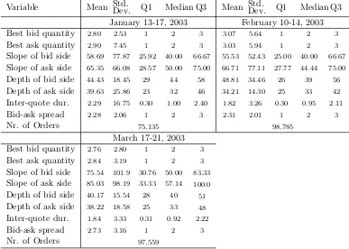
Table 1 reports the summary statistics for transaction and limit order data for the different sample periods. Average inter-quote durations (speed of limit order arrival or removal) are 2.29, 1.82, and 1.84 seconds for first three samples and 0.1 and 0.09 seconds for the two 2008 samples. This demon-strates that the electronic market is very active and critically its activity has grown tremendously from 2003 to 2008. There are 75,135, 98,785, and 97,559 orders for the three weeks in 2003 and 594,519 and 388,259 on March 31 and April 1, 2008, respectively. The average values of the bid-ask spread from our samples are 2.28, 2.21, and 2.73 basis points in 2003 and 2.53 and 2.59 basis points in 2008, indicating that D3000 is a very tight market.

(12)

2003 and 2008 samples, there is a huge jump in market liquidity as measured by the slope of the limit order book and its depth. The average slopes of the limit order book in the 2003 subsamples are 58.69, 55.53, and 75.54 basis points per billion of currency trade for the bid side and 65.35, 66.71, and 85.03 for the ask side.4 _{In the 2008 samples, the slope values were 20.89 and}

19.52 for bid side and 21.52 and 20.26 for ask side, indicating that the limit order book became about three times flatter in 2008 than it was in 2003. Also, the depth of the market almost doubled. These summary statistics indicate that the currency pair we are studying is traded in a highly liquid market.

Insert Table 1 about here

3.2. Hypotheses

We are interested in two main hypotheses. The first is whether the ex-change rate is predictable in terms of statistically significant economic value (economic predictability). Thus,

Hypothesis 1. The exchange rate returns is not economically pre-dictable at high frequency.

The second question is whether limit order book information adds eco-nomic value over that provided by the basic price information available.

Hypothesis 2. Limit order book information does not add significant economic value to the predictability of the exchange rate at high-frequency.

4_{We construct the slope of the demand and supply curves in our limit order book using}

(13)

As mentioned above, we build trading strategies that are designed to exploit any profitable pattern in the exchange rate and test the profits ob-tained for significance. By varying the information set used in these trading rules, we are able to differentiate the predictive power of limit order book information from that contained in past prices and volumes.

As the majority of existing research has focused on linear predictive mod-els, we also employ alinear modelto forecast future exchange rate movements as a benchmark. Apart from this linear model we also use agenetic algorithm as a general non-parametric device to construct trading rules. This approach has the advantage that it is model free and designed to exploit both linear and any non-linear dependency between future returns and predictors. The specification of the genetic algorithm trading rules evolve according to their “fitness”, which is determined by an economic profit based criterion. This approach is not therefore susceptible to the criticism that any result we find would have been due to the assumption of a specific trading rule we had selected ex ante.

Since we want to keep our trading strategies implementable in “real time”, we need to ensure that they are based exclusively on historical data available at the time of trade. We use an in-sample period to construct the rules and then check their performance out-of-sample. We describe the implementation of our approach next.

3.3. The information sets

(14)

generating the trading signal.

1. Screen information (denoted by Screen hereafter) contains best limit order prices (both bid and ask) and their quantities as time series, the bid-ask spread, the level of mid-quotes, and the inter-quote dura-tion. This information is considered as the basic set, which is normally available to all traders. It is also contained as a subset in the three information sets defined below.

2. Limit order book information(denoted by Book hereafter); in addition to the variables mentioned above, includes total depth, the number of layers in the limit order book, the difference between the best and the second best price (both, bid and ask), the slopes of the bid and ask curves of the limit order book, time series of the levels of quantity weighted quotes, and the quantity weighted mid-quote, the quantity weighted bid-ask spread, and the difference between the mid-quote and the quantity weighted mid-quote. By depth we mean the total quantity available at the moment in the limit order book on the particular side of the book (demand or supply). The slope of the bid side of the limit order book is defined as,

slopebid = pbid₁ −pbid₂ /q₁bid,

where pbid

1 and pbid2 are the best and the second best prices on the bid

side respectively andqbid

1 is the quantity available at the best bid price.

The slope of the ask schedule is defined analogously. The quantity weighted bid price is defined as,

wpbid = X i

pbid_i ×qbid_i

!

/X i

(15)

where the index i runs through all available levels of bid quotes. The quantity weighted mid-quote is,

wmid= wpbid+wpask/2

and the quantity weighted bid-ask spread is,

wspread=wpask−wpbid.

3. Order flow information(denoted byOrder hereafter) contains the screen information set plus order flow information. Following Latza and Payne (2010), we use two different types of order flow: limit order flow and transaction order flow. Limit order flow is further decomposed into or-der flow on the best prices (the inside oror-der flow) and oror-der flow outside the best prices (the outside order flow). We construct 1 and 20 minute as well as 1 tick order flow variables for each side of the limit order book. By 1 tick order flow we mean the volume of the most recent order of the corresponding type (either market order, limit order at the best price or the limit order outside the best price) strictly preceding the time of decision making.

4. Full information (denoted by Full hereafter) combines all three types of conditioning information mentioned above.

(16)

we will detect it in our experiments. If we cannot find added value, then it would imply that limit orders placed outside the best prices do not carry any significant information about future returns.

3.4. The trading mechanism and fitness function

We measure the fitness of trading rules by means of the cumulative returns from the following simple trading strategy. The trader buys or sells short 1 million pounds sterling according to the signal provided by the selected trad-ing rule. This allows us to control for the potential price impact of trade since we can ensure that the liquidity necessary to complete a transaction with the minimum trade size is present in the market.5 _{As new information arrives}

from the market, the trader re-evaluates the trading signal and updates his position accordingly. This means that as soon as the trader observes any change in the limit order book, he can change or keep the same position depending on the outcome of the signal.

Under such a trading scheme, the trader is potentially able to trade at every single instant. In order to control for trading frequency, we add a trading threshold to the strategy. According to this, the trader is allowed to trade only if the exchange rate exceeds a band of ±k, relative to his last transaction price. More formally, let zt denote the state of the investor’s position at time t. That is, zt = 1 corresponds to a long position in sterling and zt =−1 corresponds to a short position. The trader will re-evaluate his position only if |pt−pt1| ≥k, where pt is price at time t and t1 denotes time

of the trader’s last transaction.

5_{We assume that traders can execute transactions at the current price immediately and}

(17)

The coefficientk serves as an inertia parameter to filter out weak trading signals. The idea of such “filter rules” goes back to Alexander (1961) and Fama and Blume (1966). The parameterkdetermines an “inertia band” that prompts one to trade only once a realization of the exchange rate exceeds the value of a certain characteristic (past realized values of the exchange rate in our case) by a value of k. A larger inertia band (larger k) filters out more trades, thus reducing trading frequency. The use of an inertia parameter also has a behavioural interpretation based on the notion of ambiguity aversion. For instance, Easley and O’Hara (2010) show that in the face of Knight-ian uncertainty incomplete preferences may lead to an absence of trading. Traders will revise their position only if the trading signal is confirmed by other criteria that they have at their disposal, which is very often provided by simple technical tools.

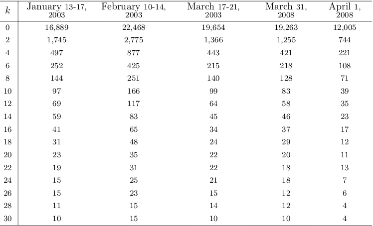
Table 2 presents how many times the trader re-evaluates the position during the out-of-sample period for different values of k. A zero value of k means that trades can take place every time the mid-quote of the exchange rate changes and hence exhibits the largest number of transactions. As k increases, the trading frequency drops. Fork= 30, only up to 10 transactions per day can be made.

We use simple cumulative returns as a performance measure to evaluate the profitability of trading strategies:

Rc= Y

t

(18)

where rt = pt −pt−1

pt−1 is the one-period return of the exchange rate. Here pt denotes the corresponding best bid pbid_t or best ask pask_t price.

3.5. The linear trading rule

The linear model’s predictions are generated using a linear regression. We use an in-sample period to estimate the regression model where the dependent variable is the one step ahead mid-quote exchange rate return rt+1 and the

regressors are timetdated values of all the variables contained in the relevant information set. Out-of-sample forecasts of future exchange rate returns serve as signals for a simple binary trading rule, i.e., positive (negative) predicted values of future returns are associated with a “buy” (“sell”) signal. Based on these signals, we construct a trading strategy as described above and evaluate its out-of-sample performance for different values of the inertia parameterk.

3.6. Genetic algorithm trading rule

The genetic algorithm provides an effective method for searching over space of potential trading rules, both linear and non-linear. This method allows us to evaluate predictability as generally as possible and not impose any effective restriction on the form of the model, predictor or trading rule. The genetic algorithm is a computer-based optimization procedure that uses the evolutionary principle – the survival of the fittest – to find an optimum. It provides a systematic search process directed by performance rather than gradient.6

6_{Nix and Vose (1992) and Vose (1993) use a Markov Chain framework to show that}

(19)

popula-Starting from an initial set of rules, the genetic algorithm evaluates the fitness of various candidate solutions (trading rules) using the given objective function. It provides as an output, solutions that have higher in-sample cumulative returns on average.

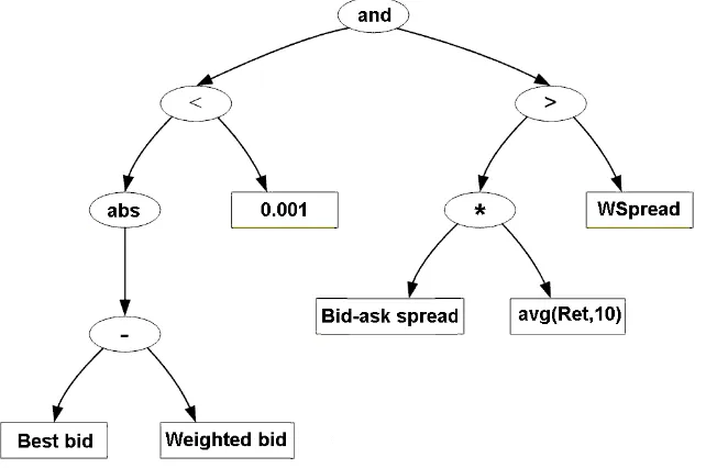
We build a trading rule as a binary logical tree, which produces true or false signals given the set of input variables. If the value of the rule is “true,” it gives the signal to “buy” an asset. If the rule is “false,” –the trader “sells” the asset short. The rules are represented in the form of randomly created binary trees with terminals and operations in their nodes. We employ the following choices of operations and terminals.

Operations: The function set used to define the technical rules con-sists of the binary algebraic operations {+,−,∗, /,max,min}, binary order relations {<, >,≤,≥,=}, logical operations {and,or}, and unary functions

{abs,−}of absolute value and change of sign.

Terminals: The terminal set contains the variables, which take their values from data and are updated every time new information arrives in the market. Thus, it allows the conditioning information sets to update the trading rule as time passes. The genetic algorithm also explicitly computes lag values of the conditioning variables, their moving average values, and maxima and minima over different periods. The terminal set also includes real numbers as terminal constants.

An example of a tree and the corresponding trading strategy is given

(20)

in Figure 1. It presents a trading rule that generates a signal “buy” if the current quantity weighted spread is less than the last ten trades average returns times the bid-ask spread and the absolute value of the difference between the quantity-weighted bid and best bid price is less then 0.001. Otherwise, the signal is “sell.”

Insert Figure 1 about here

Two operations of crossover and mutation are applied to create a new generation of decision rules based on the genetic information of the fittest candidate solutions.

Crossover: For the crossover operation, one randomly selects two parents from the population based on their fitness. A node within each par-ent is then taken as a crossover point selected randomly and the subtrees at the selected nodes are exchanged to generate two children. One of the offspring then replaces the less fit parent in the population. In our imple-mentation, we use a crossover rate of 0.4 for all individuals in the population. This operation combines the features of two parent chromosomes to form two similar offspring by swapping corresponding segments of the parents. In our case, these segments are represented by sub-nodes of a binary tree. The intu-ition behind the crossover operator is information exchange between different potential solutions.

(21)

with probability 0.1. The intuition behind the mutation operator is the introduction of some extra variability into the population of trading rules.

The evolutionary algorithm can be summarized as follows:

1. Create randomly the initial population P(0) of trading rules given the information set and initialize the number of iterations i= 0;

2. Seti:=i+ 1;

3. Evaluate in-sample fitness of each tree in the population using the fitness function;

4. Generate a new population of trees (i.e., the set of new trading rules) using the genetic operations (crossover and mutation) and replace the old population with the new one;

5. Repeat 2–5 whilei < N.

After each such iteration, rules that have poor performance according to the fitness function are removed from the population and only the more profitable candidates survive and carry their structure onwards to create new trading rules. Ultimately, the algorithm converges to the trading rule achieving the best in-sample performance given the conditioning information. In the program we have experimented and use a population size of 200 individual trading rules and perform 1,000 iterations of the algorithm (that is, N = 1,000).

(22)

3.7. Testing procedures

We employ a series of statistical tests to test for profitability of each of the trading strategies. We split each trading period into two equal parts that serve as in-sample and out-of-sample periods respectively. We use the in-sample period as the estimation sample for the linear regression model. We test the economic value of a strategy using Anatolyev-Gerko statistic (Anatolyev and Gerko 2005). This test compares the profitability of a trading strategy relative to the random walk model. The relative performance of the trading strategies are based on different conditioning information sets and then tested using the Giacomini-White test for conditional predictive ability (Giacomini and White 2006).

Similarly, with the genetic algorithm-based strategy, we choose the trad-ing rule that produces the best in-sample performance and test its prof-itability out-of-sample. In order to generate an empirical distribution of the out-of-sample cumulative returns, we run this procedure independently 100 times. This provides us with potentially (due to the stochastic nature of the genetic algorithm search) 100 different trading rules and their out-of-sample performance. Using this sample of independent cumulative out-of-sample re-turns, we can use at-statistic to test if the mean of the returns is significantly different from zero. The relative performance of the different information sets is tested using a paired t-test. Specifically we test if the difference in the unconditional mean of returns for two strategies is based on different information sets that are significantly different from zero.

(23)

“majority” rule. This combined rule is an alternative strategy to the single best in-sample genetic algorithm rule. It produces a “buy” (“sell”) signal if the majority of the 99 independent best in-sample rules produce the “buy” (“sell”) signal. This rule probably reflects the way in which technical analysis is used by practitioners. Traders often do not follow a single rule but form an impression as to where the market is moving on the basis of a number of technical indicators, dropping those that appear not to have worked well in the past. The economic value of this rule is then tested using the Anatolyev-Gerko test and the relative performance is tested by the Giacomini-White test.

We carry out our exercises by allowing the trader to trade using bid and ask prices (taking into account transaction costs explicitly).7 The trader always buys at the best ask price and sells at the best bid price, so the current bid-ask spread reflects the real transaction costs a trader would face in the market.

4. Results

We start by examining Hypothesis 1 as to whether there is evidence for the predictability and profitability of exchange rates at high frequency and then we consider the relative performance of the different information sets.

4.1. Hypothesis 1: predictability and profitability

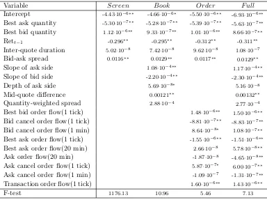
Coefficients estimates for the different information sets for the linear model are given in Table 3. The results show that for each of the three

7_{The corresponding results in the case of no transaction costs are qualitatively similar}

(24)

extended information sets beyond Screen information, the majority of the explanatory variables are statistically significant in-sample. Moreover, we can easily reject the joint hypothesis that all coefficients in each of the ex-tended information sets beyond the Screen information set are insignificant from zero on the basis of an F-test. This confirms the results in the existing literature that statistically, limit order book information does contribute to the in-sample explanation of the exchange rate. In order to check whether this apparent predictability can be translated into out-of-sample profitabil-ity, we implement the trading strategy described above using the in-sample coefficients estimates.

Table 4 reports the average out-of-sample returns of the genetic algorithm trading rules for different values of k under no transaction costs for the five sample periods.8 _{Using the empirical distribution of generated from the}

out-of-sample performance of the best 100 genetic algorithm rules, we use a t-statistic to test if the average return is statistically different from zero. The trading strategies produce high positive average daily returns for small values of the inertia parameter k (up to 6 basis points for the 2003 samples, up to 4 basis points for the March 31, 2008 sample and only for k = 0 for the April 1, 2008 sample). The t-test indicates that the average returns are significantly different from 0 in these cases. Profitability disappears as the frequency of trading decreases. In fact, after k = 12, the trading rules start generating negative out-of-sample returns during January 13-17, 2003, for

(25)

k = 16 during February 10-14, 2003 and fork = 8 during March 17-21, 2003. For the 2008 samples negative out-of-sample returns start to appear atk = 6 for the March 31 sample and at k= 2 for the April 1 sample.

A more interesting question is whether the profitability of the trading strategies remains when transaction costs are incorporated.9 Table 5 reports the out-of-sample performance of the linear model when trading on the best bid and ask prices and tests for superior predictability relative to a random walk using the Anatolyev-Gerko test.

Table 5 shows that returns drop substantially when trading at a high frequency. Small values of the inertia parameter reflect a higher number of transactions, which implies a large cumulative transaction cost that exceeds the profits from trading. As the number of transactions drops, transaction ex-penses decrease and trading rules become profitable again.10 _{Out-of-sample}

returns are positive at k ranges from 6 to 16 basis points during January 13-17, 2003, at k from 8 to 28 basis points during February 10-14, 2003 and k from 10 to 22 basis points during March 17-21, 2003. There are less pro-nounced patterns of positive returns for the 2008 sample. On March 31, only k values of 10, 20, and 22 basis points generate positive returns; there are

9_{All further results presented in the paper take transaction costs into account.}

10_{This result is in line with the findings of Knez and Ready (1996), Cooper (1999),}

(26)

positive returns on April 1 for kranging from 8 to 12 and from 16 to 20 basis points. However, it is important to note that for all samples at k = 0 and k = 2, the linear trading rule is superior to the random walk across all infor-mation sets. Although it generates negative returns, the results indicate that the random walk model loses even more based on trading with transaction costs. For each sample there are inertia values within the 10-14 basis points range that generate positive out-of-sample returns superior to the random walk model (with the exception for the March 31, 2008 sample for the Full information set).

The highest daily returns are 0.72% during January 13-17, 2003 achieved atk = 12, 1.79% during February 10-14, 2003 atk = 14, 0.89% during March 17-21, 2003 at k = 20, 1.93% during March 31, 2008 and 2.46% on April 1, at k = 12. Although these returns may look very high, there is no obvious pattern as to how to exploit them systematically due to the changing nature of the optimal inertia parameter. We address this question at the end of the section. Also, note that traders cannot invest any desired amount of capital into the trading strategy due to our restriction on the trade size.

Importantly, Table 6 shows using the t-test for zero mean that the ge-netic algorithm can handle transaction costs surprisingly well. While the inertia parameter is the only way to mediate the trading frequency for the linear trading rule, the genetic algorithm can adjust it endogenously.11 _The

trading strategy based on the genetic algorithm shows positive and signif-icant positive returns under transaction costs even for low k bands for the

11_{Note that genetic algorithm produces different trading rules for trading with no}

(27)

2003 data. Profitability vanishes though for values of k higher than 12 basis points. However, there is a big difference in 2008 data as the signs of average returns during 2008 clearly indicate the lack of a systematic pattern. Posi-tive returns are only generated across all information sets for k equal to 0, 16 or 18 basis points on March 31 and only for k = 10 basis points on April 1. Most of the average out-of-sample returns are statistically significant as indicated by the t-test but the systematic pattern of positive returns from the 2003 data has vanished.

Similar results are obtained for the trading strategy based on the “ma-jority” rule (see Table 7). There are significant and positive returns for k between 0 and 10 basis points for the 2003 samples. Most of the informa-tion sets exhibit superior performance to the random walk according to the Anatolyev-Gerko test. Returns across the 2008 samples are, however, not systematically positive and change sign from one information set to another.

(28)

too often cannot survive in-sample. The linear model strategy cannot adjust to the trading frequency in-sample and therefore it does poorly for small k but improves performance for larger k.

4.1.1. Endogenous inertia parameter

The results reported above show that the profitability of the trading rules critically depends on the value of the inertia parameter. Moreover, the op-timal value of k does not stay the same over different sample periods and across different information sets. Therefore it is important to verify prof-itability of the trading rules based on an ex-ante and systematic method for the selection of the inertia parameter. In order to do this we endogenize k in the following way. For each value of the inertia parameter, the genetic algorithm searches for the best in-sample trading rule. In-sample returns are compared with each other, while the rule with the highest return and its cor-responding value of k are used to trade out-of-sample. Note, this procedure is using information known to the trader at the time of decision making.12 The results are provided in Table 8.

Average out-of-sample returns remain positive across all information sets for the first two 2003 samples. During March 17-21, 2003, trading strategies based only on Screenand limit order book information generate positive and statistically significant returns while the other two information sets fail to generate positive profit. The samples from 2008 do not produce positive

12_{Balvers and Wu (2010) use a dynamic programming framework to design an ex-ante}

(29)

returns for any of the information sets using the endogenously determined value of k.

Table 8 presents the values of the Omega measure of performance (see Shadwick and Keating, 2002) along with Sharpe ratios. Omega is a risk-adjusted performance measure in the sense that it is a ratio of probability weighted gains to losses about a pre-specified threshold, which we take to be zero:

Ωτ =





∞

Z

τ

(1−F(x))dx



/





τ

Z

−∞

F(x)dx



,

whereF is the cumulative distribution function of returns. As such it reflects the shape of the entire return distribution and all higher moments. The table shows that both the Sharpe and Omega ratios confirm our conclusions from the cumulative returns that there is a substantial difference for all information sets between the 2003 and 2008 data. According to the Omega measure, it is clear that a general bias towards positive returns in 2003 has been replaced, in 2008, by a greater weight being found for negative returns. This is also reflected in the Sharpe ratios.

(30)

predictability consistent with an efficient market. However, standard per-formance measures may not reflect the full risks associated with the trading rules. Traders could for instance not only be exposed to market risk as mea-sured by the standard deviation of returns but also to different sources of operational risk.

(31)

end of 2007. Thus, the profitability of trading exchange rates at the highest frequency appears to have decreased substantially. This observation would be completely consistent with the AMH.

4.2. Hypothesis 2: relative performance

We now turn to Hypothesis 2 and look at the relative performance of the four information sets. In order to test the superior forecasting ability of different conditioning information, we compute the t-statistics of differences between the means of the cumulative returns. This gives us an indication of whether the differential information in each set adds value to the pre-dictions made on the basis of the most basic Screen information set. Our main conclusion is that we cannot systematically reject the null hypothesis of the superiority of the Screen information. In other words, the enhanced information sets do not appear to add significant value.

The results of the tests for the linear model are provided in Table 9. This table reports values of the Giacomini-White test of conditional superior predictive ability of each of the extended information sets versus the Screen information.

In most cases we cannot detect any superior predictive ability for any of the information sets. For most values of the inertia parameter, the extended information sets do not add significant value out-of-sample.

(32)

In Table 10, low values of the inertia parameter Screen information ap-pears to be superior to limit order book and the order flow information. There is a k range from 18 to 22 basis points, where the limit order book information dominates the Screen information. This mostly appears, how-ever, when the latter generates negative average returns (with the exception of the February 10-14, 2003 sample period).

In addition to the t-test results, we also test for conditional superior predictive ability from the information sets for the genetic algorithm based strategies. Table 11 provides the values of the Giacomini-White test statistics for the “majority” rule.

In Table 11, there are very few F-statistic, that are statistically significant. There is no clear systematic pattern among those that generate a statistically significant difference in performance between the information sets. In most cases the three information sets based on limit order book variables are not able to significantly outperform the Screen information set.

(33)

confirm that order book information has statistical in-sample explanatory power, this predictability cannot be systematically transferred into econom-ically significant profit, at least beyond that which is already in the past prices.

5. Conclusions

In this paper we examine the predictability and profitability of the U.S. dollar sterling exchange rate using limit order book information. We test formally the hypothesis of whether the limit order book information can be profitably exploited out-of-sample for five different samples during 2003 and 2008. Two approaches are used to construct trading strategies: linear regression and a genetic algorithm.

We show that there is a high level of profitability during 2003 and trad-ing strategies generate positive and significant out-of-sample returns net of transaction costs. The level of profitability appears to drop considerably if not being eliminated completely in the more recent 2008 data. This finding is in line with the Adaptive Market Hypothesis given that there has been a dramatic rise in algorithmic trading activity since 2003. To the best of our knowledge, this gain in efficiency has not yet been reported in the literature for the FX markets but would be consistent with the analysis by Hender-shott, Jones and Menkveld (2010) on the impact of algorithmic trading for equity markets.

(34)

which is visible on the screens of trading platforms. The other three are based on the limit order book and order flow information in addition to the screen information set. The information contained in the three enhanced information sets seem to be not robust enough to significantly contribute to the profitability of the trading strategies.

(35)

References

Alexander, S., 1961. Price movements in speculative markets: trends or random walks. Industrial Management Review 2, 7–26.

Allen, F., Karjalainen, R., 1999. Using genetic algorithms to find technical trading rules. Journal of Financial Economics 51, 245–271.

Anatolyev, S., Gerko, A., 2005. A trading approach to testing for predictabil-ity. Journal of Business & Economic Statistics 23, 455–462.

Arifovic, J., 1996. The behavior of the exchange rate in the genetic algorithm and experimental economies. Journal of Political Economy 104, 510–541.

Balvers, R., Wu, Y., 2010. Optimal transaction filters under transitory trad-ing opportunities: Theory and empirical illustration. Journal of Financial Markets 13, 129–156.

Bloomfield, R., O’Hara, M., Saar, G., 2005. The “make or take” decision in an electronic market: Evidence on the evolution of liquidity. Journal of Financial Economics 75, 165–199.

Cao, C., Hansch, O., Wang, X., 2009. The information content of an open limit order book. The Journal of Futures Markets 29, 16–41.

Chaboud, A., Chiquoine, B., Hjalmarsson, E., Vega, C., 2009. Rise of the machines: Algorithmic trading in the foreign exchange market. Working paper, Federal Reserve System .

(36)

Chen, S., Duffy, J., Yeh, C., 1999. Genetic programming in the coordination game with a chaotic best-responce function, in: Proceedings of the 1996 Evolutionary Programming Conference, San Diego, CA.

Chen, S., Yeh, C., 1997a. On the Coordination and Adaptability of the Large Economy: An Application of Genetic Programming to the Cobweb Model. In: Angeline, P. and Kinnear, K. (Eds.) Advances in Genetic Programming II, Cambridge MA, MIT Press.

Chen, S., Yeh, C., 1997b. Toward a computable approach to the efficient market hypothesis: An application of genetic programming. Journal of Economic Dynamics and Control 21, 1043–1063.

Chordia, T., Subrahmanyam, A., 2004. Order imbalance and individual stock returns: Theory and evidence. Journal of Financial Economics , 485–518.

Cooper, M., 1999. Filter rules based on price and volume in individual security overreaction. Review of Financial Studies 12, 901–935.

Danielsson, J., Luo, J., Payne, R., 2002. Exchange rate determination and inter-market order flow eects. Unpublished manuscript .

Della Corte, P., Sarno, L., Tsiakas, I., 2009. An economic evaluation of empirical exchange rate models. Review of Financial Studies 22, 3491– 3530.

(37)

Dworman, G., Kimbrough, S., Laing, J., 1996. On automated discovery of models using genetic programming: Bargaining in a three-agent coalitions game. Journal of Management Information Systems 12, 97–125.

Easley, D., O’Hara, M., 2010. Liquidity and valuation in an uncertain world. Journal of Financial Economics 97, 1–11.

Evans, M., Lyons, R., 2005. Meese and rogo redux: Micro-based exchange rate forecasting. American Economic Review Papers and Proceedings 95, 405–414.

Evans, M., Lyons, R., 2006. Understanding order flow. International Journal of Finance and Economics 11, 3–23.

Fama, E., Blume, M., 1966. Filter rules and stock market tradings. Jounal of Business 39, 226–241.

Foucault, T., 1999. Order flow composition and trading costs in a dynamic limit order market. Journal of Financial Markets 2, 99–134.

Froot, K., Ramadorai, T., 2005. Currency returns, intrinsic value and insti-tutional investor flows. Journal of Finance 60, 1535–1566.

Giacomini, R., White, H., 2006. Tests of conditional predictive ability. Econo-metrica 74, 1545–1578.

(38)

Granger, C., Machina, M., 2006. Forecasting and Decision Theory. In: El-liott, G. and Granger, C. and Timmermann, A. (Eds.) Handbook of Eco-nomic Forecasting, Elsevier.

Granger, C., Pesaran, H., 2000. Economic and statistical measures of forecast accuracy. Journal of Forecasting 19, 537 – 560.

Handa, P., Schwartz, R., 1996. Limit order trading. Journal of Finance 51, 1835–1861.

Handa, P., Schwartz, R., 2003. Quote setting and price formation in an order driven market. Journal of Financial Markets 6, 461–489.

Hansen, P., 2010. In-sample fit and out-of-sample fit: Their joint distribu-tion and its implicadistribu-tions for model selecdistribu-tion. Working Paper, Stanford University .

Harris, L., 1998. Optimal dynamic order submission strategies in some styl-ized trading problems. Financial Markets, Institutions & Instruments 7, 1–76.

Harris, L., Hasbrouck, J., 1996. Market vs. limit orders: the SuperDOT evi-dence on order submission strategy. Journal of Financial and Quantitative Analysis 31, 213–231.

(39)

Hellstr¨om, J., Simonsen, O., 2009. Does the open limit order book re-veal information about short-run stock price movements? Unpublished manuscript .

Hendershott, T., Jones, C., Menkveld, A., 2010. Does algorithmic trading improve liquidity? Journal of Finance 66, 1–33.

Hillman, R., Salmon, M., 2007. Intrinsic stationarity: Investigating pre-dictability in real-time forex transactions. Journal of Financial Forecasting 1, 3–43.

Huang, R., Stoll, H., 1994. Market microstructure and stock return predic-tions. Review of Financial Studies 7, 179–213.

Kaniel, R., Liu, H., 2006. What orders do informed traders use? Journal of Business 79, 1867–1913.

Kavajecz, K., 1999. A specialist’s quoted depth and the limit order book. Journal of Finance 54, 747–771.

Knez, P., Ready, M., 1996. Estimating the profits from trading strategies. Review of Financial Studies 9, 1121–1163.

Latza, T., Payne, R., 2010. Measuring the information content of limit order flows. Unpublished manuscript .

Leitch, G., Tanner, E., 1991. Economic forecast evaluation: Profits versus the conventional error measures. American Economic Review 81, 580–590.

(40)

Neely, C., Weller, P., 2001. Technical analysis and central bank intervantion. Journal of International Money and Finance 20, 949–970.

Neely, C., Weller, P., 2003. Intraday technical trading in the foreign exchange market. Journal of International Money and Finance 22, 223–237.

Neely, C., Weller, P., Dittmar, R., 1997. Is technical analysis in the for-eign exchange market profitable? Journal of Financial and Quantitative Analysis 32, 405–426.

Nix, A., Vose, M., 1992. Modeling genetic algorithms with markov chains. Annals of Mathematics and Artificial Intelligence 5, 79–88.

Parlour, C., 1998. Price dynamics in limit order markets. Review of Financial Studies 11, 789–816.

Pesaran, H., Skouras, S., 2002. Companion to Economic Forecasting. Black-well Publishers. chapter Decision-based methods for forecast evaluation. pp. 241–267.

Ranaldo, A., 2004. Order aggressiveness in limit order book markets. Journal of Financial Markets 7, 53–74.

Rime, D., Sarno, L., Sojli, E., 2010. Exchange rate forecasting, order flow and macroeconomic information. Journal of International Economics 80, 72–88.

(41)

Rosu, I., 2010. Liquidity and information in order driven markets. SSRN Working Paper series .

Sager, M., Taylor, M., 2008. Commercially available order flow data and exchange rate movements: Caveat emptor. Journal of Money, Credit and Banking 40, 583–625.

Satchell, S., Timmermann, A., 1995. An assesment of the economic value of non-linear foreign exchange rate forecasts. Journal of Forecasting 14, 477–497.

Seppi, D., 1997. Liquidity provision with limit orders and a strategic spe-cialist. Review of Financial Studies 10, 103–150.

Shadwick, W., Keating, C., 2002. A universal performance measure. Journal of Performance Measurement 6, 59–85.

(42)

[image:42.612.147.468.223.436.2]

Figure 1: Example of genetic algorithm trading rule

(43)

[image:43.612.110.497.256.532.2]

Table 1: Descriptive statistics on market liquidity

The table presents summary statistics on the liquidity of the market for the five subsam-ples. It reports the mean, standard deviation, median, minimum, maximum, and first and the third quartiles of best quantities, slopes of bid and ask sides of limit order book, the depth, inter-quote duration, and bid-ask spread. Subsamples are: January 13-17, 2003, February 10-14, 2003, March 17-21, 2003, March 31, 2008, and April 1, 2008. Best quan-tities and depth are measured in millions of pounds sterling, slopes are basis point per 100 million of currency trade, duration is in seconds and bid-ask spread is in basis points.

Variable Mean Std._Dev. Q1 Median Q3 Mean Std._Dev. Q1 Median Q3

January 13-17, 2003 February 10-14, 2003

Best bid quantity 2.80 2.53 1 2 3 3.07 5.64 1 2 3

Best ask quantity 2.90 7.45 1 2 3 3.03 5.94 1 2 3

Slope of bid side 58.69 77.87 25.92 40.00 66.67 55.53 52.43 25.00 40.00 66.67

Slope of ask side 65.35 66.08 28.57 50.00 75.00 66.71 77.11 27.77 44.44 75.00

Depth of bid side 44.43 18.45 29 44 58 48.81 34.46 26 39 56

Depth of ask side 39.63 25.86 23 32 46 34.21 14.30 25 33 42

Inter-quote dur. 2.29 16.75 0.30 1.00 2.40 1.82 3.26 0.30 0.95 2.11

Bid-ask spread 2.28 2.06 1 2 3 2.31 2.01 1 2 3

Nr. of Orders 75,135 98,785

March 17-21, 2003

Best bid quantity 2.76 2.80 1 2 3

Best ask quantity 2.84 3.19 1 2 3

Slope of bid side 75.54 101.9 30.76 50.00 83.33

Slope of ask side 85.03 98.19 33.33 57.14 100.0

Depth of bid side 40.17 15.54 28 40 51

Depth of ask side 38.22 18.58 25 33 48

Inter-quote dur. 1.84 3.33 0.31 0.92 2.22

Bid-ask spread 2.73 3.16 1 2 3

(44)

[image:44.612.110.496.160.312.2]

Table 1 continued

Variable Mean Std._Dev. Q1 Median Q3 Mean Std._Dev. Q1 Median Q3

March 31, 2008 April 1, 2008

Best bid quantity 3.93 4.06 2 3 5 4.00 4.31 2 3 5

Best ask quantity 3.80 4.63 2 3 5 4.01 6.23 2 3 5

Slope of bid side 20.89 14.54 12.50 17.64 25.00 19.52 12.05 11.76 16.66 25.00

Slope of ask side 21.52 14.31 13.33 18.18 25.00 20.26 13.50 12.50 16.66 25.00

Depth of bid side 79.87 27.69 61 78 94 89.56 32.82 70 85 100

Depth of ask side 72.62 33.12 48 67 89 80.64 32.60 55 79 98

Inter-quote dur. 0.10 0.32 0.01 0.03 0.09 0.09 0.28 0.01 0.03 0.08

Bid-ask spread 2.53 1.21 2 2 3 2.49 1.22 2 2 3

(45)

[image:45.612.114.488.206.433.2]

Table 2: Number of indicative trades

This table provides the number of times the mid-quote of the exchange rate goes outside thek-band for different values of k. When the exchange rate crosses the k-band, trading rules re-evaluate positions taken in the exchange rate. Trade occurs when the trading rule requires a change in the direction of the position. k is measured in basis points.

k January₂₀₀₃13-17, February₂₀₀₃10-14, March₂₀₀₃17-21, March₂₀₀₈31, April₂₀₀₈1,

0 16,889 22,468 19,654 19,263 12,005

2 1,745 2,775 1,366 1,255 744

4 497 877 443 421 221

6 252 425 215 218 108

8 144 251 140 128 71

10 97 166 99 83 39

12 69 117 64 58 35

14 59 83 45 46 23

16 41 65 34 37 17

18 31 48 24 29 12

20 23 35 22 20 11

22 19 31 22 18 13

24 15 25 21 18 7

26 15 23 15 12 6

28 11 15 14 12 4

(46)

[image:46.612.113.497.289.576.2]

Table 3: Linear model parameters estimates

This table presents coefficient estimates from the linear regression of one-step ahead returns on different conditioning variables. The estimation period is the first half of the week commencing on January 13, 2003. The “Screen” column contains estimates of the variables from the Screen information set, “Book” corresponds to the limit order book information set, “Order” denotes order flow information and “Full” provides results for the combined information set. The table does not include variables that are not significant in any of the information sets. The F-test row presents F-statistic values for testing the joint significance of all variables added in addition to theScreeninformation set variables (in the “Screen” column the usual F-statistic for significance of the regression is given). ∗ and∗∗indicate significance at the 5% and 10% levels.

Variable Screen Book Order F ull

Intercept -4.43·10−6∗∗ _-4.66_·₁₀−6∗ _-5.50_·₁₀−6∗∗ _-6.93_·₁₀−6∗∗

Best ask quantity -5.30·10−7∗∗ _-5.28_·₁₀−7∗∗ _-5.39_·₁₀−7∗∗ _-5.63_·₁₀−7∗∗

Best bid quantity 1.12·10−6∗∗ _9.33_·₁₀−7∗∗ _1.01_·₁₀−6∗∗ _8.66_·₁₀−7∗∗

Rett−1 -0.296∗∗ -0.295∗∗ -0.312∗∗ -0.311∗∗

Inter-quote duration 5.02·10−8 _7.42_·₁₀−8 _9.62_·₁₀−8 _1.08_·₁₀−7

Bid-ask spread 0.0116∗∗ _0.0129∗∗ _0.0117∗∗ _0.0129∗∗

Slope of ask side 1.08·10−4∗∗ 1.17·10−4∗∗

Slope of bid side -2.20·10−4∗∗

-2.30·10−4∗∗

Depth of ask side 5.69·10−8∗

5.16·10−8

Mid-quote difference 0.00121∗∗ _0.00132∗∗

Quantity-weighted spread 2.88·10−4 _2.77_·₁₀−4

Best bid order flow(1 tick) 1.48·10−6∗∗ 1.50·10−6∗∗

Bid cancel order flow(1 tick) -8.81·10−7∗∗

-8.83·10−7∗∗

Bid cancel order flow(1 min) 8.64·10−8∗

1.08·10−7∗∗

Best ask order flow(1 tick) -1.55·10−6∗∗ _-1.51_·₁₀−6∗∗

Best ask order flow(20 min) 2.66·10−8 _5.78_·₁₀−8∗∗

Ask order flow(20 min) -1.87·10−8 _-4.65_·₁₀−8∗∗

Ask cancel order flow(1 tick) 5.87·10−7∗

6.00·10−7∗∗

Ask cancel order flow(1 min) -1.09·10−7 _-1.31_·₁₀−7∗∗

Transaction order flow(1 tick) 1.60·10−6∗∗ _1.43_·₁₀−6∗∗

(47)

[image:47.612.243.486.183.643.2]

(48)

[image:48.612.144.376.257.553.2]

(49)

[image:49.612.244.485.183.650.2]

(50)

[image:50.612.143.377.257.552.2]

(51)

[image:51.612.234.485.181.646.2]

(52)

[image:52.612.146.377.258.553.2]

(53)

[image:53.612.258.496.185.634.2]

(54)

[image:54.612.146.376.259.553.2]

(55)

(56)

[image:56.612.113.497.312.556.2]

Table 9: Relative performance of the linear model

The table presents values of Giancomini-White test statistics for comparing the relative out-of-sample performance of the linear model based on three information sets against the Screen information. The linear regression coefficients are estimated using in-sample and return predictions are formed for the out-of-sample period. A simple binary trading rule is implemented based on the return predictions. Transaction costs are reflected in the bid-ask spread as trading is based on best bid and ask limit orders. kis the threshold value for the trading band and measured in basis points. Columns “Book-Screen” contains statistics for relative performance of the limit order book versus theScreeninformation, “Order-Screen” compares the order flow versus the Screeninformation and “Full-Screen” corresponds to the combined information set versus theScreeninformation. Asterisks indicate significant values at 5% level; ∗corresponds to the cases where the Screen information outperforms the corresponding information set, ∗∗presents the opposite situation.

January 13-17, 2003 February 10-14, 2003 March 17-21, 2003

k _ScreenBook- Order-_Screen _ScreenFull- _ScreenBook- Order-_Screen _ScreenFull- _ScreenBook- Order-_Screen _Screen

Full-0 5.79 2.20 7.29∗∗ 16.70∗∗ 1.71 22.02∗ 6.72∗∗ 41.71∗ 2.46

2 2.17 4.52 1.58 1.46 3.33 1.57 1.46 5.62 6.17∗

4 6.04∗ 1.54 4.77 1.01 3.42 0.39 0.59 1.46 1.78

6 2.03 0.13 0.45 6.38∗ _0.38 _4.13 _0.50 _1.89 _1.89

8 1.19 3.39 1.92 2.01 2.66 0.51 0.69 0.24 0.74

10 N/A N/A 1.06 0.92 2.75 0.59 0.15 0.13 0.44

12 N/A 1.95 1.46 0.40 N/A 0.40 0.08 N/A 0.13

14 N/A N/A N/A 1.59 N/A 1.59 2.34 2.39 3.95

16 N/A 0.82 N/A 0.49 N/A 0.49 N/A 1.09 2.38

18 N/A 2.71 0.82 N/A 2.34 2.34 N/A 2.97 2.97

20 N/A N/A 2.71 0.77 N/A 1.71 2.47 2.02 4.82

22 N/A N/A N/A N/A N/A N/A 2.23 N/A 2.23

24 N/A N/A N/A N/A 2.89 3.43 N/A N/A 2.11

26 N/A N/A N/A 1.95 N/A 1.72 N/A 2.00 2.00

28 N/A N/A N/A N/A N/A N/A N/A N/A N/A

(57)

[image:57.612.167.434.158.400.2]

Table 9 continued

March 31, 2008 April 1, 2008

k _ScreenBook- Order-_Screen _ScreenFull- _ScreenBook- Order-_Screen _Screen

Full-0 5.79 2.20 7.29∗∗ 10.14∗ 47.01∗∗ 19.23∗∗

2 2.17 4.52 1.58 0.02 4.09 6.95∗∗

4 6.04∗ 1.54 4.77 2.92 3.39 0.47

6 2.03 0.13 0.45 N/A 2.62 1.78

8 1.19 3.39 1.92 N/A 1.52 2.55

10 N/A N/A 1.06 N/A 0.04 0.08

12 N/A 1.95 1.46 N/A 5.34 2.49

14 N/A N/A N/A N/A 3.75 3.75

16 N/A 0.82 N/A N/A 0.77 0.77

18 N/A 2.71 0.82 N/A 0.12 0.12

20 N/A N/A 2.71 N/A 0.06 1.41

22 N/A N/A N/A N/A 0.79 3.07

24 N/A N/A N/A N/A 1.83 1.83

26 N/A N/A N/A N/A 0.14 0.14

28 N/A N/A N/A N/A 2.00 N/A

(58)

[image:58.612.113.499.326.567.2]

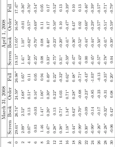
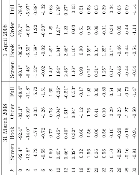
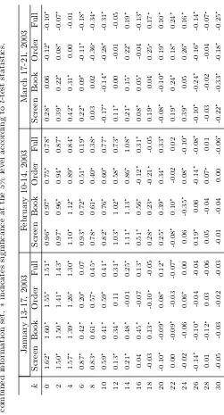
Table 10: Relative performance of the genetic algorithm model

The table presents values of pairedt-test statistics for comparing the relative out-of-sample performance of the genetic algorithm model based on three information sets against the Screen information. The in-sample period (the first half of the sample) is then used to select the best performing trading rule and this rule is used to trade out-of-sample (the second half of the sample). The exercise is repeated 100 times to generate the empirical distribution of cumulative returns. Transaction costs are reflected in the bid-ask spread as trading is based on the best bid and ask limit orders. k is the threshold value for the trading band and measured in basis points. Columns “Book-Screen” contains statistics for relative performance of the limit order book versus theScreeninformation, “Order-Screen” compares the order flow versus the Screeninformation and “Full-Screen” corresponds to the combined information set versus theScreeninformation. Asterisks indicate significant values at 5% level; ∗ corresponds to the cases where theScreen information outperforms the corresponding information set, ∗∗presents the opposite situation.

Full-0 -0.46 -1.17 -1.54 0.12 -2.72∗ -2.09∗ -3.84∗ -6.99∗ -7.61∗

2 -0.22 -2.37∗ _-1.85∗ _-0.20 _-0.55 _-1.59 _-3.49∗ _-5.58∗ _-9.88∗

4 -2.73∗ _-3.34∗ _-2.95∗ _0.22 _-2.82∗ _-3.04∗ _-2.20∗ _-5.21∗ _-6.58∗

6 -3.05∗ -4.51∗ -5.88∗ -2.52∗ -3.98∗ -7.71∗ -2.26∗ -4.68∗ -5.92∗

8 -1.43 -1.85∗ -2.57∗ -2.31∗ -5.01∗ -6.69∗ -0.09 -4.43∗ -4.12∗

10 -1.88∗ -0.03 -1.79∗ -0.77 -2.98∗ -0.61 0.44 -1.75∗ -2.13∗

12 2.09∗∗ _-0.11 _1.93∗∗ _-0.15 _-5.35∗ _-3.54∗ _-1.26 _-1.66 _-2.35∗

14 3.01∗∗ _-2.20∗ _0.51 _0.26 _-2.69∗ _-0.45 _-0.86 _0.14 _-0.28

16 5.18∗∗ -1.58 1.12 0.66 -8.66∗ -2.30∗ -0.47 -2.16∗ -3.85∗

18 2.55∗∗ -1.27 -0.32 -0.72 -8.12∗ -4.94∗ -2.70∗ 1.02 -0.31

20 0.11 3.09∗∗ 3.78∗∗ 2.36∗∗ 2.00∗∗ 1.49 -0.41 3.87∗∗ 2.68∗∗

22 -1.97∗ _-0.66 _-1.57 _3.37∗∗ _1.19 _1.92∗∗ _0.69 _-0.23 _0.74

24 -0.73 1.73∗∗ 0.43 -7.24∗ 0.31 -2.50∗ -6.34∗ -1.94∗ -3.97∗

26 0.84 2.07∗∗ 2.16∗∗ -2.69∗ -6.71∗ -5.30∗ -2.38∗ -1.06 -0.82

28 -3.00∗ 0.38 -1.36 -1.77∗ 0.58 -0.89 0.23 -0.32 -0.80

(59)

[image:59.612.167.433.159.400.2]

Table 10 continued

March 31, 2008 April 1, 2008

Full-0 -1.96∗ -2.63∗ -3.58∗ -2.09∗ -6.09∗ -4.20∗

2 -1.56 -1.82∗ -1.70∗ 0.51 -22.85∗ -22.67∗

4 -5.96∗ -4.50∗ -3.26∗ 1.71∗∗ -4.88∗ -3.84∗

6 2.18∗∗ _2.54∗ _0.99 _0.84 _1.58 _2.66∗∗

8 -0.68 -2.30∗ -1.07 0.60 -1.63 -3.65∗

10 -0.02 -1.75∗ -0.34 -1.39 0.52 0.11

12 0.78 0.88 1.46 2.52∗∗ -1.04 -0.76

14 0.98 -2.80∗ _-5.26∗ _-3.03∗ _-1.62 _0.27

16 -1.97∗ _-4.11∗ _-2.79∗ _2.98∗∗ _2.43∗∗ _-0.86

18 2.33∗∗ -0.82 0.11 1.33 5.22∗∗ 5.77∗∗

20 3.32∗∗ 2.30∗∗ -0.14 0.87 5.39∗∗ 6.94∗∗

22 -2.11∗ -1.28 -0.76 -3.65∗ -4.41∗ -3.31∗

24 2.71∗∗ _-1.84∗ _-2.30∗ _-0.45 _-1.70∗ _-1.02

26 -0.42 -1.08 1.27 -0.82 -0.80 -1.89∗

28 -0.15 -2.01∗ -1.20 6.17∗∗ 4.64∗∗ 1.33

(60)

[image:60.612.111.499.326.569.2]

Table 11: Relative performance of the GA “majority” trading rule

The table presents values of Giancomini-White test statistics for comparing the relative out-of-sample performance of the “majority” rule based on three information sets against theScreeninformation. 99 independent runs of the genetic algorithm have been performed to select the best in-sample trading rules. The “majority” rule produces a “buy” (“sell”) signal if the majority of the 99 best in-sample rules produce a “buy” (“sell”) signal. This combined rule is then used to trade out-of-sample. Transaction costs are reflected in the bid-ask spread as trading is based on the best bid and ask limit orders. kis the threshold value for the trading band and measured in basis points. Columns “Book-Screen” contains statistics for relative performance of the limit order book versus the Screen information, “Order-Screen” compares the order flow versus theScreen information and “Full-Screen” corresponds to the combined information set versus theScreeninformation. Asterisks indi-cate significant values at 5% level;∗corresponds to the cases where theScreeninformation outperforms the corresponding information set, ∗∗presents the opposite situation.