Quantifying the uncertainty in change points

Original citation:

Nam, Christopher F. H., Aston, John A. D. and Johansen, Adam M.. (2012) Quantifying

the uncertainty in change points. Journal of Time Series Analysis, Volume 33 (Number

5). pp. 807-823. ISSN 0143-9782

Permanent WRAP url:

http://wrap.warwick.ac.uk/44378

Copyright and reuse:

The Warwick Research Archive Portal (WRAP) makes this work by researchers of the

University of Warwick available open access under the following conditions. Copyright ©

and all moral rights to the version of the paper presented here belong to the individual

author(s) and/or other copyright owners. To the extent reasonable and practicable the

material made available in WRAP has been checked for eligibility before being made

available.

Copies of full items can be used for personal research or study, educational, or

not-for-profit purposes without prior permission or charge. Provided that the authors, title and

full bibliographic details are credited, a hyperlink and/or URL is given for the original

metadata page and the content is not changed in any way.

Publisher’s statement:

Article is published under the Wiley OnlineOpen scheme and information on reuse rights

can be found on the Wiley website:

http://olabout.wiley.com/WileyCDA/Section/id-406241.html

A note on versions:

The version presented in WRAP is the published version or, version of record, and may

be cited as it appears here.

Quantifying the uncertainty in change points

Christopher F. H. Nam

John A. D. Aston

and Adam M. Johansen

Quantifying the uncertainty in the location and nature of change points in time series is important in a variety of applications. Many existing methods for estimation of the number and location of change points fail to capture fully or explicitly the uncertainty regarding these estimates, whilst others require explicit simulation of large vectors of dependent latent variables. This article proposes methodology for approximating the full posterior distribution of various change point characteristics in the presence of parameter uncertainty. The methodology combines recent work on evaluation of exact change point distributions conditional on model parameters via finite Markov chain imbedding in a hidden Markov model setting, and accounting for parameter uncertainty and estimation via Bayesian modelling and sequential Monte Carlo. The combination of the two leads to a flexible and computationally efficient procedure, which does not require estimates of the underlying state sequence. We illustrate that good estimation of the posterior distributions of change point characteristics is provided for simulated data and functional magnetic resonance imaging data. We use the methodology to show that the modelling of relevant physical properties of the scanner can influence detection of change points and their uncertainty.

Keywords: Change points; finite Markov chain imbedding; functional magnetic resonance imaging; hidden Markov models; sequential Monte Carlo; segmentation.

1. INTRODUCTION

Detecting and estimating the number and location of change points in time series is becoming increasingly important as both a theoretical research problem and a necessary part of applied data analysis. Originating in the 1950s in a quality control setting (Page, 1954), there are numerous existing approaches, both parametric and non-parametric, often requiring strong assumptions on the type of changes that can occur and the distribution of the data. We refer the reader to Chen and Gupta (2000); Eckleyet al.(2011) for good overviews of some of these existing methods. It is also worth noting that change point problems appear under various names including segmentation, novelty detection, structural break identification, and disorder detection. These approaches however, typically fail to fully capture uncertainty in the number and location of these change points. For example, model selection and optimal segmentation-based techniques (e.g. Yao, 1988; Daviset al., 2006) rely on asymptotic arguments on providing consistent estimates of the number of change points present, whilst others assume the number of change points to be known to consider the uncertainty regarding the locations of these change points (see Stephens, 1994, Chib, 1998). Those methods which do fully characterize the uncertainty involved typically require simulation of large vectors of correlated latent variables. Chen and Liu (1996) also provide a sampling algorithm to obtain Bayesian classification probabilities with respect to which latent state the observations belongs to.

This article proposes a methodology which fully quantifies the uncertainty of change points for an observed time series, without estimating or simulating the unobserved state sequence. Avoiding simulation of a latent state sequence is desirable in some settings and this is one significant motivation of the technique proposed in this article.

Our proposed methodology is based on three areas of existing work. We model our observed time series and consider change points in a Hidden Markov Model (HMM) framework. HMMs and the general use of dependent latent state variables are widely used in change point estimation (Chib, 1998; Fearnhead, 2006; Fearnhead and Liu, 2007). In these approaches, each state of the underlying chain represents a segment of data between change points and thus a change point is said to occur when there is a change in state in the underlying chain. The underlying chain is constructed so that there are only two possible moves; either stay in the same state (no change point has occurred), or move to the next state in the sequence, corresponding to a new segment and thus a change point has occurred. Interest now lies predominantly in determining the latent state sequence [usually through simulation, e.g. by Markov Chain Monte Carlo (MCMC)], so as to determine the relevant change point characteristics. We note that under the framework of Chib (1998), the number of change points is assumed to be known since this is related to the number of states of the imposed HMM. However, this is quite restrictive and makes sense only in those settings in which returns to a previously visited segment and state is regarded as impossible.

We consider an alternative approach by using HMMs in their usual context, where each state represents different data generating mechanisms [e.g. the ‘good’ and ‘bad’ states when using a Poisson HMM to model the number of daily epileptic seizure counts

a_{University of Warwick}

*Correspondence to: Department of Statistics, University of Warwick, Coventry, CV4 7AL, UK. †_{E-mail: j.a.d.aston@warwick.ac.uk}

First version received May 2011 Published online in Wiley Online Library: 14 March 2012

(Albert, 1991)] and returning to previously visited states is possible. This allows the number of change points to be unknowna priori

and inferred from the data. We do at present assume that the number of different states is known although the method can be extended to the more general case. This latter point seems less restrictive in a change point context than assuming the number of change points to be known given the quantities of interest. By modelling the observations under a HMM framework, we are able to compute exactly the likelihood via the Forward equations (e.g. Rabiner, 1989), which do not require the underlying state sequence to be estimated or sampled.

We also consider a generalized definition of change points corresponding to asustainedchange in the underlying state sequence. This means that we are looking for runs of particular states in the underlying state sequence: determining that a change point to a particular regime has occurred when a particular sequence of states is observed. We employ finite Markov chain imbedding (FMCI) (Fu and Koutras, 1994; Fu and Lou, 2003), an elegant framework which allows distributions regarding run and pattern statistics to be efficiently calculated exactly in that they are not subject to sampling or approximation error.

The above techniques allow exact change point distributions to be computed. However, these distributions are conditional on the model parameters. In practice, it is common for these parameters to be treated as known, with maximum likelihood estimates being used. In most applications where parameters are estimated from the data itself, it is desirable to account for parameter uncertainty in change point estimates. If a Bayesian approach to the characterization of changes is employed, then it would also seem desirable to take a Bayesian approach to the characterization of parameter uncertainty. Recent Bayesian change point approaches have dealt with model parameter uncertainty by integrating the parameters out in some fashion to ultimately sample from the joint posterior of the location and number of change points, usually achieved by also sampling the aforementioned latent state sequence (Fearnhead, 2006; Chib, 1998). However, this introduces additional sampling error into the change point estimates and requires the simulation of the underlying state sequence which is often long and highly correlated — and thus hard to sample efficiently. We consider model parameter uncertainty by sampling from the the posterior distribution of the model parameters via sequential Monte Carlo (SMC), without simulating the latent state sequences as we use the exact computation of the likelihood under a HMM framework. This approach introduces sampling error only in the model parameters and retains, conditionally, the exact change point distributions: we will show that this amounts to a Rao-Blackwellized form of the estimator.

Quantifying the uncertainty in change point problems is an often overlooked but nevertheless important aspect of inference. Whilst, quite naturally, more emphasis has typically been placed on detection and estimation in problems, quantifying the uncertainty of change points can lead to a better understanding of the data and the system generating the data. Whenever estimates are provided for the location of change points, we should be interested in determining how confident we can be about these estimates, and whether other change point configurations are plausible. In many situations it may be desirable to average over models rather than choosing a most probable explanation. Alternatively, we may want to assess the confidence we have in the estimate of the number of change points and if there is any substantial probability of any other number of change points having occurred. In addition, different change point approaches can often lead to different estimates when applied to the same time series; this motivates the assessment of the performance and plausibility of these different approaches and their estimates. Quantifying the uncertainty provides a means of so doing.

The exact change point distributions computed via FMCI methodology (Astonet al., 2011) already quantify the residual uncertainty given both the model parameters and the observed data. However, this conditioning on the model parameters is typically difficult to justify. It is important to consider also parameter uncertainty because the use of different model parameters can give quite different change point results and thus conclusions. This effect becomes more important when there are several different competing model parameter values which provide equally-plausible explanations of the data. By considering model parameter uncertainty within the quantification of uncertainty for change points, we are able to account for all types of change point behaviour under a variety of model parameter scenarios and thus fully quantify the uncertainty regarding change points. This will be seen to be especially true in the analysis of functional magnetic resonance imaging (fMRI) time series.

When analysing fMRI data, it is common to assume that the data arises from a known experimental design (Worsleyet al., 2002). However, this assumption is very restrictive particularly in experiments common in psychology where the exact timing of the expected reaction is unknown, with different subjects reacting at different times and in different ways to an equivalent stimulus (Lindquistet al., 2007). Change point methodology has therefore been proposed as a possible solution to this problem, where the change points effectively act as a latent design for each time series. Significant work has been done in designing methodology for these situations for the at-most-one-change situation using control chart type methods (Lindquistet al., 2007; Robinsonet al., 2010). Using the methodology developed in this article, we are able to define an alternative approach based on HMMs that allows not only multiple change points to be taken into account, but also the inclusion of an autoregressive (AR) error process assumptions and detrending within a unified analysis. These features need to be accounted for in fMRI time series (Worsleyet al., 2002) and will be shown to have an effect on the conclusions that can be drawn from the associated analysis.

The remainder of this article has the following structure: Section 2 details the statistical background of the methodology which is proposed in Section 3. This methodology is applied to both simulated and fMRI data in Section 4. We conclude in Section 5 with some discussion of our findings.

2. BACKGROUND

Let y1;y2;. . .;yn be an observed non-stationary time series with respect to a varying second order structure. One particular framework for modelling such a time series is via HMMs where the observation processfYtgt>0is conditionally independent given an

unobserved underlying Markov chain fXtgt>0. The states of the underlying chain correspond to different data generating mechanisms, with each state characterized by a collection of parameter values. The methods presented in this article can be applied to general finite state HMMs (including Markov switching models) with finite dependency on previous states of the underlying chain. This class of HMMs are of the form:

ytjy1:t1;x1:tfðytjxtr:t;y1:t1;hÞ (Emission)

pðxtjx1:t1;y1:t1;hÞ ¼pðxtjxt1;hÞ; t¼1;. . .;n (Transition).

ð1Þ

Given the set of model parameters h, the observation at time t¼1;. . .;n; yt has emission density dependent on previous observations y1:t1 and r previous latent states, xtr;. . .;xt1. For any generic sequence, u1;u2;. . . we use the notation ut1:t2 ¼ ðut1;ut1þ1;. . .;ut2Þ. The underlying states are assumed to follow a first order Markov chain (although standard embedding

arguments would in principle allow generalization to anmth order Markov chain) and takes values in the finite state spaceXX. The components ofhare dependent on the particular general HMM but typically consist of transition probabilities for the underlying Markov chain, and parameters relating to the emission density. For good overviews of HMMs, we refer the reader to MacDonald and Zucchini (1997); Cappe´et al.(2005).

A common definition within an HMM framework is that a change point has occurred at timetwhenever there is a change in the underlying chain, that isxt1 6¼ xt. This definition is currently adopted in existing works such as Chib (1998); Hamilton (1989); Durbin et al.(1998); Fearnhead (2006). However, we consider a slightly more general definition; a change point to a regime occurs at timet

when the change in the underlying chain persists for at least k time periods. That is xt1 6¼ xt ¼ . . . ¼ xtþj where jk1. Although this definition can be interpreted as an instance of the simpler definition defined on a suitably expanded space, it is both easier to interpret and computationally convenient to make use of this explicit form. The motivation for this generalized definition is that there are several applications and scenarios in which a sustained change is required before a change to a new regime is said to have occurred. Typical examples include Economics where a recession is said to have occurred when there are at least two consecutive negative growth (contraction) states and thusk¼2, or in Genetics where a specific genetic phenomena, for example a CpG island (Aston and Martin, 2007), is at least a few hundred bases long (e.g.k¼1000) before being deemed in progress. The standard change point definition can be recovered by settingk¼1.

Interest often lies in determining the time of a change point and the number of change points occurring within a time series. Let

M(k)andsðkÞ _{¼ ðs}ðkÞ

1 ;. . .;s

ðkÞ

MðkÞÞbe variables denoting the number and times of change points respectively. Given a vectors

(k)

we use

t 2 s(k)to indicate that one of the elements ofs(k)is equal tot: ift 2 s(k);then$j 2 f1;. . .;M(k)gsuch thatsð_jkÞ ¼ t. The goal of this article is to quantify the uncertainty in estimates of these characteristics by estimating:

PðMðkÞ¼mjy1:nÞ; m¼0;1;2;3;. . .; ð2Þ

andP sðkÞ3tjy1:n

ð3Þ

wherePðsðkÞ _{3 tjy}

1:nÞ ¼ PmPðMðkÞ ¼ mjy1:nÞPmi¼1Pðs

ðkÞ

i ¼ tjy1:n;MðkÞ ¼ mÞ. That is, the probability distribution of the number of changes and the marginal posterior probability that a change point occurs at any particular time.

2.1. Exact change point distributions using FMCI

Under this generalized change point setting and conditioned on a particular model parameter settingh, it is possible to compute exact distributions regarding change point characteristics (Astonet al., 2011). That is, it is possible to computePðsðkÞ_3tjy

1:n;hÞand

PðMðkÞ _{¼ mjy}

1:n;hÞexactly, where exact means that they are not subject to sampling or approximation error.

The generalized definition of a change point consequently motivates that we are looking for runs of a minimum lengthkin the underlying chain, where a run of lengthkin states 2 XXiskconsecutive occurrences ofs. That is,xt ¼ s ¼ xtþ1 ¼ . . . ¼ xtþk1, and in this instance, ifxt16¼sthe run of desired lengthkhas occurred at timet+k1. Thus to consider whether a change point

has occurred by timet;we can reformulate this problem as determining whether a run of length exactlykhas occurred at time

t+k1 in the underlying chain.

LetsðukÞdenote the time of theuth change point withu1. We can decompose the change point probability of interest into:

PðsðkÞ_3tjy

1:n;hÞ ¼

X

m

PðMðkÞ¼mjy1:n;hÞ

Xm

u¼1 PðsðkÞ

u ¼tjMðkÞ¼m;y1:n;hÞ ð4Þ

¼ X

u¼1;2;...

PðsðkÞ

u ¼t;MðkÞujy1:n;hÞ: ð5Þ

The event of theuth change point occurring at timetcan be re-expressed as a quantity involving runs, specifically: whether the

uth run of minimum lengthkhas occurred at timet+k1. LetWs(k,u) denote the waiting time for theuth occurrence of a run of minimum lengthkin states 2 XX. ThusWs(k,u)¼tdenotes that at timet, theuth occurrence of a such a run occurs.W(k,u) similarly denotes the waiting time for theuth occurrence of a run in any states 2 XXof at least lengthk. If change points into a certain regime were of interest,Ws(k,u) wheres 2 XXis the state defining the regime of interest, is of greater interest. By re-expressing the

uth change point event as the waiting time for the uth occurrence of a run, it is thus possible to compute the corresponding probabilities:

PðsðkÞ

u ¼tjy1:n;hÞ ¼PðWðk;uÞ ¼tþk1jy1:n;hÞ: ð6Þ It is possible to compute exactly the distribution of waiting time statistics, namelyP(W(k,u)t|h,y1:n), via FMCI (Fu and Koutras, 1994; Fu and Lou, 2003). FMCI introduces several auxiliary Markov processes,fZð_t1Þ;Z_tð2Þ;Zð_t3Þ;. . .gwhich are defined over the common state spaceXð_ZkÞ ¼ XX f1;0;1;. . .;kg.XðZkÞis an expanded version ofXXwhich consists of tuples (Xt,j) where the new variable

j¼ 1;0;1;2. . .;kindicates the progress of any potential runs. The auxiliary processes are constructed such that theuth process corresponds to the conditional Markov chain for finding a run of lengthk, conditional on the fact thatu1 runs of length at leastk

have already occurred multiplied by the conditional probability ofu1 runs having occurred.

The states of the auxiliary Markov chains can loosely be categorized into three categories: continuation (j¼ 1), run in progress (j¼0;1;2;. . .;k1) and absorption (j¼k). Absorption states denote that the run of required length has occurred, the run in progress states are fairly self explanatory, and continuation states denote when the (u1)th run is still in progress (its length exceeds the required length ofk) and needs to end before the occurrence of the newuth run can be considered. The transition probabilities of these auxiliary Markov chainsfZ_tð1Þ;Z_tð2Þ;Z_tð3Þ;. . .gare obtained deterministically from those of the original Markov chainfXtg. In an HMM framework, the time-inhomogeneous posterior transition probabilities are used to account for all possible state sequences given the observed time series.

Thus to determine whether the specific occurrence of a run has occurred by a specific time, we simply need to determine if the corresponding auxiliary Markov chain has reached the absorption set,A, the set of all absorption states, by the specified time. The corresponding probability can thus be computed by standard Markov chain results. This leads to computing the probability of the

uth change point probability.

PðWðk;uÞ tþk1jy1:n;hÞ ¼PðZðtþuÞk12Ajy1:n;hÞ ð7Þ

PðsðkÞ

u ¼tjy1:n;hÞ ¼PðWðk;uÞ ¼tþk1jy1:n;hÞ ð8Þ

¼PðWðk;uÞ tþk1jy1:n;hÞ PðWðk;uÞ tþk2jy1:n;hÞ: ð9Þ

The distribution of the number of change points can also be computed from these waiting time distributions:

PðMðkÞ¼mjy1:n;hÞ ¼PðWðk;mÞ njy1:n;hÞ PðWðk;mþ1Þ njy1:n;hÞ ð10Þ

In general, this FMCI approach allows for exact computation of distributions for other change point characteristics such as the probability of a change within a given time interval and the distribution of the regime durations. This thus provides a flexible methodology in capturing the uncertainty of change point problems.

These distributions of change point characteristics are conditioned on the model parametersh. However, it is typical forhto be unknown, and subject to error and uncertainty (e.g. estimation error). In order to fully consider uncertainty in change points, it is necessary to consider also the uncertainty of the parameters. We can account for model parameters via the use of SMC samplers.

2.2. SMC samplers

To deal with parameter uncertainty, we adopt a Bayesian approach by integrating out the model parameters to obtain a marginal posterior distribution on the change point quantities alone. However, it is not feasible to perform this integration analytically for the models of interest.

Sequential Monte Carlo methods are a class of simulation algorithms for sampling from a sequence of related distributions, fpbgBb¼1, via importance sampling and resampling techniques. Common applications of these methods in Statistics, Engineering and related disciplines include sampling from a sequence of posteriors as data becomes available and the particle filter for approximating

the optimal filter (to obtain the distribution of the underlying state sequence as observations become available) in general (typically continuous) state space nonlinear and non-Gaussian HMMs (Gordonet al., 1993); see Doucet and Johansen (2011) for a recent survey. We do not use SMC to infer the underlying state sequence in our particular context because the state sequence is ultimately of little interest to us and we can calculate quantities of interest marginally.

The standard application of SMC techniques requires that the sequence of distributions of interest are defined on a sequence of increasing state spaces and that one is interested in only particular marginal distributions. SMC samplers (Del Moralet al., 2006) are a class of SMC algorithms in which a collection of auxiliary distributions are introduced to allow the SMC technique to be applied to essentially arbitrary sequences of distributions defined over any sequence of spaces. One use of this framework is to allow SMC to be used when one has a sequence of related distributions defined over a common space. The innovation is to expand the space under consideration and introduce auxiliary distributions which admit the distributions of interest as marginals. This is done by the introduction of a collection of Markov kernels,fLbgwith distributions of interestfpbðxbÞgbeing formally augmented with these Markov kernels to producef~pbgwith~pbðx1:bÞ:¼pbðxbÞQbj¼11Ljðxjþ1;xjÞ.

Given a weighted sample fWi b1;h

i

b1g which is properly weighted to target pb1ðhb1Þ the SMC sampler with proposal kernel Kbðhib1;hbiÞ is used, leading to a sample fWib1;ðh

i

b1;hibÞg which is properly weighted for the distribution

pb1ðhib1ÞKbðhib1;h

i

bÞ. Given any backward kernel, Lb1ðhb;hb1Þ which satisfies an appropriate absolute continuity requirement, one can adjust the weights of the sample such that it is instead properly weighted to target the distribution pbðhbÞLb1ðhb;hb1Þby multiplying those weights by an appropriate incremental weight (settingWib/Wbi1w~bðhib1;h

i

bÞ). These incremental weights are

~ wbðhib1;h

i bÞ ¼

pbðhibÞLb1ðhib;hib1Þ

pb1ðhib1ÞKbðhib1;hibÞ

; ð11Þ

whereLb1ðhib;hib1Þis a backwards Markov kernel. Del Moralet al.(2006) established that the optimal choice of backward kernel, if resampling is conducted every iteration, is

Lopt_b1ðhb;hb1Þ ¼

pb1ðhb1ÞKbðhb1;hbÞ

R

pb1ðh0b1ÞKbðh0b1;hbÞdh0b1

;

the integral in the denominator is generally intractable and it is necessary to find approximations (the use of which increases the variance of the estimator but does not introduce any further approximation). Whenpb-invariant MCMC kernels are used for Kb a widely-used approximation of this optimal quantity can be obtained by noting that consecutive distributions in the sequence are in some sense similar,pb1pband by replacingpb1withpbin the optimal backward kernel, we obtain:

Ltr

b1ðhb;hb1Þ ¼

pbðhb1ÞKbðhb1;hbÞ

R

pbðh0b1ÞKbðh0b1;hbÞdh0b

¼pbðhb1ÞKðhb1;hbÞ

pbðhbÞ

;

by thepb-invariance ofKb. This leads to the convenient incremental weight expression:

~

wbðhib1;hibÞ ¼

pbðhib1Þ

pb1ðhib1Þ

: ð12Þ

A standard use of this framework is to provide samples from a complex distribution by sampling first from a tractable distribution and then employing mutation and selection operations to provide a sample which is appropriately weighted for approximating a complex, intractable distribution of interest. This particular application, with no selection coincides with the Annealed Importance Sampling algorithm of Neal (2001).

In the change point problems described here, the objective is to approximate the posterior distribution of the model parameters,

p(h|y1:n). This can be done via SMC, sampling initially from the priorp1¼p(h) and defining the subsequent distributions as:

pbðhÞ /pðhÞpðy1:njhÞcb; ð13Þ

wherefcbgBb¼1is a non-decreasing sequence withc1¼0 andcB¼1. This has the effect of introducing the likelihood gradually such thatp1can be sampled from easily,pb+1is similar topbandpBðhÞ ¼ pðhjy1:nÞis the distribution of interest. Algorithm 1 shows a generic SMC sampler for problems of this sort.

Resampling alleviates the problem of weight degeneracy in which the variance of weights becomes too large and the approximation of the distribution does not remain accurate. Intuitively, resampling eliminates samples with small weights and replicates those with larger weights stochastically so as to preserve the expectation of the approximation of the integral of any bounded function. Formally, iffWi_;hi_gN

i¼1is a weighted sample, then resampling consists of drawing a collectionfhe i_gN

i¼1such that:

E½1

N

PN

i¼1uðheiÞ j fWi;hig N i¼1 ¼

PN

Algorithm 1:SMC sampler for Bayesian inference (Del Moralet al., 2006)

Step 1:Initialization. Setb¼1

fori¼1;. . .;Ndo

Drawhi

1g1(g1is a tractable importance distribution forp1).

Compute the corresponding importance weightfw1ðhi1Þg /p1ðhi1Þ=g1ðhi1Þ.

end for

Normalize these weights, for eachi:

Wi

1¼

w1ðhi1Þ

XN j¼1

w1ðhj1Þ

:

Step 2:Selection.

If degeneracy is too severe (e.g. ESS<N/2), then resample and setWi b ¼1=N. Step 3:Mutation. Setb b+ 1.

fori¼1;. . .;Ndo

Drawhi_bKbðhib1;Þ, (apb-invariant Markov kernel)

Compute the incremental weights:

~ wb hib1;hib

¼ pbðhib1Þ

pb1ðhib1Þ

N

i¼1

:

end for

Compute the new normalized importance weights:

Wi

b¼Wbi1w~bðhib1;h

i bÞ

, PN j¼1

W_bj₁w~bðhjb1;h

j

bÞ: ð14Þ

ifb<Bthen

Go to step 2

end if

Whilst resampling is beneficial in the long run, resampling too often is not desired since it introduces unnecessary Monte Carlo variance and thus a dynamic resampling scheme, where we only resample when necessary, is often implemented. This can be implemented by determining the Effective Sample Size (ESS) which is associated to the variance of the importance weights, and resampling when the ESS is below a pre-specified thresholdT. Obtained via Taylor expansion of the variance of associated estimates (Konget al.1994), ESS serves as a proxy for the variance of the importance weights. It is computed viaESS¼ fPN_i¼1ðWi_Þ2_g1

. The criterion provides an approximation of the number of independent samples from the target distribution,pb, that would provide an estimate of comparable variance. We resample if the ESS falls below some threshold, for exampleT¼N/2. Resampling at such stopping times rather than deterministic times is valid and it has recently been demonstrated that convergence results can be extended to this case (Del Moralet al., 2011).

We note that the resampling procedure is usually performed after the mutation and reweighting step. However, given that the incremental weights (12) are only dependent on the sample from the previous iteration,hi

b1, and thus the importance weights of the new particles are independent of the new location,hi_b, it is possible to resample prior to the mutation step. Resampling before the mutation step thus ultimately leads to greater diversity of the resulting sample, compared to performing it afterwards.

Of course, other sampling strategies could be employed. These can be divided into two categories: those which simulate the latent state sequence and those which work directly on the marginal distribution of the model parameters. We have found that SMC provides robust estimation in the setting of interest. MCMC (Gilkset al., 1996) provides the most common strategy for approximating complex posterior distributions in Bayesian inference. As MCMC involves constructing an ergodic Markov chain which explores the posterior distribution, it would require the design of ap-invariant Markov transition with good global mixing properties. As our marginal posterior is typically multimodal, we found it difficult to obtain reasonable performance with such a strategy; significant application-specific tuning or the design of sophisticated proposal kernels would be necessary to achieve acceptable performance. In principle, a data augmentation strategy in which the latent variables are also sampled could be implemented, but the correlation of the latent state sequence with itself and the parameter vectors would make it difficult to obtain fast mixing. Particle MCMC (Andrieu

et al., 2010) justifies the use of SMC algorithms within MCMC algorithms to provide high-dimensional proposals; its use in change

point problems has already been investigated and appears promising (Whiteleyet al., 2009). In more general settings than that considered here, in which it is not possible to numerically integrate-out the underlying state sequence (or in situations in which that state sequence is of independent interest), this seems a sensible strategy.

The design of an efficient SMC algorithm for our particular problem is discussed in Section 3 and its application to some real problems in Section 4.

3. METHODOLOGY

The main quantities of interest in change point problems are often the posterior probability of a change point occurring at a certain time, PðsðkÞ _{3 tjy}

1:nÞ, and the posterior distribution of the number of change points, PðMðkÞ ¼ mjy1:nÞ. Obtaining these two quantities of interest can be seen as integrating out the model parameters,h, and manipulating as follows:

PðsðkÞ_3tjy

1:nÞ ¼

Z

PðsðkÞ_3t

;hjy1:nÞdh¼

Z

PðsðkÞ_3tjh

;y1:nÞpðhjy1:nÞdh; ð15Þ

in the case of the posterior probability of a change point at a specific time. A similar expression can be obtained for the distribution of the number of change points. We focus on the posterior change point probability throughout this section; the number of change points can be dealt with analogously.

Equation 15 highlights that we can replace the joint posterior probability of the change points and model parameters, by the product of two familiar quantities;PðsðkÞ _{3 tjh;y}

1:nÞ, the change point probability conditioned onh, andp(h|y1:n), the posterior of the model parameters. We have shown in Section 2.1 that it is possible to compute exactlyPðsðkÞ _3tjh;y

1:nÞvia the use of FMCI in an HMM setting. However, it is not generally possible to evaluate the right hand side of (15) and so numerical and simulation based approaches need to be considered.

Viewing this integral as an expectation underp(h|y1:n),

PðsðkÞ_3tjy

1:nÞ ¼Epðhjy1:nÞ½Pðs

ðkÞ_3tjh;y

1:nÞ ; ð16Þ

reduces estimation for the distribution of interest to a standard Monte Carlo approximation of this expectation and standard SMC convergence results can be applied.

We can view this as a Rao-Blackwellised version of the estimator one would obtain by simulating both the latent state sequence and the parameters from their joint posterior distribution. By replacing this estimator with its conditional expectation given the sampled parameters, the variance can only be reduced by the Rao-Blackwell theorem (see, e.g., Lehmann and Casella, 1998, Theorem 7.8)).

Thus, given that we can approximate the posterior of the model parameters p(h|y1:n) by a cloud ofN weighted samples fhi;Wi_gN

i¼1via SMC samplers, we can approximate (15) and (16) by

PðsðkÞ_3tjy

1:nÞ cPNðsðkÞ3tjy1:nÞ ¼

XN

i¼1

WiPðsðkÞ_3tjhi_;y

1:nÞ: ð17Þ

The proposed methodology is to approximate the model parameter posterior via the previously discussed SMC samplers in Section 2.2, before computing the exact change point distributions conditional on each of the parameter samples approximating the model parameter posterior. To obtain the general change point distribution of interest, we thus take the weighted average of these exact distributions.

An alternative Monte Carlo approach to the evaluation of (15) is via data augmentation. This involves sampling from the joint posterior distribution of the model parameters and the underlying state sequence (see e.g. Chib, 1998; Fearnhead, 2006; Fearnhead and Liu, 2007). However, it is not necessary to sample the entire underlying state sequence to compute the change point quantities of interest. In addition, due to the high dimensionality of this state sequence, it is often difficult to design good MCMC moves to ensure that the chain mixes well. Our methodology has the advantage that we do not need to sample this underlying state sequence and has the advantage that we introduce Monte Carlo error only on the model parameters. This thus retains the exactness of the change point distributions when conditioned on model parameters. In addition, parameter estimation can be performed directly by using the sample approximation of the marginal posterior distribution of the parameters. This estimation does not require knowledge of the underlying state sequence.

The general procedure of our algorithm is displayed in Algorithm 2.

3.1. Approximating the model parameter posteriorp(h|y1:n)

As mentioned previously, we aim to approximate the model parameter posteriorp(h|y1:n) via an SMC sampler and define the sequence of distributions

pbðhÞ /pðy1:njhÞcbpðhÞ; ð23Þ

wherep(h) denotes the prior on the model parameters andp(y1:n|h) the likelihood. There is great flexibility in the choice of non-decreasing tempering schedule, fcbgBb¼1 with c1¼0 and cB¼1, ranging from a simple linear sequence, where cb ¼ bB11 for b¼1;. . .;B;to more sophisticated tempering schedules. We approximate each distribution with the weighted empirical measure associated with a cloud of N samples, with the weighted sample denoted by fhi_b;Wi

bg N

i¼1. As the weighted cloud of samples approximating the posterior is ultimately of interest, we simplify the notation by dropping the subscript as follows, fhi;Wi_gN

i¼1 fh i B;WBig

N i¼1.

Dependent on the particular class of general HMM considered, the specifics of the SMC algorithm differ. We partition h into

h¼(P;g) wherePdenotes the transition probability matrix andgrepresents the parameters for the emission distributions. AsPis a

standard component in HMMs, we discuss a general implementation for it within our SMC algorithm. We discuss a specific approach tog;the emission parameters, for a particular model in Section 4.

3.1.1. Intialization

The first stage of our SMC algorithm is to sample from an initial tractable distribution,p1¼p(h), either directly or via importance

pðhÞ ¼pðgÞpðPÞ: ð24Þ

We further assume prior independence among theH rows of the transition probability matrix and impose an independent Dirichlet prior on each row:

pðPÞ ¼Y H

h¼1

pðphÞ ð25Þ

pðphÞ DirichletHðahÞ; h¼1;. . .H ð26Þ

wherephdenotes rowhof the transition matrix andah ¼ ðah1;. . .;ahHÞare the corresponding hyperparameters. As HMMs are often used in scenarios where the underlying chain does not switch states often and thus there is a persistent nature, we typically assume an asymmetric Dirichlet prior on the transition probabilities which favours configurations in which the latent state process remains in the same state for a significant number of iterations. We thus choose our hyperparameters to reflect this.

There is also considerable flexibility when implementing the sampling from the prior of the emission parametersg. In the present work we assume that the components are independenta priori. Our general approach when choosing priors and their associated hyperparameters has been to use priors which are not very informative over the range of values which are observed in the applications which we have encountered. The methodology which we develop is flexible and the use of other priors should not present substantial difficulties if this were necessary in another context. In the settings we are investigating, the likelihood typically needs to provide most of the information in the posterior as prior information is often sparse. As ever, informative priors could be employed if they were available; this would require no more than some tuning of the SMC proposal mechanism.

We can sample directly from the prior described above by sampling from standard distributions for each of the components, this consequently means the importance weights of the associated model parameter samples,fhi₁gN_i¼1, are all equally weighted,W1i ¼ N1, i¼1;. . .;N. More generally, we could use importance sampling: ifq1is the instrumental density that we use during the first iteration

of the algorithm, then the importance weights are of the form Wi

1/

pðhi 1Þ

qðhi 1Þ

. Regardless of how we obtain this weighted sample, we have a weighted cloud ofNsamples,fhi₁;Wi

1g

N

i¼1, which approximates the prior distributionp1(h)¼p(h).

Algorithm 2:SMC algorithm for quantifying the uncertainty in change points.

Approximatingp(h|y1:n)

Initialization: Sample from prior,p(h),b¼1

fori¼1;. . .;Ndo

Samplehi₁q1.

end for

Compute for eachi

Wi

1¼

w1ðhi1Þ

XN j¼1

w1ðhj1Þ

; wherew1ðh1Þ ¼p_qð_ðh_h1Þ

1Þ ð18Þ

ifESS<Tthen

Resample

end if

forb¼2,. . .,Bdo Reweighting:

For eachicompute

Wi b¼

Wi

b1w~bðhib1Þ

XN j¼1

W_bj₁w~bðhjb1Þ

; ð19Þ

wherew~bðhib1Þ ¼

pbðhib1Þ

pb1ðhib1Þ

¼ pðy1:njh

i b1Þ

cb

pðy1:njhib1Þ

cb1: ð20Þ

Selection:

ifESS<TthenResample.

Mutation:

For eachi¼1;. . .;N

Samplehi_bKbðhib1;ÞwhereKbis apbinvariant Markov kernel.

end for

Obtaining the change point estimates of interest using FMCI

Using,

pðhjy1:nÞdh¼pBðdhÞ P N

i¼1

Wi Bdhi

BðdhÞ; yields:

^

PðsðkÞ_3tjy

1:nÞ ¼P N

i¼1

Wi

BPðsðkÞ3tjy1:n;hiBÞ ð21Þ ^

PðMðkÞ_¼mjy

1:nÞ ¼P N

i¼1

Wi

BPðMðkÞ¼mjy1:n;hiBÞ; ð22Þ

wherePðsðkÞ _{3 tjy}

1:n;hiBÞandPðMðkÞ ¼ mjy1:n;hiBÞcan be computed exactly via FMCI.

3.1.2. Approximatingpb, given weighted samples approximatingpb1

Having obtained a weighted sample approximation of distributionpb1,fhib1;Wbi1g N

i¼1, it is necessary to mutate and weight it to properly approximatepb. We can achieve this by reweighting, possibly resampling and then mutating existing samples with apb -invariant Markov kernel,Kbðhib1;Þ. There is a great deal of flexibility in this mutation step — essentially any MCMC kernel can be used, including Gibbs and Metropolis Hastings kernels, as well as mixtures and compositions of these.

As in an MCMC setting, it is desirable to update highly dependent components of the parameter vector jointly. We updatePandg, sequentially. The row vectorsph,h¼1;. . .;Hcan be mutated via a Random Walk Metropolis (RWM) strategy on a logit scale (which ensures that the sampled values remain within the appropriate domain). In some settings it may be necessary to block the row vectors together and mutate them simultaneously. This is discussed in section 4.

Givenhi_b1;i ¼ 1;. . .;N, it is necessary to re-weight the sample so that they properly approximate the new distributionpb. The new unnormalized importance weights can be obtained via the equation

wbðhibÞ ¼Wbi1w~bðhib1Þ; ð27Þ

wherew~bðhib1Þ ¼

pðy1:njhib1Þ cb

pðy1:njhib1Þ

cb1 by substitutingpb1andpbinto (12). Note that the incremental weights do not depend on the

new mutated particlehi_b, allowing resampling to be performed before samplingfhi_bgin the mutation step. Indeed, it is more intuitive to consider reweighting the existing sample approximation to targetpb, to resample, and then to mutate the sample approximation ofpbaccording to apb-invariant Markov kernel.

We have thus obtained a new collection of weighted samplesfhi b;Wbig

N

i¼1which approximates the distributionpb, by using the existing approximation ofpb1.

4. APPLICATIONS

The following section applies the proposed methodology of Section 3 to simulated and real data. We consider data generated by Hamilton’s Markov switching autoregressive model of orderr, MS-AR(r) (Hamilton, 1989). The model for the observation at timet,yt, is defined as,

yt¼lxtþat ð28Þ

at¼/1at1þ þ/ratrþt; tNð0;r2Þ; ð29Þ

where the underlying meanl, switches according to the underlying hidden statext, andytis dependent on previousrobservations in this AR manner using the associated parameters/₁;. . .;/_r.tis additional Gaussian white noise with mean 0 and variancer

2

. The emission density for this model is thus

fðytjx1:t;y1:t1;hÞ ¼ 1 ffiffiffiffiffiffiffiffiffiffi 2pr2

p exp 1

2r2 at

Xr

j¼1

/_jatj

!!2!

¼ ffiffiffiffiffiffiffiffiffiffi1 2pr2

p exp 1

2r2 ytlxt

X

r

j¼1

/_j ytjlxtj

!!2!

:

ð30Þ

Notice thatYtis dependent on the previousrunderlying states of the Markov chain,Xtr:t, in addition to the observations,ytr:t1.

Hamilton’s MS-AR(r) is commonly used in Econometrics in modelling the business cycles within GNP data (Hamilton, 1989) and in Biology for modelling fMRI (Penget al., 2011) for example. We consider in particular a 2-state Hamilton’s AR model of order 1, MS-AR(1), which is applicable in modelling fMRI data (Penget al., 2011). The model parameters to be estimated are thus the transition probabilities, state dependent means, global precision and an AR parameter, h¼ ðp11;p22;l1;l2;k¼ 1=r2;/1Þ. It is more convenient to work with the precision than directly with the variance.

4.1. Implementation for 2-state MS-AR(1) model

In the absence of substantial prior knowledge concerning the parameters, we assume that there is no correlation structure between the emission parameters and thus assume independence between the emission parameters themselves.

We employ the following prior distributions for the parameters:

l₁Nð0;r2_l

1 ¼50Þ; l2Nð1;r

2 l2 ¼50Þ

kGammaðshape¼5;scale¼2Þ /₁Unifð1;1Þ ð31Þ

Of course, other priors could be implemented, dependent on one’s belief about the parameters. Nevertheless, these prior distributions have been chosen with respect to our belief and the domain of the parameters. To obtain interpretable results we introduce the constraint l₁ < l₂, which can be viewed as specifying a joint prior distribution proportional to Nðl₁;0;r2

stationarity and invertibility within regimes, in the sense of a constant second order structure, and as no additional information is provided on the AR parameter/1, we consequently assume a uniform prior on the interval (1,1) for/1. This is the default prior as in

Huerta and West (1999), and our methodology is flexible enough to permit non-uniform priors on this interval for/1if necessary.

As mentioned previously in Section 3, we assume an asymmetric Dirichlet prior for the transition probabilities such that transition matrices which lead to sustained periods in a particular state are favoureda priori. Using the benchmark that the majority of mass should be placed in the (0.5,1) interval similar to that of Albert and Chib (1993), we employed the following priors in this particular case.

p11Betað3;1Þ; p22Betað3;1Þ: ð32Þ

We mutate current samples,hvia a RWM proposal applied to components of the sample according to the following mutation strategy:

1. Mutatep11;p22simultaneously via RWM on a logit scale, with some specified correlation structure. That is, proposals for the transition probabilities,p?

11;p

?

22are performed as follows:

l?

11¼log

p? 11

1p?

11

l?

22¼log

p? 22

1p?

22

2 4

3 5N

l11¼log ₁p11p11

l22¼log ₁p22_p22

2 4

3 5;R¼ r

2 p qp

q_p r2

p

0

@

1

A; ð33Þ

wherer2

pis the proposal variance for the transition probabilities, andqpis a specified covariance betweenl11andl22.

2. Mutatel₁;l₂independently via RWM on the standard scale. That is, proposals,l?

i are performed by

l?

i Nðl;r2lÞ; i¼1;2; ð34Þ

wherer2

l is the specified proposal variance for the means.

3. Mutatekvia RWM on a log scale. Proposals,k?_{are thus performed via}

logðk?_{Þ NðlogðkÞ}

;r2

kÞ; ð35Þ

wherer2

kis the specified proposal variance for the precision.

4. Mutate/1by transforming onto the interval (0,1) and then performing RWM on a logit scale. That is, proposals/?₁are obtained

by sampling from the interval (1,1).

l?_¼log /

?

1þ1

1/?₁

N l¼log /1þ1 1/₁

;r2_/

1

; ð36Þ

wherer2

/1 is the proposal variance for the AR parameter.

We perform the mutation on subcomponents of h independently of each other, using the most recent values of other subcomponents ofh. Note that this fits into the SMC framework described above with the proposal kernelsKbcorresponding to the composition of a sequence of Metropolis-Hastings kernels (and the associated backward kernel). We note that the RWM mutations are performed on different scales due to the differing domains of the parameters. To ensure good mixing, we mutated the transition probabilities simultaneously because we believe that there is a significant degree ofa posterioricorrelation between them.

As the values ofp11andp22are closely related to the probable relative occupancy of the two regimes, it is expected that for given

values of the other parameters there will be significant posterior correlation between these parameters (and also betweenl11andl22).

In the current context, the two values were updated concurrently using a bivariate Gaussian random walk on the logit scale, with a positive correlation ofqp¼0.75.

In selecting proposal variances for each group of subcomponents, we have attempted to encourage good global exploration at the beginning, and then more localized exploration in any possible modes, towards the end of the algorithm and as we approach the target posterior distribution. This has been implemented by decreasing the effective proposal variance with respect to the iteration. The initial proposal variances used for each of the considered components arer2

p ¼ 10;r2l ¼ 10;r2k ¼ 5;r2/1 ¼ 10. We note that

these proposal variances are not optimal and performance would be improved by further tuning (see Robertset al.(1997) and related work for guidelines on optimal acceptance rates). However, these convenient choices demonstrate that adequate performance can be obtainedwithoutcareful application-specific tuning.

The following results, both simulated and real, are obtained using 500¼Nsamples and 100¼Btime steps taken to move from the initial prior distribution p1¼p(h) to the target posterior distribution pB ¼ pðhjy1:nÞ. A simple linear tempering schedule,

c_b ¼ b1

B1;b¼1;. . .;Bwas used to define the sequence of distributions. Systematic resampling (Carpenteret al., 1999) was carried out whenever the ESS fell belowT¼N/2. There is evidently a tradeoff between the accuracy of approximations to their target distributions, and computational costs with large values of Nand B leading to better approximations. The current values were motivated by pilot studies: we found that essentially indistinguishable estimates are produced when usingN¼10000 samples.

4.2. Simulated data

The following results consider a variety of data where the AR parameter,/1, varies in value. We fix, however, the underlying state

sequence and the values of the remaining parameters as follows:p11 ¼ 0:99;p22 ¼ 0:99;l1 ¼ 0;l2 ¼ 1;k ¼ 16. We consider a sequence of 200 observations and consider a variety of AR parameter values ranging from 0.5 to 0.9 where the location and number of change points becomes increasing less obvious.

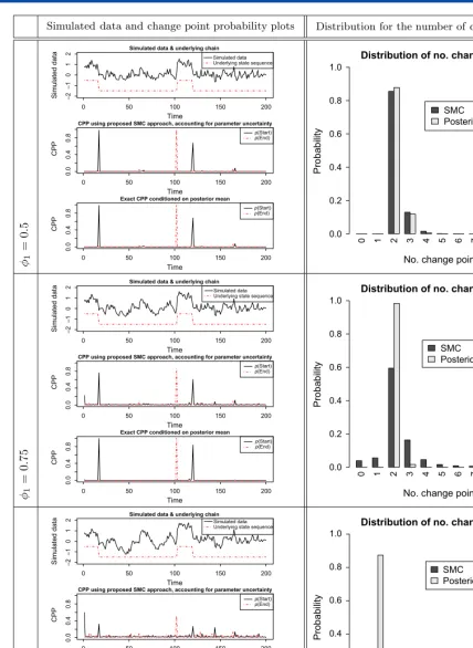
Figure 1 displays the various simulated time series and the state sequence of the underlying Markov chain in addition to plots for the change point probabilities (left column) and the distribution of the number of change points (right column) obtained via our proposed SMC based algorithm. The latent state sequence is common to all of the simulated time series and is denoted by the dashed line superimposed on the simulated time series plot.

Our change point results consider changes into and out of regime 1, which is that with smaller mean, for at least 2 time periods (k¼2 ands¼1 with an ordering constraint placed on the mean parameters). The change point probability (CPP) plots display the probability of switching into and out of this regime. In all simulated time series, there are two occurrences of this regime, starting at times of approximately 20 and 120, and ending at time 100 and continuing to the end of the data respectively.

In all three time series considered, our results indicate that our proposed methodology works well with good detection and estimation for the change point characteristics of interest. Change point probabilities are centred around the true locations of the starts and ends of the regime of interest with a degree of concentration dependent on the information contained in the data. The true number of regimes is the most probable in all three of the time series considered.

As/1increases, the distribution of the change point characteristics become more diffuse. This is what would be expected as the

data become less informative as/1increases. This uncertainty is a feature of the model, not a deficiency of the inferential method,

and it is important to account for it when performing estimation and prediction of related quantities. The proposed methodology is able to do this.

We also observe that the probability that there are no change points is not negligible for /1¼0.75 and for /1¼0.90. These

results illustrate the necessity of accounting for parameter uncertainty in change point characterization.

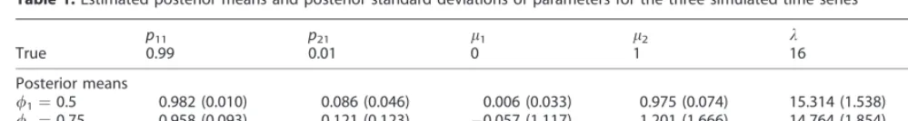
Table 1 displays the posterior means of the model parameter samples obtained via the SMC sampler. These are calculated by taking the weighted average of the weighted cloud of samples approximating the model parameter posterior distribution. In addition, we provide Monte Carlo estimates of the posterior standard deviation. We observe that the posterior values are reasonably close to the true values used to generate the time series. We note that as/1 increases and consequently the data

becomes less informative, less accurate estimates are provided with greater deviation from the true values and commensurate increase in standard deviation. Nevertheless, we observe that the model parameter posterior has been reasonably well approximated.

As a comparison, we also consider the exact change point distributions obtained by conditioning on these posterior means. We observe from the corresponding plots in Figure 1 that quite different results can be achieved. We observe that some of the uncertainty concerning the possible additional change points has been eliminated (see, e.g., the two CPP plots when/1¼0.75). In

addition, as illustrated by the righthand column of the figure, the distribution of the number of switches to the regime of interest has substantially more mass on two switches having occurred. This apparently improved confidence could be dangerously misleading in real applications.

The /1¼0.9 case in particular illustrates the importance of accounting for parameter uncertainty when considering change

points. We observe in the exact calculations that only one switch to the regime of interest is the most probable which occurs at the beginning of the data, and the second occurrence to the regime is generally not accounted for. The true behaviour of the underlying system is therefore not correctly identified in this instance. Thus obtaining results by conditioning on model parameters may provide misleading change point conclusions and accounting for model parameter uncertainty is able to provide a general overview with regards to different types of possible change point behaviours that may be occurring. In Bayesian inference one should, whenever possible, base all inference on the full posterior distribution, marginalizing out any nuisance variables and that is exactly what the proposed method allows us to do.

4.3. fMRI data

Functional magnetic resonance imaging allows the quantification of neuronal activityin-vivothrough the surrogate measurement of blood flow changes in the brain. The ability to measure these blood flow changes relates to the so-called BOLD (blood oxygenation level dependent) effect (Ogawa et al., 1990) where haemoglobin changes its magnetic properties dependent on whether it is carrying oxygen or not (oxyhaemoglobin and deoxyhaemoglobin are diamagnetic and paramagnetic respectively). By examining the small magnetic field changes, it is possible to quantify the relative changes in the oxygen concentrations in the blood, which are a downstream product of neuronal activation. More information regarding fMRI and its many inherent statistical problems can be found in Lindquist (2008).

As mentioned above, most analysis of fMRI experiments is conducted by assuming a postulated experimental design (see Worsley

et al., 2002 for example) and using standard linear modelling techniques, usually accounting for an AR component in the model.

The data analysed in this article comes from an anxiety inducing experiment. Next is the task description as given in Lindquistet al.

(2007):

Simulated data & underlying chain

Time

Simulated data

Simulated data Underlying state sequence

CPP using proposed SMC approach, accounting for parameter uncertainty

Time

CPP

p(Start)

p(End)

Exact CPP conditioned on posterior mean

Time

CPP

p(Start)

p(End)

0 1 2 3 4 5 6 7 8 9 ₁₀

SMC Posterior mean

Distribution of no. change points

No. change points

Probability 0.0 0.2 0.4 0.6 0.8 1.0

Simulated data & underlying chain

Time

Simulated data

Simulated data Underlying state sequence

CPP using proposed SMC approach, accounting for parameter uncertainty

Time

CPP

p(Start)

p(End)

Exact CPP conditioned on posterior mean

Time

CPP

p(Start)

p(End)

0 1 2 3 4 5 6 7 8 9 ₁₀

SMC Posterior mean

Distribution of no. change points

No. change points

Probability 0.0 0.2 0.4 0.6 0.8 1.0

Simulated data & underlying chain

Time

Simulated data

Simulated data Underlying state sequence

CPP using proposed SMC approach, accounting for parameter uncertainty

Time

CPP

p(Start)

p(End)

0 50 100 150 200

–2

–1

0

1

2

0 50 100 150 200

0.0

0.4

0.8

0 50 100 150 200

0.0

0.4

0.8

0 50 100 150 200

–2

–1

01

2

0 50 100 150 200

0.0

0.4

0.8

0 50 100 150 200

0.0

0.4

0.8

0 50 100 150 200

–2

–1

01

2

0 50 100 150 200

0.0

0.4

0.8

0 50 100 150 200

0.0

0.4

0.8

Exact CPP conditioned on posterior mean

Time

CPP

p(Start)

p(End)

0 1 2 3 4 5 6 7 8 9 ₁₀

SMC Posterior mean

Distribution of no. change points

No. change points

Probability 0.0 0.2 0.4 0.6 0.8 1.0

Figure 1.Results on simulated data generated from a Hamilton’s MS-AR(1) model. We consider a variety of data and display the change point probability plots and distribution of number of change points obtained by implementing our proposed sequential Monte Carlo based methodology. As a comparison, we also consider the exact change point distributions when conditioned on posterior means point estimates of the parameters

The design was an off-on-off design, with an anxiety-provoking speech preparation task occurring between lower-anxiety resting periods. Participants were informed that they were to be given two minutes to prepare a seven-minute speech, and that the topic would be revealed to them during scanning. They were told that after the scanning session, they would deliver the speech to a panel of expert judges, though there was ‘‘a small chance’’ that they would be randomly selected not to give the speech.

After the start of fMRI acquisition, participants viewed a fixation cross for 2 min (resting baseline). At the end of this period, participants viewed an instruction slide for 15 s that described the speech topic, which was to speak about ‘‘why you are a good friend’’. The slide instructed participants to be sure to prepare enough for the entire 7 min period. After 2 min of silent preparation, another instruction screen appeared (a relief instruction, 15 s duration) that informed participants that they would not have to give the speech. An additional 2 min period of resting baseline followed, which completed the functional run.

The time series were collected every 2 seconds for a total of 215 observations. The analysis in Lindquistet al.(2007) consisted of using an exponential weighted moving average (EWMA) approach which corrected for an AR error process to find a change point and to determine the duration of the change until a return to baseline had occurred. This methodology does not easily allow the incorporation of multiple change points and requires detrending of the data to be performed prior to the analysis. Using the methodology in this article, the detrending is added as another set of parameters to estimate within the SMC step providing a combined single step analysis, that is, the detrending within the model. This leads to an extension of Hamilton’s MS-AR(r) model which is defined as follows:

yt¼m0tbþlxtþat ð37Þ

at¼/1at1þ. . .;þ/ratrþt; tNð0;r2Þ: ð38Þ

Here,mtis ad·1 vector containing thedadditional exogenous covariates (detrending basis in this case) at timetassociated with the trend mean.b, ad·1 vector, comprising of the associated trend related coefficients. Note that the Hamilton’s MS-AR(r) model specified in (28) can be obtained by fixingb¼0. In addition, the presented method of this article allows the uncertainty in the estimation of the change points to be calculated. A 2-state Hamilton MS-AR(r) model with detrending can be used to model the considered time series (Peng, 2008), with the underlying state space beingXX¼ f‘resting’, ‘active’g.

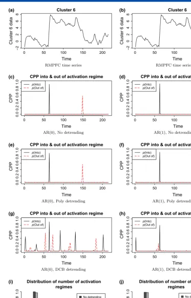
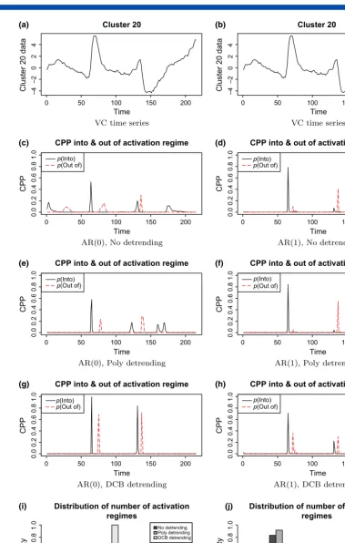
Several models and different detrending options are considered, mainly as an aid to discussion of the importance of taking care of time series properties in any fMRI analysis. First, as a baseline comparison, a model with independent errors (an AR(0) error process) and no detrending is used. This will show that this can be particularly unsatisfactory if a change point analysis is being used, which is unsurprising given that change point detection techniques are well known to breakdown in the presence of other forms of non-stationarity such as linear trends. The analysis then proceeds using various combinations of polynomial detrending (Worsleyet al., 2002) and discrete cosine basis detrending (Ashburneret al., 1999), along with an AR(1) error model. An AR(1) model for fMRI time series is probably the most commonly used and is the default in the Statistical Parametric Mapping (SPM) software (Ashburneret al., 1999). Two specific regions of the brain are of most interest. In the first, the time series comes from the rostral medial pre-frontal cortex (RMPFC), which is known to be associated with anxiety, while the second is from the visual cortex (VC) and shows activation associated with the task-related instructions (these are denoted (as in Lindquistet al.(2007)) as Cluster 6 and 20 respectively in the results plots and data set). The resulting change point distributions for the two regions of the brain can be seen in Figures 2 and 3 where we deem the region to be activated when there is a sustained changed for at least 5 time points in the region, thuss¼‘active’ andk¼5. The methodology in this article finds significant evidence, in terms of the number of change points, that there is at least one change point in both regions of the brain. This accords with the previous EWMA analysis, where both regions were shown to have a change point, with the RMPFC region associated with the anxiety stimulus.

In addition to the actual change point distributions, the HMM analysis allows for different models to be assessed and the effect of the models on the uncertainty regarding change points locations. For the RMFPC region, if an AR(0) with no detrending is used, then two distinct changes, one into the activation region and one out of the activation region are determined. However, if an AR(1) model is assumed, with or without polynomial detrending, the return to baseline is no longer clearly seen, and the series is consistent with only one change to activation from baseline during the scan. In this example, little difference is seen with the type of detrending, but considerable differences occur depending on whether independent errors are assumed or not. A little extra variation is found in the change point distribution if a discrete cosine basis is used, but this is likely due to identifiability issues between the cosine basis and the change points present.

Table 1.Estimated posterior means and posterior standard deviations of parameters for the three simulated time series

p11 p21 l1 l2 k /1

True 0.99 0.01 0 1 16 –

Posterior means

/1¼0.5 0.982 (0.010) 0.086 (0.046) 0.006 (0.033) 0.975 (0.074) 15.314 (1.538) 0.414 (0.073)

/1¼0.75 0.958 (0.093) 0.121 (0.123) 0.057 (1.117) 1.201 (1.666) 14.764 (1.854) 0.731 (0.086)

On examining the regions of the VC, the choice of detrending is critical. If a suitable detrending is assumed, in this case a discrete cosine basis within the estimation, a clear change point distribution with multiple change points is found. However, if no or a small order polynomial detrending is used, the change point distributions associated with the visual stimuli are masked. It is also noticeable that the assumption of an AR(1) error process increases the inherent variability in the change point distribution.

0 50 100 150 200 0 50 100 150 200

0 50 100 150 200 0 50 100 150 200

0 50 100 150 200 0 50 100 150 200

0 50 100 150 200 0 50 100 150 200

Cluster 6 (a) (b) (d) (c) (e) (f) (h) (g) (i) (j) Time

Cluster 6 data

RMPFC time series

Cluster 6

Time

Cluster 6 data

RMPFC time series

–2 02468 –2 02468 0.0 0.2 0.4 0.6 0.8 1.0 0.0 0.2 0.4 0.6 0.8 1.0 0.0 0.2 0.4 0.6 0.8 1.0 0.0 0.2 0.4 0.6 0.8 1.0 0.0 0.2 0.4 0.6 0.8 1.0 0.0 0.2 0.4 0.6 0.8 1.0 0.0 0.2 0.4 0.6 0.8 1.0 0.0 0.2 0.4 0.6 0.8 1.0

CPP into & out of activation regime

Time

CPP

p(Into)

p(Out of)

AR(0), No detrending

CPP into & out of activation regime

Time

CPP

p(Into)

p(Out of)

AR(1), No detrending

CPP into & out of activation regime

Time

CPP

p(Into)

p(Out of)

AR(0), Poly detrending

CPP into & out of activation regime

Time

CPP

p(Into)

p(Out of)

AR(1), Poly detrending

CPP into & out of activation regime

Time

CPP

p(Into)

p(Out of)

AR(0), DCB detrending

CPP into & out of activation regime

Time

CPP

p(Into)

p(Out of)

AR(1), DCB detrending

No detrending Poly detrending DCB detrending

No. activation regimes

Probability

AR(0), Distribution of number of regimes

0 1 2 3 4 5 6 7 8 9 0 1 2 3 4 5 6 7 8 9

No detrending Poly detrending DCB detrending

Distribution of number of activation regimes

Distribution of number of activation regimes

No. activation regimes

Probability

AR(1), Distribution of number of regimes

Figure 2.Change point analysis results for the RMPFC (Cluster 6) region of the brain with respect to different order of model and detrending

We also considered an AR(1) error process with/1¼0.2 under all types of detrending. Fixing the AR parameter to this value is a

common analysis approach, as featured in the SPM software. The change point results (not presented) contained features present in both results AR(0) and AR(1) analysis with more peaked and centred change point probability features compared to the presented AR(1) results, due to accounting for less uncertainty with respect to fixing/1¼0.2.

Cluster 20 (a) (b) (c) (d) (e) (f) (g) (h) (i) (j) Time

Cluster 20 data

VC time series

Cluster 20

Time

Cluster 20 data

VC time series

CPP into & out of activation regime

Time

CPP

p(Into)

p(Out of)

AR(0), No detrending

CPP into & out of activation regime

Time

CPP

p(Into)

p(Out of)

AR(1), No detrending

CPP into & out of activation regime

Time

CPP

p(Into)

p(Out of)

AR(0), Poly detrending

CPP into & out of activation regime

Time

CPP

p(Into)

p(Out of)

AR(1), Poly detrending

CPP into & out of activation regime

Time

CPP

p(Into)

p(Out of)

AR(0), DCB detrending

CPP into & out of activation regime

Time

CPP

p(Into)

p(Out of)

AR(1), DCB detrending

No detrending Poly detrending DCB detrending

No. activation regimes

Probability

AR(0), Distribution of number of regimes

No detrending Poly detrending DCB detrending

Distribution of number of activation regimes

Distribution of number of activation regimes

No. activation regimes

Probability

0 50 100 150 200

–4 –2 0 2 4 0.0 0 .2 0.4 0 .6 0.8 1 .0 0.0 0 .2 0.4 0 .6 0.8 1 .0 0.0 0 .2 0.4 0 .6 0.8 1 .0 0.0 0 .2 0.4 0 .6 0.8 1 .0 0.0 0 .2 0.4 0 .6 0.8 1 .0 0.0 0 .2 0.4 0 .6 0.8 1 .0 0.0 0 .2 0.4 0 .6 0.8 1 .0 0.0 0 .2 0.4 0 .6 0.8 1 .0

0 1 2 3 4 5 0 1 2 3 4 5

AR(1), Distribution of number of regimes

0 50 100 150 200

0 50 100 150 200 0 50 100 150 200

0 50 100 150 200 0 50 100 150 200

0 50 100 150 200 0 50 100 150 200

–4

–2

0

2

4