Methodologies for predicting natural frequency variation of a suspension bridge

Original citation:

Laory, Irwanda, Trinh, Thanh N., Smith, Ian F.C. and Brownjohn, James M.W.. (2014) Methodologies for predicting natural frequency variation of a suspension bridge. Engineering Structures, Volume 80 . pp. 211-221.

Permanent WRAP URL:

http://wrap.warwick.ac.uk/66480

Copyright and reuse:

The Warwick Research Archive Portal (WRAP) makes this work by researchers of the University of Warwick available open access under the following conditions. Copyright © and all moral rights to the version of the paper presented here belong to the individual author(s) and/or other copyright owners. To the extent reasonable and practicable the material made available in WRAP has been checked for eligibility before being made available.

Copies of full items can be used for personal research or study, educational, or not-for-profit purposes without prior permission or charge. Provided that the authors, title and full bibliographic details are credited, a hyperlink and/or URL is given for the original metadata page and the content is not changed in any way.

Publisher’s statement:

© 2014, Elsevier. Licensed under the Creative Commons Attribution-NonCommercial-NoDerivatives 4.0 International http://creativecommons.org/licenses/by-nc-nd/4.0/

A note on versions:

The version presented here may differ from the published version or, version of record, if you wish to cite this item you are advised to consult the publisher’s version. Please see the ‘permanent WRAP URL’ above for details on accessing the published version and note that access may require a subscription.

Methodologies for predicting natural frequency variation of a suspension

1

bridge

2

Irwanda Laory1, Thanh N. Trinh2, Ian F. C. Smith2 and James M. W. Brownjohn3 3

1_{School of Engineering, University of Warwick, Coventry, United Kingdom} 4

Email: [email protected]

5

2_{Applied Applied Computing and Mechanic Laboratory, Swiss Federal Institute of} 6

Technology Lausanne (EPFL), Lausanne, Switzerland

7

3_{Vibration Engineering Section, College of Engineering, Mathematics and Physical Sciences,} 8

The University of Exeter, Exeter, United Kingdom

9 10 11

Abstract

12

In vibration-based structural health monitoring, changes in the natural frequency of a structure 13

are used to identify changes in the structural conditions due to damage and deterioration. 14

However, natural frequency values also vary with changes in environmental factors such as 15

temperature and wind. Therefore, it is important to differentiate between the effects due to 16

environmental variations and those resulting from structural damage. In this paper, this task is 17

accomplished by predicting the natural frequency of a structure using measurements of 18

environmental conditions. Five methodologies - multiple linear regression, artificial neural 19

networks, support vector regression, regression tree and random forest - are implemented to 20

predict the natural frequencies of the Tamar Suspension Bridge (UK) using measurements 21

taken from three years of continuous monitoring. The effects of environmental factors and 22

traffic loading on natural frequencies are also evaluated by measuring the relative importance 23

of input variables in regression analysis. Results show that support vector regression and 24

random forest are the most suitable methods for predicting variations in natural frequencies. 25

In addition, traffic loading and temperature are found to be two important parameters that 26

need to be measured. Results show potential for application to continuously monitored 27

structures that have complex relationships between natural frequencies and parameters such as 28

KEY WORDS:Environmental effect, artificial neural network, support vector regression,

30

regression tree, random forest, variable importance, suspension bridge.

31

32

1. Introduction

33

Many vibration-based approaches in structural health monitoring have been designed to 34

identify changes in natural frequency values for the purpose of detecting changes in structural 35

conditions that may indicate structural damage and degradation. In reality, however, civil 36

engineering structures are subject to environment and operating effects caused by changes in 37

temperature, traffic, wind, humidity and solar-radiation [1-5]. Such environmental effects also 38

change natural frequency values, hence concealing changes due to structural damage [6-10]. 39

Therefore, it is important to distinguish between changes due to structural damage and 40

changes resulting from environmental effects. This task is managed observing then modeling 41

dependencies of natural frequencies on environmental parameters [11]. The prediction of 42

natural frequencies of structures under environmental changes has been studied using methods 43

such as linear regression analysis, artificial neural networks and support vector regression. 44

Multiple linear regression (MLR) was employed to predict changes in natural 45

frequencies of the Alamosa Canyon Bridge (USA) due to environmental temperature variation 46

[9] with natural frequencies formulated as a linear function of temperature data. It was found 47

that the changes in the frequencies were linearly correlated with temperature taken from 48

different locations on the bridge. Peeters et al. [12] conducted a one-year monitoring study for 49

the Z24-Bridge (Switzerland) before it was deliberately damaged, applying a linear regression 50

analysis to distinguish normal frequency changes from abnormal changes due to damage. 51

Also, for this concrete box girder bridge, Peeters and Roeck [13] applied an autoregressive 52

method with exogeneous inputs (ARX) to predict the bridge natural frequencies, where no 53

Dewolf [3] simulated the varying natural frequencies under temperature changes using a 55

linear regression analysis, concluding that the long-term variations of natural frequencies are 56

closely related to the variation in in-situ concrete temperature for the three frequencies they 57

measured. The MLR method has also been used to predict natural frequencies of suspension 58

bridges and a footbridge using long-term monitoring data [11, 14]. 59

Artificial neural networks (ANNs) have been successfully applied in fields such as 60

pattern recognition [15], artificial intelligence [16] and civil engineering [17-20]. For long-61

term monitoring of structures, ANNs have been employed to predict time-dependent natural 62

frequencies of a structure in order to eliminate the environmental effects on vibration-based 63

damage detection procedures. For example, Ni et al. [21] applied an ANN to formulate the 64

correlation between the natural frequencies and environmental temperatures taken from the 65

cable-stayed Ting Kau Bridge (Hong Kong). Zhou et al [22] further investigated the 66

performance of the ANNs formulated using the early stopping technique by constructing 67

three different kinds of input, including mean temperatures, effective temperatures and 68

principle components (PCs) of temperatures. The results indicated that when a sufficient 69

number of PCs were taken into account, the ANN using temperature PCs as inputs predicted 70

natural frequencies more accurately than that when using the mean temperatures. More 71

studies on ANNs for the prediction of structural responses are found in references [22-25]. 72

Support vector regression (SVR) is an application form of support vector machines that 73

is a learning system using a high dimension feature space [26-27]. An attractive characteristic 74

of SVR is that instead of minimizing the observed training error such as with MLR and 75

ANNs, SVR involves minimizing the generalized error bound in order to achieve good 76

performance. The generalized error bound is the combination of the training error and a 77

regularization term that controls the complexity of prediction functions. A good overview of 78

categorization and pattern recognition as well as structural health monitoring [27, 30]. Ni et 80

al. [31] applied SVR to predict natural frequencies of the cable-stayed Ting Kau Bridge 81

(Hong Kong) subjected to temperature variations taken from one-year measurement data, the 82

method exhibiting better prediction capability than the MLR method. Also using 83

measurement data of this bridge, Hua et al. [32] combined principle component analysis 84

(PCA) and SVR to simulate temperature-frequency correlations. It was found that the SVR 85

method trained using the PCs of measured temperature data outperformed that trained using 86

measured temperature data directly. 87

The methodologies used above are based on parametric functions that specify the form 88

of the relationship between inputs and a response (output) but in many cases, the form of the 89

relationship is unknown. Regression tree (R_Tree) methods offer a non-parametric 90

alternative [33] that has been used extensively in a variety of fields. The method has been 91

found to be especially useful in biomedical and genetic research, speech recognition and other 92

applied sciences [34]. Recent studies in the machine-learning field found that significant 93

improvements in prediction accuracy have resulted from growing an ensemble of trees in a 94

random way, a methodology called random forest (RF)[35]. It has been demonstrated that RF

95

has improved prediction accuracy in comparison to other regression methods [36] but 96

additionally provides measures of variable importance for each input variable [37-38]. This 97

method has not been evaluated for its applicability to structural health monitoring, so this 98

paper investigates the performance of RF on predicting natural frequencies through a case 99

study of a suspension bridge. 100

The studies mentioned above have proposed methodologies for predicting the dynamic 101

responses of bridges, but none has compared methodologies for prediction accuracy. This 102

paper compares five methodologies – multiple linear regression, artificial neural networks, 103

predict natural frequencies of a suspension bridge. Confidence intervals are then defined for 105

the best method to differentiate the effects due to environmental changes from those caused 106

by structural damage. Furthermore, the individual effects of temperature, wind and traffic 107

loading on the natural frequency responses of the bridge are evaluated using the variable 108

importance metric in regression analysis. 109

2. Methodologies for predicting natural frequencies of the bridge

110

2.1. Multiple linear regression (MLR)

111

Assuming that a response variable y (for example natural frequency) is linearly related 112

to the p input variables (for example temperature, wind and traffic loading) x₁,...x_p so that 113

0 1

p

i i

i

y   x e



 



114

This relationship is known as a linear regression analysis, where _i is the regression 115

coefficient associated with the th

i input variable x_i and e the random error with mean zero 116

and variance 2

. Using the dataset of n observations in measurement time series, the 117

unknown coefficients _i are determined using the least-squares method. 118

2.2. Artificial neural networks (ANNs)

119

Artificial neural networks can be used as a nonlinear regression method to predict the 120

natural frequency of a bridge. ANN is a two-stage regression in which the first stage is to 121

create derived features Z_m, represented by hidden layer, from linear combinations of the 122

inputs and the second stage is to model the output Y_m as a function of linear combinations of 123





 

0 0

, 1,..., ,

, 1,..., ,

, 1,..., ,

T

m m m

T

k k k

k k

Z X m M

T Z k K

f X T e k K

  

 

  

  

  

(2)

125

where Z





sigmoid ( ) 1/ (1v  ev), e the random error, _i and _i are unknown parameters. Given a 127

training set









unknowns so that the sum-of-squared errors as a measure of fit reaches a minimum value. 129







 



,

K N

ik k i

k i

R   y f x

 





130

The generic approach to minimizing, R

 

propagation. A two-layer back-propagation neural network (BPNN) is employed to predict 132

the natural frequencies of a structure. BPNN is first trained using the training set in order to 133

formulate the relationship between the natural frequencies and environmental factors 134

including direct loading such as traffic. BPNN is composed of one hidden layer and one 135

output layer with a tan-sigmoid transfer function in the hidden layer and a linear transfer 136

function in the output layer. The tan-sigmoid transfer function is capable of capturing the 137

nonlinear relationship between input variables (in our example three of them) and output 138

variables (in our example individual natural frequencies). 139

An important parameter to be determined when using BPNN for prediction tasks is the 140

optimal number of hidden nodes in the hidden layer. A network with too few hidden nodes 141

might not have enough flexibility to capture the nonlinearities in the relationship while a 142

2.3. Support vector regression (SVR)

144

The strategy of SVR is to transform nonlinear relationships from the original space into 145

linear relationships in a new space (or feature space) defined using a kernel function so as to 146

discover relationships more easily [27, 36]. The linear function in the new space is given by 147

 

 

y x w  x  b e (4)

148

where w is the weight vector; b is the bias constant and 

 

transfers the input vector x into the new space. Given a training set









SVR model is obtained by minimizing the following objective function [39] 151





 

2 , ,

1

1 1

min ,

2 2

subject to , 1,..., .

N T

i w b e

i

T

i i i

J w e w w e

y w x b e i N







 

   



(5)

152

where  is the regularization parameter and e_i is the error. Such optimization that is subject 153

to a condition is solved using the Lagrangian function 154











 



1

, , , ,

N

T

i i i i

i

L w b e J w e  w  x b e y



 



155

 

 

0 , 1,..., .

0 0, 1,..., .

N i i i N i i i i T

i i i

L w x w L b L

e i N

e

L

w x b e y i N

           _{  }     _{  }     _{   }       _{      }  





Elimination of w and e yields a set of linear equations that are written in the matrix form 158 1 0 0 1 1 T N N N b Y I        _  _{ }         

  (8)

159

where Y 













and  is a NN kernel matrix defined by a kernel function as 161

 

 





ij  xi  xj K x xi j

   . (9)

162

The kernel function is designed to compute inner-products in the new space using only the 163

original input data. The choice of K implicitly determines  and the new space. Thus, the 164

advantage of kernel functions is that if a kernel function K is given, it is not necessary to 165

know the explicit form of the mapping function 

 

generally depends on the application domain. It has been shown that Gaussian radial-basis 167

function (RBF) is a reasonable first choice of kernel functions since it has only a single 168

parameter (standard deviation,  ) to be determined [27, 40]. The Gaussian RBF is expressed

169





2

, xi xj

i j

K x x e   . (10)

171

Solving Equation (8) identifies the values of  and b. Then, substituting these values into 172

Equation (4) leads to the prediction 173

 





1

,

N

i i

i

y x K x x b







174

There are only two tuning parameters,  and  , that need to be determined when using the

175

RBF kernel function and their optimal values are determined using the grid search method . 176

Possible intervals for the two parameters are first defined. Then all grid points are tried to find 177

the one giving the best accuracy. For each combination of the two parameters, SVR is trained 178

using the training data and their performance is evaluated by a ten-fold cross-validation 179

scheme. 180

2.4. Regression tree (R_Tree)

181

Regression tree is a nonparametric statistical method [33] that offers an alternative to 182

parametric regression methods which usually require assumptions and simplifications to form 183

the relationship. A regression tree is built by recursively partitioning the entire dataset, 184

represented by a root node, into more homogeneous groups with each to be represented by a

185

node. When the splitting process terminates, each resulting group is referred to as a terminal 186

node. Splitting at each node is based on one value of an input variable that leads to the most 187

homogeneous resulting nodes. Assuming that we have a partition into M regions R₁, R₂, ..., 188

M

R the system model is identified as 189

( ) ( _{j j m})

y x ave y x R e (11)

Where y_j and x_j represent the response and input variables at jth observation respectively. 191

Equation 10 shows that the predicted response is the average of y_j in region R_m with the 192

errore. 193

A simple regression tree is built with two input variables x₁ and x₂ and a response y

194

by considering a recursive partition as shown in Figure 1(a). First, we select the splitting

195

variable (for example, x₁) and the split point (for example s₁) in order to achieve the most 196

homogeneous splitting groups and split the space of the dataset into two groups. The selected 197

variable and point solve 198

1 2

2 2

1 2

,

( , ) ( , )

min ( ) ( )

i i

i i

j s

x R j s x R j s

y c y c

 

 

   

 







199

1

c and c₂ are the mean value of all the responses in the corresponding groups. Then, each of 200

these groups is further split into two more groups. As shown in Figure 1(a), the group x₁s₁

201

is split at x₂ s₂ and finally the group x₁ s₁ is split at x₁ s₃. The process results in four 202

groups R₁, …, R₄. This process can be represented by the binary tree (Figure 1(b)). The 203

entire dataset sits at the top of the tree, as a so-called root node. Observations (data points) 204

satisfying the condition at each node are assigned to the left branch, and the others to the right 205

branch. The terminal nodes of the tree correspond to the groups, R₁, .., R₄. Once a tree has 206

been built, the response for any new observation can be predicted by following the path from 207

the root node down to the appropriate terminal node of the tree, based on the observed values 208

of the splitting variables. 209

When determining tree size, note that a small tree may not capture a nonlinear 210

relationship that may exist while a very large tree may over-fit the data. Therefore, tree size is 211

preferred strategy is to gradually increase the tree size and evaluate the accuracy of each tree 213

size until each node contains fewer than a given number of observations (for example, 5). 214

Then this large tree is pruned by sequentially cutting off branches that add the smallest 215

capability to predictive performance of the tree according to a specified pruning criterion. 216

2.5. Random forest (RF)

217

A random forest is a combination of regression trees that are grown in random ways 218

[35]. The idea behind the random forest method is to generate an ensemble of low-correlated 219

regression trees and average results in order to reduce variance. The low-correlated trees are 220

generated by adding randomization in two steps: (i) each tree is grown using a random sub-221

dataset of observations and (ii) each node of a tree is split using a random subset of input 222

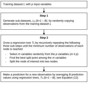
variables. Figure 2 shows the layout of the random forest method. 223

The first step is to generate B sub-datasets of observations by randomly copying 224

observations from the original training set L until each sub-dataset has the same number of

225

observations N as the original training set. Some observations can be chosen several times

226

for each sub-dataset, whereas others are not chosen at all. It has been proved that about 37% 227

of the observations in the original training set are not chosen for each sub-dataset [38, 41]. 228

The collection of non-chosen observations corresponding to each sub-dataset functions as a 229

validation set. Each sub-dataset is denoted L_b where b1, 2,...,B. 230

The second step involves growing a regression tree

 

 

step is to reduce further the correlation between the regression trees that enter into the 232

averaging step later. This is achieved during the tree-growing process by randomly selecting 233

a subset of m input variables from all p input variables





A regression tree is grown by recursively repeating the following three sub-steps for each 235

- Randomly select a subset of m variables from all p variables. 237

- Find the best split among the m variables. 238

- Split the selected node into two resulting nodes. 239

After B regression trees are grown from B sub-datasets, an ensemble of these B trees 240

is called a random forest. The random forest makes a prediction for a new observation x by

241

using each regression tree T_b in the forest to obtain a prediction y_b

 

242

prediction values from the B trees: 243

 

 

1

1 B

b b

y x y x e

B 





244

3. Case study subject: The Tamar suspension bridge

245

The Tamar Suspension Bridge, as shown in Figure 3, is a road bridge connecting 246

Saltash to Plymouth in southwest England. The original bridge was designed as a 247

conventional suspension bridge with symmetrical geometry and was first opened in 1961. The 248

total length is 642 m with a main span of 335 m and side spans of 114 m and the tower height 249

is 73 m. Trusses are 4.9 m deep with chords of welded hollow box structures. To meet the 250

requirement that bridges should be capable of carrying lorries up to 40 tons, the Tamar Bridge 251

was strengthened and widened in March 1999 and the upgrading was completed in December 252

2001[42-43]. The upgrading included replacing the original composite main deck by a three-253

lane orthotropic steel deck, adding single lane cantilevers at each side of the truss and 254

installing sixteen new cables acting as additional stays to carry the additional dead load of 255

new cantilever lanes and associated temporary works. Figure 4 shows the layout of one of the 256

truss sections with the main orthotropic deck and two cantilever lanes. 257

Many types of sensors were installed during and subsequent to the strengthening and 258

displacement sensors, thermometers, load cells and accelerometers. Most recently, a robotic 260

total station was added to monitor the deflection of the bridge deck and a pair of 261

extensometers installed to track relative movement across the single expansion joint located 262

around the Saltash Tower [45]. Measurement data have been collected continuously since 263

February 2007. 264

These data used in this study include air temperature, wind velocity, the measured 265

natural frequencies of the bridge and the number of vehicles crossing the bridge every hour. 266

Vehicle crossing data were available from the bridge toll reports, temperature and wind values 267

are 30-minute averages of data sampled at either 1Hz from four thermistors on the cable and 268

deck and an anemometer close to midspan, while frequencies are derived from modal analysis 269

of 64-Hz sampled acceleration signals from a pair of accelerometers located near mid span. 270

Locations of these sensors are shown in Figure 5. The covariance-driven stochastic subspace 271

identification (SSI-COV) procedure operated automatically on the acceleration data after 8-272

fold decimation, reporting frequency and damping estimates at 30 minute intervals. 273

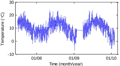
Figure 6 shows the time history of air temperature for three years, including daily and 274

seasonal temperature variations. The temperature ranges from -5 °C to 25 °C between winter 275

and summer. The first five natural frequencies of the bridge are summarized in Table 1. 276

4. Results

277

The five regression methodologies presented in the previous section are applied to 278

predict the natural frequency variation of the Tamar Bridge based on environmental factors as 279

well as traffic loading. The prediction is performed for each natural frequency separately. The 280

measurement data taken from July 2007 to January 2010 on the Tamar Bridge are divided into 281

two non-overlapping and independent data sets: a training set of 70% and a test set of 30%. 282

natural frequencies, the test set is used for assessing prediction accuracy (from June 2009 to 284

January 2010). 285

4.1. Multiple linear regression

286

The relationship between natural frequency responses and air temperature, wind and 287

traffic loading are first formulated for each frequency using the least square method. Figure 7 288

shows the prediction of the 10-day time histories (from 20 to 30 July 2009) of the third 289

frequency that is compared with the measured frequency in the test phase. This figure 290

indicates that the predicted frequency is unable to capture the high variation in the natural 291

frequency. Table 2 presents the mean square error (MSE) values in the training and test sets, 292

where the error is the difference between the measured frequency value and its corresponding 293

predicted value. For frequency 1 and 3, MSE values in the training set are somewhat larger 294

than those in the test set. This is because there are more outliers in the training data than in 295

the test set. 296

4.2. Artificial neural networks

297

The optimal number of hidden nodes in the hidden layer is determined so that the 298

validation error reaches the minimum value. To do this, a set of neural networks with respect 299

to the increasing number of hidden nodes from 1 to 50 are trained using training data. The 300

number of hidden nodes of the neural network that gives the minimum error is taken as the 301

optimal number. 302

Table 3 presents the optimal numbers of hidden nodes for five natural frequencies, 303

together with MSE values of the training set and the test set. The optimal number of hidden 304

nodes for five frequencies ranges from 10 to 33 nodes. These values are close to the optimal 305

value (19 hidden nodes) for the first natural frequency of the Ting Kau cable-stayed bridge 306

[46]. Figure 8 shows the predicted natural frequency along with the measured frequency. 307

prediction value than multiple linear regression. Comparing the prediction capability of ANN 309

with other methods is further discussed in Section 4.6. 310

4.3. Support vector regression

311

Table 4 presents the optimal values of  and  that give the best performance (lowest 312

MSE) of SVR for five natural frequencies. The corresponding MSEs are also listed in this 313

table. Comparing the MSE values in Table 4 with Table 2 and Table 3 indicates that the SVR 314

method has a better performance than the MLR and ANN methods in both the training set and 315

the test set. For example, the prediction error (in the test set) for frequency 5 using SVR is 316

reduced by 20% when compared with the prediction error using MLR. Figure 9 shows the 317

predicted and measured time histories of frequency 3 from July 20 to 30, 2009. It is shown 318

that the predicted frequencies closely match the measured ones. 319

4.4. Regression tree

320

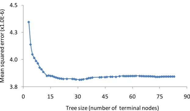
Figure 10 shows the mean squared error with respect to the increasing number of 321

terminal nodes (i.e. tree size) of the pruned tree for the first natural frequency. The optimal 322

tree size (i.e. the point where increasing tree size only leads to minor decrease of MSE) for 323

this frequency is composed of 31 terminal nodes. The optimal tree sizes for the second and 324

third frequencies are 44 and 35 terminal nodes respectively (Table 5). It is observed that the 325

higher frequency requires more terminal nodes, leading to a larger tree size, i.e. higher tree 326

complexity. Table 5 also presents the mean squared errors in the training and test sets. The 327

prediction of the R_Tree method is better than that of the ANN and MLR methods but it is not 328

as good as that of the SVR method. 329

Figure 11 shows the 10-day time histories of measured and predicted frequencies from 330

July 20 to July 30, 2009. For both sets, the predicted frequency time history reasonably 331

is because the observations at the peaks fall into the same groups where the predicted 333

responses are equal to the mean of measured responses within the corresponding group. 334

4.5. Random forest

335

When applying the random forest method for regression analysis, three parameters need 336

to be determined: (i) the sufficient number B of trees, (ii) the optimal number of observations 337

in each terminal node and (iii) the number m of input variables randomly chosen as 338

candidates for splitting at each node. For the Tamar Bridge, there are three input variables (i.e. 339

3

p ) including temperature, wind and traffic. For this case study, to reduce the correlation 340

between regression tress, the number of input variables chosen for splitting at each node is 2 341

(i.e. m2). 342

Figure 12 shows that when the number of trees increases, the mean squared error 343

computed from the validation set decreases. The prediction is stable at about 100 trees for 344

both cases of 1 and 50 observations in each terminal node. It is seen that the tree with 50 345

observations in terminal nodes performs better than that with only one observation in terminal 346

nodes. This is attributable to the over-fitting situation when growing a tree to its maximum 347

size (i.e. one observation in terminal nodes). 348

Figure 13 shows the change in the normalised mean squared error with respect to the 349

increase in the number of observations in terminal nodes for 5 frequencies. For each 350

frequency, the normalised MSE is calculated by dividing the MSE by the difference between 351

maximum and minimum MSE. When the number of observations in terminal nodes starts 352

increasing, initially the normalised MSE of all five frequencies drops dramatically to a 353

minimum and then it increases gradually. The optimal number of observations in terminal 354

nodes ranges from 10 to 50 observations. Table 6 presents the optimal number of 355

observations for each frequency together with its mean squared errors computed from the 356

errors as compared with those from the previous four methods. Figure 14 compares the 358

predicted natural frequency with the measured frequency. The predicted frequency closely 359

matches the measured one. 360

4.6. Performance comparisons and discussions

361

In order to find a suitable method to predict the natural frequency responses from 362

environmental measurement data for a suspension bridge, the prediction capability of five 363

regression methods are compared. The result of a regression method can have a very good fit 364

to the training data; however, it may poorly predict the response for a new observation. Thus, 365

the prediction capability of these methods is evaluated through prediction error that is defined 366

as the mean squared error from the test set, with a smaller prediction error indicating a better 367

prediction capability. When comparing the prediction error of the five regression methods 368

from Table 2 to Table 6, it can be seen that the four nonlinear regression methods (ANNs, 369

SVR, R_Tree and RF) predict frequencies more accurately than the MLR method. Table 7 370

presents the reduction in the prediction error for these methods when using the prediction 371

error of the MLR method as a basis. For frequency 5, SVR and RF can reduce the prediction 372

error up to 20% when compared with MLR. The good performances of SVR and RF indicate 373

the possibility of existence of non-linear correlations between natural frequency responses and 374

environmental factors as well as traffic loading for the Tamar Suspension Bridge. In addition, 375

comparing Figure 11 and Figure 14 demonstrates that RF employing multiple trees, which are 376

grown in a random way, can lead to better predictions than the R_Tree method that employs a 377

single tree. RF is able to capture the high variations at peaks of frequency time histories. 378

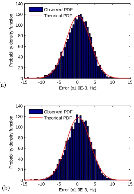
The performance of SVR and RF are further assessed through a normality test [47]. 379

From a statistical point of view the error, which is the difference between the predicted value 380

and the corresponding measured frequency value, complies with a normal distribution with 381

with the corresponding theoretical curves of the normal distribution obtained using the mean 383

and standard deviation values computed from error values. The figure shows the observed 384

probability distribution of the error for SVR and RF methods is in good agreement with a 385

normal distribution with zero mean. 386

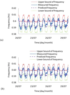
SVR and RF are used to define the confidence intervals around the predicted natural 387

frequencies for a new observation. It is found that the error in the training data for SVR and 388

RF also have a normal distribution with zero mean. Thus, the confidence interval is defined 389

based on the error variance of the training data. Figure 16 shows the identified and predicted 390

natural frequencies for RF between July 20 and July 30 (2009), together with the 95% 391

confidence interval for the second natural frequency. For the test set, the ratio of the data that 392

falls within the 95% confidence level to the full set of the data is referred to as the success 393

rate. For SVR, the success rates for frequencies 1 to 5 are 98%, 91%, 98%, 94% and 91%, 394

respectively. The corresponding success rates for RF are 98%, 91%, 98%, 94% and 89%. 395

These high success rates indicate that the variations in bridge natural frequencies can be 396

accounted for by measuring temperature, wind and traffic loading. These rates also 397

demonstrate the consistency of continuously monitored data from 2007 to 2010, thereby 398

establishing a baseline data for continuous health monitoring of the bridge. In addition, the 399

success rate can be used as a damage-detection index. If the success rates for future natural 400

frequencies change, it is likely that the bridge has experienced some kind of structural change. 401

5. Effects of environmental factors and traffic loading on natural frequencies of the

402

bridge

403

The changes in bridge natural frequencies are adequately accounted for by three factors: 404

temperature, wind and traffic loading. This study identifies the degree to which each factor 405

has an effect on the frequency change. Simultaneous effects of these factors on the first five 406

importance of input variables in regression analysis. The measure of relative importance 408

indicates the variables that are highly related to the response for interpretation purposes. 409

5.1. Evaluation of effects using relative importance metrics of the multiple linear regression

410

method

411

Multiple linear regression can be used to evaluate the contribution of an individual input 412

variable x_j





compared with that of other variables using a metric of so-called relative importance. Several 414

relative importance metrics have been proposed to assess the amount of variation in the 415

response that is explained by each individual variable [48-49]. In this study, since the 416

correlation between input variables is negligible, the relative importance of each individual 417

variable is defined as the squared correlation coefficient of an input variable x_j with the 418

response y. 419

Figure 17 shows the relative importance of temperature, wind and traffic loading using 420

MLR for the first five natural frequencies of the bridge. The effects of temperature, wind and 421

traffic loading on the first frequency are 8%, 18% and 74%. Such effects correspond to 34%, 422

10% and 56% for the second frequency. They are 28%, 10% and 62% for the third frequency 423

and 22%, 10% and 68% for the fifth frequency. Except for the fourth frequency (i.e. 70%, 424

21% and 9%), based on relative importance metrics defined using MLR, traffic loading is the 425

main factor that affects the natural frequencies. 426

5.2. Evaluation of effects using relative importance metrics of the random forest method

427

The random forest method has improved the prediction accuracy in comparison to other 428

prediction methods. Besides, RF also evaluates the relative importance of variables in a 429

dataset in order to measure the prediction strength of each variable. 430

chosen observations (about 37%) are utilized as validation observations for that tree. The 433

computation of the importance of an input variable x_j is carried out one tree at a time. First, 434

when the bth tree T_b is grown, the validation observations are then used to determine the mean 435

squared error from the validation data MSE_b. Next, the values of variable x_j in the validation 436

data are randomly permutated while leaving the values of all other variables unchanged. Then, 437

the permuted observations are used in the tree T_b and the mean squared error from the 438

permuted validation data MSE_b

 

values will reduce the prediction accuracy of each observed value in the validation data. Thus, 440

 

b j

MSE x from the permuted validation data is larger than MSE_b from the un-permuted 441

data. 442

Finally, a measure of the importance of the jth variable x_j is obtained by averaging the 443

mean squared errors from the permuted validation data over all of the trees: 444

 



 



1

1 B

j b j b

b

imp x MSE x MSE

B 





445

The relative importance of each variable is computed by normalizing its importance to 446

the summation of the importance of all variables. The relative importance metrics are 447

expressed in percentage. Figure 18 shows the relative importance of temperature, wind and 448

traffic loading on the natural frequency responses of the bridge. There is a significant effect 449

of traffic loading on the frequency. Figure 18 also indicates that while the effect of traffic 450

loading decreases from frequencies 1 to 5, the effect of temperature increases respectively. 451

Both effects are almost similar for frequency 5 and the effect of temperature is more dominant 452

5.3. Discussion

454

Comparing Figure 17 and Figure 18 shows that although variable importance metrics 455

are defined in two different ways using multiple linear regression and random forest, the 456

importance rankings for temperature, wind and traffic are identical. For the first frequencies, 457

the averaged percentages of the effects taken from both variable importance metrics are about 458

8%, 17% and 75% respectively. Such percentages correspond to 26%, 15% and 59% for the 459

second frequency, 24%, 9% and 66% for the third frequency, 60%, 22% and 18% for the 460

fourth frequency and 31%, 11% and 58% for the fifth frequency. A possible reason for the 461

effect of traffic loading is that there is a significant contribution of the traffic mass to the total 462

mass of the truss-span suspension bridge. Despite the strong influence on other frequencies, 463

the relative effect of the traffic on the fourth frequency is quite small. This could be due to the 464

fact that the fourth frequency refers to a torsional vibration mode while other frequencies refer 465

to vertical and lateral modes. 466

As for temperature effects, the influence on the variation of the fourth and fifth 467

frequencies is larger than that of the other frequencies. This could be caused by the non-linear 468

temperature distribution due to solar radiation. In general, for successful data interpretation 469

when monitoring natural frequency responses of suspension bridges, the effects of both traffic 470

loading and temperature need to be taken into account. 471

6. Conclusions

472

This paper compares five methodologies to predict the natural frequency responses of a 473

suspension bridge using measurements of temperature, wind and traffic loading. The 474

following conclusions are drawn 475

 Random forest and support vector regression are the most appropriate methods for

476

predicting the natural frequencies of a suspension bridge using measurement data of 477

 The relative importance of input variables of regression analysis is a useful metric to 479

evaluate the simultaneous effects of environmental factors and traffic loading on the 480

long-term natural frequency responses of a bridge. 481

 Traffic loading and temperature are the most influential parameters on natural frequencies

482

of the suspension bridge studied. Obtaining these parameters should be a priority when 483

using natural frequency changes to detect damage. 484

Acknowledgements

485

The authors are grateful to Dr. Minh-Hai Pham and Dr. Ki-Young Koo for their contributions 486

to this research. 487

References

488

[1] Wahab MA, De Roeck G. Effect of temperature on dynamic system parameters of a highway

489

bridge. Structural Engineering International. 1997;7:266-70.

490

[2] Yuen K-V, Kuok S-C. Ambient interference in long-term monitoring of buildings. Engineering

491

Structures. 2010.

492

[3] Liu C, DeWolf JT. Effect of temperature on modal variability of a curved concrete bridge under

493

ambient loads. Journal of Structural Engineering. 2007;133:1742-51.

494

[4] Xu Z-D, Zhishen Wu. Simulation of the effect of temperature variation on damage detection in a

495

long-span cable-stayed bridge. Structural Health Monitoring. 2007;6:177-89.

496

[5] Brownjohn JM. Thermal effects on performance on tamar bridge. in 4th International

497

Conference on Structural Health Monitoring of Intelligent Infrastructure (SHMII-4). Zurich,

498

Swirzerland. 2009.

499

[6] Laory I, Trinh TN, Smith IFC. Evaluating two model-free data interpretation methods for

500

measurements that are influenced by temperature. Adv Eng Inform. 2011;25:495-506.

501

[7] Posenato D, Lanata F, Inaudi D, Smith IFC. Model-free data interpretation for continuous

502

monitoring of complex structures. Advanced Engineering Informatics. 2008;22:135-44.

503

[8] Posenato D, Kripakaran P, Inaudi D, Smith IFC. Methodologies for model-free data

504

interpretation of civil engineering structures. Computers & Structures. 2010;88:467-82.

505

[9] Sohn H, Dzwonczyk M, Straser EG, Kiremidjian AS, Law K, Meng T. An experimental study

506

of temperature effect on modal parameters of the alamosa canyon bridge. Earthquake

507

Engineering and Structural Dynamics. 1999;28:879-97.

508

[10] Trinh TN, Koh CG. An improved substructural identification strategy for large structural

509

systems. Structural Control and Health Monitoring. 2011:doi: 10.1002/stc.463.

510

[11] Moser P, Moaveni B. Environmental effects on the identified natural frequencies of the dowling

511

hall footbridge. Mechanical Systems and Signal Processing. 2011;25:2336-57.

512

[12] Peeters B, Maeck J, Roeck GD. Vibration-based damage detection in civil engineering:

513

Excitation sources and temperature effects. Smart Materials and Structures. 2001;10:518.

[13] Peeters B, De Roeck G. One-year monitoring of the Z24-bridge: Environmental effects versus

515

damage events. Earthquake Engineering & Structural Dynamics. 2001;30:149-71.

516

[14] Yang D, Youliang D, Aiqun L. Structural condition assessment of long-span suspension bridges

517

using long-term monitoring data. Earthquake Engineering and Engineering Vibration.

518

2010;9:123-31.

519

[15] Bishop C. Neural networks for pattern recognition: Oxford University Press, USA; 1996.

520

[16] Raphael B, Smith IFC. Fundamentals of computer-aided engineering: West Sussex, England :

521

Wiley; 2003.

522

[17] Chan THT, Ni YQ, Ko JM. Neural network novelty filtering for anomaly detection of tsing ma

523

bridge cables in The 2nd International Workshop on Structural Health Monitoring. Stanford

524

University, Stanford, CA, USA. 1999.

525

[18] Fernandez B, Parlos AG, Tsai WK. Nonlinear dynamic system identification using artificial

526

neural networks (anns). New York, NY, USA: IEEE. 1990.

527

[19] Huang C-C, Loh C-H. Nonlinear identification of dynamic systems using neural networks.

528

Computer-Aided Civil and Infrastructure Engineering. 2001;16:28-41.

529

[20] Adeli H. Neural networks in civil engineering: 1989–2000. Computer-Aided Civil and

530

Infrastructure Engineering. 2001;16:126-42.

531

[21] Ni YQ, Zhou HF, Ko JM. Generalization capability of neural network models for

temperature-532

frequency correlation using monitoring data. J Structural Engineering. 2009;135:1290.

533

[22] Zhou HF, Ni YQ, Ko JM. Constructing input to neural networks for modeling

temperature-534

caused modal variability: Mean temperatures, effective temperatures, and principal components

535

of temperatures. Engineering Structures. 2010;32:1747-59.

536

[23] Zhou HF, Ni YQ, Ko JM. Performance of neural networks for simulation and prediction of

537

temperature-induced modal variability. in Smart Structures and Materials 2005: Sensors and

538

Smart Structures Technologies for Civil, Mechanical, and Aerospace Systems, 7 March 2005.

539

USA: SPIE-Int. Soc. Opt. Eng. 2005.

540

[24] Freitag S, Graf W, Kaliske M, Sickert JU. Prediction of time-dependent structural behaviour

541

with recurrent neural networks for fuzzy data. Computers & Structures.In Press, Corrected

542

Proof.

543

[25] Graf W, Freitag S, Sickert J-U, Kaliske M. Prediction of time-dependent structural behavior

544

with recurrent neural networks. in The Sixth International Structural Engineering and

545

Construction Conference. Zürich, Switzerland. 2011. 789-94.

546

[26] Vapnik V, Golowich S, Smola A. Support vector method for function approximation, regression

547

estimation, and signal processing. in Advances in Neural Information Processing Systems 9.

548

1996.

549

[27] Saitta S, Kripakaran P, Raphael B, Smith IFC. Feature selection using stochastic search: An

550

application to system identification. Journal of Computing in Civil Engineering. 2010;24:3-10.

551

[28] Smola AJ, Schölkopf B. A tutorial on support vector regression. Statistics and Computing.

552

2004;14:199-222.

553

[29] Basak D, Pal S, Patranabis D. Support vector regression. Neural Information Processing –

554

Letters and Reviews. 2007;11.

555

[30] Zhang J, Sato T. Experimental verification of the support vector regression based structural

556

identification method by using shaking table test data. Structural Control and Health

557

Monitoring. 2008;15:505-17.

[31] Ni YQ, Hua XG, Fan KQ, Ko JM. Correlating modal properties with temperature using

long-559

term monitoring data and support vector machine technique. Engineering Structures.

560

2005;27:1762-73.

561

[32] Hua XG, Ni YQ, Ko JM, Wong KY. Modeling of temperature-frequency correlation using

562

combined principal component analysis and support vector regression technique: ASCE; 2007.

563

[33] Breiman L, Friedman J, Stone C, Olshen RA. Classification and regression trees: Chapman &

564

Hall/CRC; 1984.

565

[34] Izenman A. Modern multivariate statistical techniques : Regression, classification, and manifold

566

learning: Springer New York; 2008.

567

[35] Breiman L. Random forests. Machine Learning. 2001;45:5-32.

568

[36] Zheng L, Watson DG, Johnston BF, Clark RL, Edrada-Ebel R, Elseheri W. A chemometric

569

study of chromatograms of tea extracts by correlation optimization warping in conjunction with

570

pca, support vector machines and random forest data modeling. Analytica Chimica Acta.

571

2009;642:257-65.

572

[37] Archer KJ, Kimes RV. Empirical characterization of random forest variable importance

573

measures. Computational Statistics & Data Analysis. 2008;52:2249-60.

574

[38] Grömping U. Variable importance assessment in regression: Linear regression versus random

575

forest. The American Statistician. 2009;63:308-19.

576

[39] Suykens JAK, Gestel TV, Brabanter JD, Moor BD, Vandewalle J. Least squares support vector

577

machines. Singapore: World Scientific; 2002.

578

[40] Hsu C, Chang C, Lin C. A practical guide to support vector classification. 2010.

579

[41] Hastie T, Tibshirani R, Friedman J. The elements of statistical learning: Data mining, inference

580

and prediction. 2 ed: Springer; 2009.

581

[42] Koo KY, Brownjohn JMW, List D, Cole R. Innovative structural health monitoring for

582

suspension bridges by total positioning system. in IABMAS10. Philadelphia, USA. 2009.

583

[43] Westgate R, Brownjohn JMW. Development of a tamar bridge finite element model. in IMAC

584

XXVIII. Florida, USA. 2010.

585

[44] Koo KY, Brownjohn JMW, Cole R, List DI. Structural health monitoring of tamar suspension

586

bridge. Submitted to Journal of Structural Control and Health Monitoring. 2011.

587

[45] Koo KY, Brownjohn JMW. Robotic total station for long-term structural health monitoring of

588

the tamar bridge. Submitted to Engineering Structures. 2011.

589

[46] Ni YQ, Zhou HF, Ko JM. Generalization capability of neural network models for

temperature-590

frequency correlation using monitoring data: ASCE; 2009.

591

[47] Freund RJ, Wilson WJ, Mohr D. Statistical methods. London: Academic Press; 2010.

592

[48] Chao Y-CE, Zhao Y, Kupper LL, Nylander-French LA. Quantifying the relative importance of

593

predictors in multiple linear regression analyses for public health studies. Journal of

594

Occupational and Environmental Hygiene. 2008;5:519 - 29.

595

[49] Groemping U. Relative importance for linear regression in r: The package relaimpo. Journal of

596

Statistical Software. 2006;17.

597

598 599 600

602 603 604

s2

s1 s3

X1

X2

Terminal nodes

X1≤ s1?

X2≤ s2?

Yes No

No Yes

Yes No

X1≤ s3?

R1

R2

R3 R4

R1 R2 R3 R4

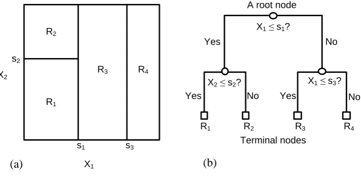
A root node

Figure 1. (a) The partitioning of a two-dimensional feature space into four regions, R1-R4; (b) a decision tree with three splits and four terminal nodes corresponding to the four partitions.

605

606

Figure 2. A layout of the random forest analysis method.

Training dataset L with p input variables

Step 1

Generate sub-datasets, Lb (b=1 – B), by randomly copying observations from the training dataset L

Step 2

Grow a regression tree Tbby recursively repeating the following three sub-steps until the minimum number of observations of each node is reached

- Select m variables randomly from the p variables (m ≤ p)

- Find the best split point among the m variables - Split the node of interest into two nodes

607

608

609

610

611

612

613 614

615

Figure 5 Sensor locations (circle for accelerometers, square for thermistors and triangle for anemometer)

01/08 01/09 01/10

-10 0 10 20 30

Time (month/year)

T

e

m

p

e

ra

tu

re

(

C

)

616

617

618

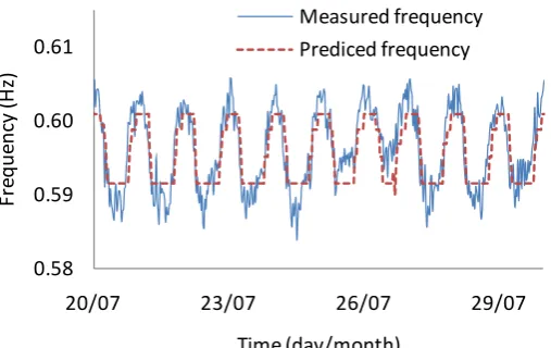
Figure 7. Measured and predicted natural frequencies between July 20 and July 30, 2009 using the multiple linear regression method.

0.58 0.59 0.6 0.61

20/07 23/07 26/07 29/07

Fr

eq

u

en

cy

(H

z)

Time (day/month)

Measured frequency Prediced frequency

Figure 8. Measured and predicted natural frequencies between July 20 and July 30, 2009 using the artificial neural network method.

0.58 0.59 0.6 0.61

20/07 23/07 26/07 29/07

Fr

eq

u

en

cy

(H

z)

Time (day/month)

619

620

621

622

Figure 10. Mean squared errors versus the number of terminal nodes of a tree.

3.8 4.0 4.3 4.5

0 15 30 45 60 75 90

M

ea

n

s

q

u

ar

ed

e

rr

o

r

(x

1

.0

E-6)

Tree size (number of terminal nodes)

Figure 9. Measured and predicted natural frequencies between July 20 and July 30, 2009 using the support vector regression method.

0.58 0.59 0.6 0.61

20/07 23/07 26/07 29/07

Fr

eq

u

en

cy

(H

z)

Time (day/month)

623

624

625

626

Figure 12. Mean squared errors versus number of trees for two cases of 1 and 50 observations in terminal nodes.

3.0 4.0 5.0 6.0 7.0 8.0

0 30 60 90 120

M

ea

n

s

q

u

ar

ed

e

rr

o

r

(x

1

.0

E-6)

Number of trees

1 50

Number of observations in terminal nodes

Figure 11. Measured and predicted natural frequencies between July 20 and July 30, 2009 using the regression tree method.

0.58 0.59 0.60 0.61

20/07 23/07 26/07 29/07

Fr

eq

u

en

cy

(H

z)

Time (day/month)

627

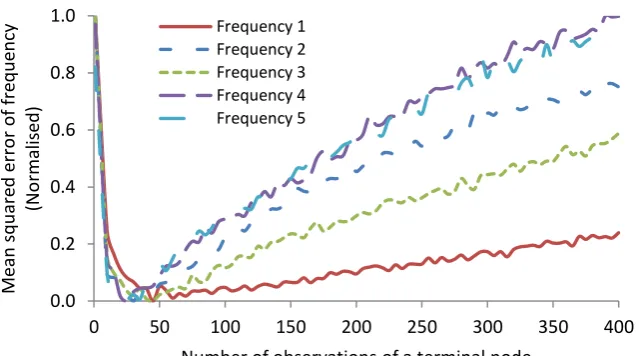
Figure 13. Mean squared errors versus the number of observations in a terminal node

0.0 0.2 0.4 0.6 0.8 1.0

0 50 100 150 200 250 300 350 400

Me

an

squ

ar

ed

error

o

f fre

q

u

en

cy

(No

rm

alis

ed

)

Number of observations of a terminal node

Frequency 1 Frequency 2 Frequency 3 Frequency 4 Frequency 5

Figure 14. Measured and predicted natural frequencies between July 20 and July 30, 2009 using the random forest method

0.58 0.59 0.6 0.61

20/07 23/07 26/07 29/07

Fr

eq

u

en

cy

(H

z)

Time (day/month)

628

629

630

Figure 15. Probability distribution of errors for (a) support vector regression and (b) random forest

-15 -10 -5 0 5 10 15

0 20 40 60 80 100 120 140

Error (x1.0E-3, Hz)

P

ro

b

a

b

il

it

y

d

e

n

si

ty

fu

n

ct

io

n

Observed PDF Theorical PDF

-15 -10 -5 0 5 10 15

0 20 40 60 80 100 120 140

Error (x1.0E-3, Hz)

P

ro

b

a

b

il

it

y

d

e

n

si

ty

fu

n

ct

io

n

Observed PDF Theorical PDF (a)

631

632

633

634

635

Figure 16. Measured and predicted natural frequencies (20 – 30 July, 2009) together with the 95% confidence interval using (a) support vector regression and (b) random forest

0.58 0.59 0.6 0.61 0.62

20/07 23/07 26/07 29/07

Fr

eq

u

en

cy

(H

z)

Time (day/month)

Upper bound of frequency Measured frequency Prediced frequency Lower bound of frequency

0.58 0.59 0.60 0.61 0.62

20/07 23/07 26/07 29/07

Fr

eq

u

en

cy

(H

z)

Time (day/month)

Upper bound of frequency Measured frequency Prediced frequency Lower bound of frequency

(a)

636

637

638

639

Figure 18. Evaluating simultaneous effects of temperature, wind, and traffic loading on the modal frequency responses through the relative importance of variables using the RF method.

0 25 50 75 100

1 2 3 4 5

R

e

lat

ive

im

p

o

rta

n

ce

(

%

)

Frequency number

Temperature Wind Traffic

Figure 17. Evaluating simultaneous effects of temperature, wind, and traffic loading on the natural frequency responses through the relative importance of variables using the MLR method.

0 25 50 75 100

1 2 3 4 5

R

e

lat

ive

im

p

o

rta

n

ce

(

%

)

Frequency number

640

Table 1. Parameters of measured natural frequencies of the bridge.

641

Mode number

Average frequency

(Hz)

Frequency range (Hz) Maximum

difference (%)

Standard deviation

(Hz)

minimum maximum

1 0.39 0.38 0.41 8 0.00

2 0.47 0.41 0.57 34 0.01

3 0.60 0.58 0.61 5 0.01

4 0.69 0.67 0.70 4 0.00

5 0.73 0.71 0.75 6 0.01

642 643 644

Table 2. Results of the MLR method for the first five modes of the bridge

645

Frequency number

Mean squared error (×10-6)

Training set Test set

1 4.0 2.8

2 84.4 99.1

3 20.5 13.7

4 11.7 11.6

5 18.5 23.1

646 647

Table 3. Results of the ANN method for the first five modes of the bridge

648

Frequency number Number of hidden

nodes

Mean squared error (×10-6)

Training set Test set

1 11 3.9 2.7

2 10 87.6 95.7

3 21 22.8 12.3

4 33 15.7 18.6

5 21 19.5 20.0

649 650

Table 4. Results of the SVR method for the first five modes of the bridge

651

Frequency number   Mean squared error (×10

-6₎

Training set Test set

1 20 0.8 3.7 2.5

2 9 0.17 69.5 96.7

3 20 0.56 16.6 11.8

4 12 0.28 9.4 10.6

5 14 0.36 15.7 18.6