warwick.ac.uk/lib-publications
Original citation:
Adams, Stefan, Kister, Alexander Karl and Weber, Hendrik. (2016) Sample path large
deviations for Laplacian models in (1+1)-dimensions. Electronic Journal of Probability, 21 .
62.
Permanent WRAP URL:
http://wrap.warwick.ac.uk/82947
Copyright and reuse:
The Warwick Research Archive Portal (WRAP) makes this work of researchers of the
University of Warwick available open access under the following conditions.
This article is made available under the Creative Commons Attribution 4.0 International
license (CC BY 4.0) and may be reused according to the conditions of the license. For more
details see: http://creativecommons.org/licenses/by/4.0/
A note on versions:
The version presented in WRAP is the published version, or, version of record, and may be
cited as it appears here.
El e c t ro n ic
J
o f
P
r o
b a bi l i t y
Electron. J. Probab.21(2016), no. 62, 1–36. ISSN:1083-6489 DOI:10.1214/16-EJP8
Sample path large deviations for Laplacian models in
(1 + 1)
-dimensions
Stefan Adams
*Alexander Kister
†Hendrik Weber
‡Abstract
We study scaling limits of a Laplacian pinning model in (1 + 1) dimension and derive sample path large deviations for the profile height function. The model is given by a Gaussian integrated random walk (or a Gaussian integrated random walk bridge) perturbed by an attractive force towards the zero-level. We study in detail the behaviour of the rate function and show that it can admit up to five minimisers depending on the choices of pinning strength and boundary conditions. This study complements corresponding large deviation results for Gaussian gradient systems with pinning in(1 + 1)-dimension ([FS04]) in(1 +d)-dimension ([BFO09]), and recently in higher dimensions in [BCF14].
Keywords:Large deviation; Laplacian models; pinning; integrated random walk; scaling limits; bi-harmonic.
AMS MSC 2010:Primary 60K35, Secondary 60F10; 82B41.
Submitted to EJP on February 5, 2016, final version accepted on October 3, 2016.
1
Introduction and large deviation results
1.1 The models
We are going to study models for(1 + 1)-dimensional random fields. These models are defined in terms of the potential, a measurable functionV: R→R∪ {+∞}such that x7→exp(−V(x))is bounded and continuous and that
Z
R
e−V(x)dx <∞ and
Z
R
x2e−V(x)dx=:σ2<∞ and
Z
R
xe−V(x)dx= 0.
For most of the article we consider the Gaussian caseV(x) = 12x2. Given the potential
V, we define a Hamiltonian H[`,r](φ), defined for `, r ∈ Z, with r−` ≥ 2, and for
φ: {`, `+ 1, . . . , r−1, r} →Rby
H[`,r](φ) :=
r−1 X
k=`+1
V(∆φk), (1.1)
*Mathematics Institute, University of Warwick, Coventry CV4 7AL, United Kingdom. E-mail:s.adams@
warwick.ac.uk
where∆denotes the discrete Laplacian,∆φk=φk+1+φk−1−2φk. Our pinning models are then given by the probability measures
γN,εψ (dφ) = 1 ZN,ε(ψ)
e−H[−1,N+1](φ)
N−1 Y
k=1
(εδ0(dφk) + dφk)
Y
k∈{−1,0,N,N+1}
δψk(dφk),
γψf
N,ε(dφ) = 1 ZN,ε(ψf)
e−H[−1,N+1](φ)
N+1 Y
k=1
(εδ0(dφk) + dφk)
Y
k∈{−1,0}
δψk(dφk),
(1.2)
whereN ≥2is an integer,ε≥0is the pinning strength,dφkis the Lebesgue measure on
R,δ0is the Dirac mass at zero, whereψ∈RZis a given boundary condition andZN,ε(ψ) (resp. ZN,ε(ψf)) is the normalisation, which is usually called partition function.
The measures given in (1.2) are (1 + 1)-dimensional models for a linear chain of lengthN which is attracted to the defect line, thex-axis. The parameterε≥0 tunes the strength of the attraction and one wishes to understand its effect on the field, in the largeN limit. The models withε = 0have no pinning reward at all and are thus free Laplacian models. By “(1 + 1)-dimensional” we mean that the configurations of the chain are given by graphs{(k, φk)}−1≤k≤N+1. Models with Laplacian interaction
have been studied in the Physics literature in the context of semiflexible polymers, c.f. [BLL00, HV09], or in the context of deforming rods in space, cf. [Ant05].
The basic properties of the models were investigated in the two papers [CD08, CD09], to which we refer for a detailed discussion and for a survey of the literature. In particular, it was shown in [CD08] that there is a critical valueεc ∈(0,∞)that determines a phase
transitions between adelocalised regime (ε < εc), in which the reward is essentially
ineffective, and alocalised regime (ε > εc), in which the reward has a macroscopic
effect on the field. For more details see Section 1.2.3 below. In the present paper we derive large deviation principles for the macroscopic empirical profile distributed under the measures in (1.2) (Section 1.2). The corresponding large deviation results for the gradient models, where the Hamiltonian is a function of the discrete gradient of the field instead of the discrete Laplacian, have been derived in [FS04] for Gaussian random walk bridges inRand for Gaussian random walks and bridges in higher dimensions in [BFO09]. In [FO10] large deviations for general non-Gaussian random walks inRd, d≥1, were analysed, and in [BCF14] gradient models in higher (lattice) dimensions were introduced.
A common feature of all these gradient models is, that typical fluctuations are observed on scale√N and that large deviation results can be obtained on a linear scale inN; for more details see [Fun05]. In contrast in the Laplacian case the scale for the scaling limits isN3/2as already observed in Sinai’s work [Sin92] on integrated random
walks and proved in the specific context of our models by Caravenna and Deuschel in [CD09]. In this article we derive large deviations principles on scaleN2. Beyond the different scaling, a major technical difference between the Laplacian case and the gradient case is the fact that the Markov property which features prominently in the large deviation proofs in the gradient case [FS04, BFO09] is not directly available in the Laplacian case. To overcome this difficulty we introduce a correction technique and replace “single zeros” of the profile by “double zeros” which then allows us to write the distribution over disjoint intervals separated by a double zero as the product of independent distributions over the disjoint intervals.
minimising the macroscopic bi-Laplacian energy (see Appendix A). Once the pinning reward is switched on, the integrated random walk (scaled random field) has essentially two different strategies to pick up reward. One strategy is to start picking up the reward earlier despite the energy involved to bend to the zero line with speed zero and the other strategy is to cross the zero level producing a longer bend before turning to the zero level and picking up reward. The choice of pinning strength and boundary conditions determines which of these strategies is favoured by the rate function.
In Section 1.2 we present the large deviation results which are proved in Section 3. The results of the variational analysis are given in Section 2 and their proofs are given in Section 2.3. We include an Appendix A where some basic facts about the bi-harmonic equation and bi-harmonic functions along with convergence statements for the discrete bi-Laplacian are provided. In Appendix B we collect some well-known facts about partition functions of Gaussian integrated random walks.
1.2 Sample path large deviations 1.2.1 Empirical profile
LethN ={hN(t) :t∈[0,1]}be the macroscopic empirical profile determined from the microscopic height functionφunder the proper scaling. More precisely, definehN as a linear interpolation of(hN(k/N) =φk/N2)k∈ΛN withΛN ={−1,0, . . . , N, N+ 1}by
hN(t) =
bN tc −N t+ 1
N2 φbN tc+
N t− bN tc
N2 φbN tc+1, t∈[0,1]. (1.3)
We study hN distributed under the measures given in (1.2) endowed with a suitable boundary conditionsψ(N). In the case of Dirichlet boundary conditions, we fix parameters
a, α, b, β∈Rand then define the microscopic boundary conditions as
ψ(N)(x) =
aN2−αN ifx=−1,
aN2 ifx= 0,
bN2 ifx=N,
bN2+βN ifx=N+ 1,
0 otherwise.
(1.4)
On the macroscopic scale this choice corresponds to fixinghN(0) =aandhN(1) =bas well the discrete derivatives
˙
hN(0) =
ψ(N)(0)−ψ(N)(−1)
N =α and
˙
hN(1) =
ψ(N)(N+ 1)−ψ(N)(N)
N =β.
In the case of free boundary conditions on the right hand side we only specify the boundary inx=−1andx= 0, and writeψ(N)
f (−1) =aN
2−αN andψ(N)
f (0) =aN
2, see
(1.2). We writer= (a, α, b, β)to specify our choice of boundary conditionsψ(N) in the
Dirichlet case anda= (a, α)for the mixed Dirichlet and free boundary case. We denote the Gibbs distributions withε= 0(no pinning) byγr
N for Dirichlet boundary conditions and byγa
N for Dirichlet boundary conditions on the left and free boundary conditions on the right and their partition functions byZN(r)andZN(a), respectively. In Section 1.2.2 we study the large deviation principles without pinning (ε= 0) for general integrated random walks with free boundary conditions on the right hand side and show that these results apply to Gaussian integrated random walk bridges as well. Our main large deviation result for the measures with pinning are then presented in Section 1.2.3. To state these results we introduce the spaces
Hr2={h∈H2([0,1]) :h(0) =a, h(1) =b,h˙(0) =α,h˙(1) =β},
Ha2={h∈H2([0,1]) :h(0) =a,h˙(0) =α}
used in the case of free boundary conditions on the right. Here,H2([0,1])is the usual Sobolev space. We write C([0,1];R) for the space of continuous functions on [0,1] equipped with the supremum norm.
1.2.2 Large deviations for integrated random walks and Gaussian integrated random walk bridges
We recall the integrated random walk representation in Proposition 2.2 of [CD08]. Let (Xk)k∈Nbe a sequence of independent and identically distributed random variables, with marginal lawsX1∼exp(−V(x))dx, and(Yn)n∈N0 the corresponding random walk with
initial conditionY0=αNandYn =αN+X1+· · ·+Xn. The integrated random walk is
denoted by(Zn)n∈N0 withZ0=aN
2andZ
n =aN2+Y1+· · ·+Yn. We denotePa the probability distribution of the above defined processes. Then the following holds for the above defined class of potentialsV.
Proposition 1.1([CD08]).The pinning free modelγNr (ε= 0) is the law of the vector (Z1, . . . , ZN−1) under the measure Pr(·) := Pa(·|ZN = bN2, ZN+1 = bN2+βN). The
partition functionZN(r) is the value at(βN, bN2+βN)of the density of the vector (YN+1, ZN+1)under the law Pa. The model γNa coincides with the integrated random
walkPa.
The first part of the following result is the generalisation of Mogulskii’s theorem [Mog76] from random walks to integrated random walks whereas its second part is the generalisation to Gaussian integrated random walk bridges.
Theorem 1.2. (a) LetV be any potential of the form above such that
Λ(λ) := logE[ehλ,X1i]<∞ (1.5)
for allλ∈R, then the following holds. The large deviation principle (LDP) holds forhN underγNa on the spaceC([0,1];R)asN → ∞with speedN and the unnor-malised good rate functionEf of the form:
Ef(h) =
(R1 0 Λ
∗(¨h(t)) dt, ifh∈H2
a,
+∞ otherwise. (1.6)
HereΛ∗denotes the Fenchel-Legendre transform ofΛ.
(b) ForV(η) = 12η2the following holds. The large deviation principle (LDP) holds forh
N underγr
N on the spacesC([0,1];R)asN → ∞with speedN and the unormalised good rate functionE of the form:
E(h) =
(1 2
R1 0 ¨h
2(t) dt, ifh∈H2
r,
+∞ otherwise. (1.7)
Remark 1.3. (a) The rate functions in both cases are obtained from the unnormalised rate functions byI0
f(h) =Ef(h)−infg∈H2
aEf(g)for general integrated random walks
with potentialV respectively byI0(h) =E(h)−inf
g∈H2
rE(g)for Gaussian integrated
random walk bridges.
(b) We believe that the large deviation in Theorem 1.2(b) holds for general potentials
1.2.3 Large deviations for pinning models
The large deviation principle for the pinning models gets an additional term for the rate function. Recall that the logarithm of the partition function is the free energy. Difference of the free energies with pinning and without pinning for zero boundary conditions(r=0) will be an important ingredient in our rate functions. We defineτ(ε) as the thermodynamic limit of the logarithm of the quotient of the partition function with pinning and the partition function without pinning (both with zero boundary condition),
τ(ε) = lim
N→∞
1 N log
ZN,ε(0)
ZN(0)
. (1.8)
The existence of the limit in (1.8) and its properties have been derived by Caravenna and Deuschel in [CD08], we summarise their result in the following proposition.
Proposition 1.4([CD08]).The limit in (1.8)exist for everyε≥0. Furthermore, there existsεc∈(0,∞)such thatτ(ε) = 0forε∈[0, εc], while0< τ(ε)<∞forε∈(εc,∞), and
asε→ ∞,
τ(ε) = logε(1−o(1)).
Moreover the functionτ is real analytic on(εc,∞).
We have the following sample path large deviation principles forhN underγrN,εand
γa
N,ε, respectively. The unnormalised rate functions denoted byΣ
εandΣε
fare of the form
Σε(h) = 1 2
Z 1
0
¨
h2(t) dt−τ(ε)|{t∈[0,1] :h(t) = 0}|, (1.9)
forh∈H =Hr2andH =Ha2, respectively. Here| · |stands for the Lebesgue measure.
Theorem 1.5.LetV(η) = 12η2. The LDP holds forh
N underγN =γN,εr , γN,εa respectively on the spaceC([0,1];R)asN → ∞with the speedN and the good rate functionsI=Iε andI=Ifεof the form:
I(h) =
(
Σ(h)−infh∈H{Σ(h)}, ifh∈H,
+∞ otherwise, (1.10)
with Σ = Σε and Σ = Σε
f respectively, and H = Hr2 respectively H = Ha2. Namely, for every open setO and every closed setK ofC([0,1];R)equipped with the uniform topology, we have that
lim inf N→∞
1
N logγN(hN ∈O)≥ −hinf∈OI(h),
lim sup N→∞
1
N logγN(hN ∈K)≤ −hinf∈K I(h), (1.11)
in each of two situations.
As the limitτ(ε)of the difference of the free energies appears in our rate functions it is worth pointing out that this has a direct translation in terms of path properties of the field, see [CD08]. This is the microscopic counterpart of the effect of the reward term in our pinning rate functions. Defining the contact number`N by
`N := #{k∈ {1, . . . , N}:φk= 0},
we can easily obtain that forε >0(see [CD08]),
DN(ε) :=Eγ0
N,ε
This gives the following paths properties. When ε > εc, thenDN(ε) → D(ε) > 0 as
N → ∞, and the mean contact density is non-vanishing leading to localisation of the field (integrated random walk respectively integrated random walk bridge). For the other case,ε < εc, we getDN(ε)→0asN → ∞and thus the contact density is vanishing in the thermodynamic limits leading to de-localisation.
2
Minimisers of the rate functions
We are concerned with the setMεof the minimiser of the unnormalised rate functions in (1.9) for our pinning LDPs. Any minimiser of (1.9) is a zero of the corresponding rate function in Theorem 1.5. We leth∗r ∈ Hr2 be the unique minimiser of the energy
E defined in (1.7) (see Proposition A.1), that is, E(h) = 1/2R01¨h2(t) dt is the energy of the bi-Laplacian in dimension one. For any intervalI ⊂ [0,1]we let h∗,I
r ∈ Hr2(I), where the boundary conditions apply to the boundaries ofI, be the unique minimiser ofEI(h) =1
2 R
I h¨
2(t) dt, and we sometimes writea,bfor the boundary conditionrwith
a= (a, α)andb= (b, β). Of major interest are the zero sets
Nh={t∈[0,1] :h(t) = 0} of any minimiserh.
In Section 2.1 we study the minimiser for the case of Dirichlet boundary conditions on the left hand side and free boundary conditions on the right hand side, in Section 2.2 we summarise our findings for the Dirichlet boundary case on both the right hand and left hand side. In Section 2.3 we give the proofs for our statements.
2.1 Free boundary conditions on the right hand side
We consider Dirichlet boundary conditions on the left hand side and the free boundary condition on the right side only.
LetMε
f denote the set of minimiser ofΣεf.
Proposition 2.1.For any boundary conditiona= (a, α)on the left hand side the set
Mε
f of minimiser ofΣ ε
f is a subset of
{h} ∪ {h`:`∈(0,1)}, (2.1)
where for any`∈(0,1)the functionsh`∈Ha,f2 are given by
h`(t) =
(
h∗(a,,(00,`))(t) , fort∈[0, `),
0 , fort∈[`,1]; (2.2)
and the functionh∈H2
ais the linear functionh(t) =a+αt, t∈[0,1].
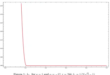
Note thathdoes not pick up reward for any boundary conditiona6=0whereas for
a =0it takes the maximal reward. The functionh` picks up the reward in[`,1], see Figure 1,2,3. This motivates the following definitions. For anyτ∈Randa∈R2we let
Eτ
(a,0)(`) =E(h ∗,(0,`)
a,0 ) +τ `, (2.3)
and observe that forτ=τ(ε)
Σεf(h`) =E τ(ε)
(a,0)(`)−τ(ε). (2.4)
Henceforth minimiser ofΣε
f are given by functions of typeh`only if`is a minimiser of the functionEτ
(a,0)in[0,1]. We collect an analysis of the latter function in the next
0.0 0.2 0.4 0.6 0.8 1.0 0.000
[image:8.595.112.489.92.349.2]0.005 0.010 0.015 0.020 0.025 0.030 0.035
Figure 1:h`1 fora= 1andα=−12, τ = 288, `1= 1/2( √
2−1)
Proposition 2.2(Minimiser forE(τa,0)). (a) Forτ = 0 the functionE0
(a,0) is strictly
decreasing withlim`→∞E(0a,0)(`) = 0.
(b) Forτ >0 the functionE(τa,0,0), a 6= 0, has one local minimum at ` =`1(τ, a,0) = p
|a|(18/τ)1/4, and the function E(0τ,α,0), α 6= 0, has one local minimum at ` =
`1(τ,0, α) = q
2
τ|α|. In both cases there existτ1(a)such that`1(τ,a) ≤1 for all
τ ≥τ1(a).
(c) For τ > 0 and a = (a, α) ∈ R2 with w = |a|/|α| ∈ (0,∞) ands = sign (aα) the
functionE(τa,0)has one local minimum at`=`1(τ,a) =√12τ |α|+ q
α2+ 6|a|√2τ
whens= 1, whereas fors =−1 the functionE(τa,0)has two local minima at`=
`1(τ,a) = √12τ − |α|+ q
α2+ 6|a|√2τ
and`=`2(τ,a) =√12τ |α|+ q
α2−6|a|√2τ
,
where`2is a local minimum only ifτ≤ α
4
72a2. In all cases there areτi(a)such that
`i(τ,a)≤1for allτ≥τi(a),i= 1,2.
From now we use the notation for `1 and `2 for the points where the functions
h`i, i= 1,2, pick up reward. We shall study the zero sets of all minimiser, that is we need to check ifh`has zeroes in[0, `)before picking up the reward in[`,1].
Lemma 2.3.Leta >0, then the functionsh(∗a,α,,(0,`0))with α >0, h∗(0,(0,α,,`0))withα6= 0, and
h∗(a,,(0−,`α,)0)withα`/a∈[0,3)have no zeroes in(0, `), whereas the functionsh∗(a,,(0−,`α,)0)with
α`/a >3have exactly one zero in(0, `). Analogous statements hold fora <0.
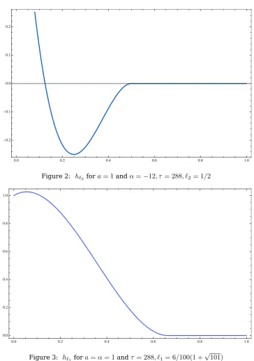
There is a qualitative difference between the minimiserh`1andh`2as the latter one
has a zero before picking up the reward on[`2,1], see Figure 2.
In the following we writeεi(a)for the value of the reward withτ(εi(a)) =τi(a)such that`i(τi(a),a)≤1, i= 1,2.
Theorem 2.4(Minimiser forΣε
f). (a) If a = (a,0), a = 06 or a = (0, α), α 6= 0 or
0.0 0.2 0.4 0.6 0.8 1.0
-0.2
-0.1 0.0 0.1 0.2
Figure 2: h`2 fora= 1andα=−12, τ = 288, `2= 1/2
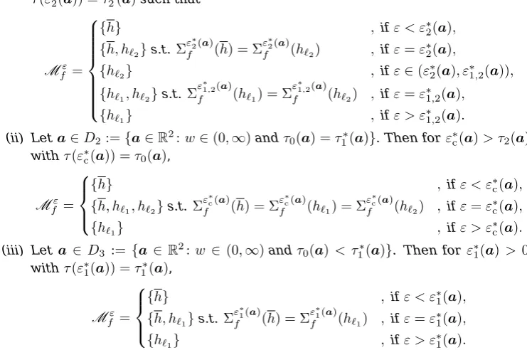
0.0 0.2 0.4 0.6 0.8 1.0
[image:9.595.115.480.86.605.2]0.0 0.2 0.4 0.6 0.8 1.0
Figure 3: h`1 fora=α= 1andτ= 288, `1= 6/100(1 + √
101)
Mε f =
{h} , ifε < ε∗(a),
{h, h`1}s.t.Σ
ε∗
f (h) = Σ
ε∗
f (h`1) , ifε=ε ∗(a),
{h`1} , ifε > ε
∗(a).
(b) Assumew = |a|/|α| ∈ (0,∞) ands = sign (aα) = −1. There are τ0(a) > 0 and
τ∗
1(a)>0andτ2∗(a)>0such that the following statements hold.
(i) Let a ∈ D1 := {a ∈ R2:w ∈ (0,∞)andτ0(a) > τ1∗(a)}. Then there exist
τ(ε∗2(a)) =τ2∗(a)such that Mε f =
{h} , ifε < ε∗2(a),
{h, h`2}s.t.Σ
ε∗
2(a)
f (h) = Σ
ε∗
2(a)
f (h`2) , ifε=ε ∗ 2(a),
{h`2} , ifε∈(ε
∗
2(a), ε∗1,2(a)), {h`1, h`2}s.t.Σ
ε∗1,2(a)
f (h`1) = Σ
ε∗1,2(a)
f (h`2) , ifε=ε ∗ 1,2(a),
{h`1} , ifε > ε
∗ 1,2(a).
(ii) Leta∈D2:={a∈R2:w∈(0,∞)andτ0(a) =τ1∗(a)}. Then forε∗c(a)> τ2(a)
withτ(ε∗c(a)) =τ0(a),
Mε f =
{h} , ifε < ε∗c(a),
{h, h`1, h`2}s.t.Σ
ε∗c(a)
f (h) = Σ
ε∗c(a)
f (h`1) = Σ
ε∗c(a)
f (h`2) , ifε=ε ∗ c(a),
{h`1} , ifε > ε
∗ c(a).
(iii) Leta ∈ D3 := {a ∈R2: w ∈ (0,∞)andτ0(a)< τ1∗(a)}. Then for ε∗1(a) >0
withτ(ε∗1(a)) =τ1∗(a),
Mε f =
{h} , ifε < ε∗
1(a), {h, h`1}s.t.Σ
ε∗1(a)
f (h) = Σ
ε∗1(a)
f (h`1) , ifε=ε ∗ 1(a),
{h`1} , ifε > ε
∗ 1(a).
[image:10.595.124.495.107.353.2]Remark 2.5.We have seen that the rate function Σεf can have up to three distinct global minimisers. See Figure 1-2 for examples of these functions. The minimiser in Figure 1 has no isolated zero before picking up the reward. Note that the existence of the minimiser (see Figure 2) with a single zero before picking up a reward depends on the choice boundary conditions. This minimiser only exist if the gradient at0has opposite sign of the value at zero. See Figure 3 for an example when the gradient has the same sign as the value of the function at zero. The minimiserh`1 is the global minimiser
if the reward is sufficiently large.
2.2 Dirichlet boundary
We consider Dirichlet boundary conditions on both sides given by the vectorr = (a, α, b, β) = (a,b). In a similar way to Section 2.1 for free boundary conditions on the right hand side we define functionsh`,r∈Hr2for any`, r≥0with`≤rand`+r≤1by
h`,r(t) =
h∗a,,(00,`)(t) , t∈[0, `),
0 , t∈[`,1−r],
h∗0,,b(1−r,1)(t) , t∈(1−r,1].
(2.5)
Furthermore, we define the following energy function depending only on`andr,
E(`, r) =E(ha,∗,(00,`)) +E(h0∗,,b(1−r,1))−τ(ε)(1−`−r), (2.6)
and using (2.3) we get
E(`, r) =E(τa,(ε0))(`) +E(τ0(,b,βε) )(r)−τ(ε) =E(τa,(ε0))(`) +E(τb,(ε−)β,0)(r)−τ(ε), (2.7)
whereβ is replaced by−βdue to symmetry, that is, using that
h∗(0,(1,b−)r,1)(t) =h∗(b,,(1−−β,r,01))(2−r−t) =h(∗b,,(0−,rβ,)0)(1−t)
fort∈[1−r,1]. Hence
Σε(h`,r) =E(`, r).
For given boundaryr= (a, α, b, β)the functionh∗r ∈H2
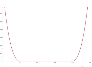
0.2 0.4 0.6 0.8 1.0 0.1
[image:11.595.120.476.76.337.2]0.2 0.3 0.4 0.5 0.6
Figure 4:h`1fora=b= 1andα=−12, β= 12, τ = 288, `1= 1/2( √
2−1)
Proposition 2.6.For any Dirichlet boundary conditionr∈R4the setMεof minimiser of the rate functionΣεinH2
r is a subset of
{h`,r, h∗r:`+r≤1},
where`andrare minimiser ofEτ(ε)in Proposition 2.2.
Proposition 2.6 allows to reduce the optimisation of the rate function Σε to the minimisation of the functionEdefined in (2.7) for0≤`+r≤1. The general problem involves up to five parameters including the boundary conditionsr∈R4and the pinning free energyτ(ε)for the rewardε. It involves studying several different sub cases and in order to demonstrate the key features of the whole minimisation problem we study only a special case in the following and only outline how any general case can be approached.
Thesymmetric case r= (a, α, a,−α): It is straightforward to see that
Σε(h`i,`j) =E(`i, `j) =E τ(ε)
(a,α,0)(`i) +E τ(ε)
(a,α,0)(`j)−τ(ε), i, j= 1,2. (2.8) See figure 4 and figure 5 for examples of the minimiser h`1,`1 andh`2,`2 respectively.
Clearly the unique minimiserh∗r(t) =a+αt−αt2ofE has the symmetry
h∗r(1/2−t) =h∗r(1/2 +t)
fort∈[0,1/2]. The functionEis not convex and thus we distinguish two different sets of parameter(a, τ(ε))∈R3according to whether (i)`i(τ(ε),a)≤1/2fori= 1,2; or whether (ii)`2(τ(ε),a)>1/2> `1(τ(ε),a). There are no other cases for the parameter due to the
condition`1+`2≤1and the fact that`2(τ(ε),a)> `1(τ(ε),a).
Parameter regime (i):
D1:={(a, τ)∈R3:`1(τ,a)≤1/2 ∧`2(τ,a)≤1/2if`2(τ,a)is local minimum ofE(τa,0)}.
Parameter regime (ii):
D2:={(a, τ)∈R3: 1≥`2(τ(ε),a)>1/2> `1(τ(ε),a)>0, τ ≤
α4 72a2}.
0.0 0.2 0.4 0.6 0.8 1.0
[image:12.595.120.480.84.326.2]-0.2 0.0 0.2 0.4 0.6 0.8 1.0
Figure 5: h`2 fora=b= 1andα=−12, β= 12, τ = 288, `2= 1/2
There areεi(a)such that`i(τ(ε),a) ≤1/2for all ε≥εi(a), i = 1,2. We denote by
τ1∗(a) =τ(ε∗1(a))the unique value ofτsuch that
Eτ∗
1(a)(`1(τ∗
1(a),a))−1/2τ1∗(a) = 1/2E(h∗r). (2.9)
Likewise, we denoteτ2∗(a)the unique value ofτ such that
Eτ∗
2(a)(`
1(τ2∗(a),a))−1/2τ2∗(a) = 1/2E(h∗r)
when such a value exists inRotherwise we putτ2∗(a) =∞. We denoteτ0(a)the unique
zero in Lemma 2.10 (a) of the difference∆(τ) =Eτ(`1(τ,a))−Eτ(`2(τ,a)).
Theorem 2.7(Minimiser forΣε, symmetric case).Letr= (a, α, a,−α).
(a) If a= (a,0), a6= 0,ora = (0, α), α 6= 0,orw=|a|/|α| ∈(0,∞)withsign (aα) = 1 andε≥ε1(a), then(a, τ(ε))∈D1and there isε∗1(a)> ε1(a)such that
Mε=
{h∗r} , ifε < ε∗1(a),
{h∗
r, h`1,`1}s.t.Σ
ε∗1(a)(h∗
r) = Σε
∗
1(a)(h`
1,`1) , ifε=ε ∗ 1(a),
{h`1,`1} , ifε > ε
∗ 1(a).
(b) Assumew = |a|/|α| ∈ (0,∞) ands = sign (aα) = −1. There are τ0(a) > 0 and
τ1∗(a)>0andτ2∗(a)>0such that the following statements hold.
[(i)]Let a ∈ D1 := {a ∈ R2: w ∈ (0,∞)andτ0(a) > τ1∗(a)}. Then there exists
e
ε1,2(a) > 0 such that(a, τ(ε)) ∈ D2 for all ε ∈ (εe1,2(a), ε2(a))and (a, τ(ε)) ∈ D1
forε≥ε2(a). Then there existε∗1,2(a)>0andε2∗(a)>0with ε∗2(a)< ε∗1,2(a)and
Mε=
{h∗r} , ifε <eε1,2(a),
{h∗r, h`2,`1}s.t.Σ
ε(h∗
r)≤Σε(h`2,`1)or
Σε(h∗
r)>Σε(h`2,`1) , ifε∈(εe1,2(a), ε2(a)), {h∗r, h`2,`2}s.t.Σ
ε∗2(a)(h∗
r) = Σε
∗
2(a)(h`
2,`2) , ifε=ε ∗ 2(a),
{h`2,`2} , ifε∈(ε
∗
2(a), ε∗1,2(a)), {h`1,`1, h`2,`2}s.t.Σ
ε∗1,2(a)(h
`1,`1) = Σ
ε∗1,2(a)(h
`2,`2) , ifε=ε ∗ 1,2(a),
{h`1,`1} , ifε > ε
∗ 1,2(a).
[(ii)]Leta ∈D2 := {a ∈ R2:w ∈ (0,∞)andτ0(a) = τ1∗(a)}. Then there exists
e
ε1,2(a)>0such that(a, τ(ε))∈D2for allε∈(εe1,2(a), ε2(a))and(a, τ(ε))∈D1for
ε≥ε2(a). Then there existsε∗c(a)>0withτ(ε∗c(a)) =τ0(a)andεc∗(a)≥ε2(a)such
that
Mε=
{h∗r} , ifε <εe1,2(a),
{h∗r, h`2,`1}s.t.Σ
ε(h∗
r)≤Σ ε(h
`2,`1)or
Σε(h∗
r)>Σε(h`2,`1) , ifε∈(εe1,2(a), ε2(a)), {h∗r} , ifε∈(ε2(a), ε∗c(a)), {h∗r, h`1,`1, h`2,`2, h`1,`2, h`2,`1}s.t.
Σε∗c(a)(h∗
r) = Σε
∗
c(a)(h`
1,`1) = Σ
ε∗c(a)(h
`2,`2)
= Σε∗c(a)(h`
1,`2) = Σ
ε∗
c(a)(h`
2,`1) , ifε=ε ∗ c(a),
{h`1,`1} , ifε > ε
∗ c(a).
[(iii)]Leta ∈D3 :={a ∈R2: w∈ (0,∞)andτ0(a)< τ1∗(a)}. Then there exists
e
ε1,2(a)>0such that(a, τ(ε))∈D2for allε∈(εe1,2(a), ε1(a))and(a, τ(ε))∈D1for
ε≥ε1(a). Then there existsε∗1(a)> ε1(a)withτ(ε∗1(a)) =τ1∗(a)such that
Mε=
{h∗r} , ifε <εe1,2(a),
{h∗r, h`2,`1}s.t.Σ
ε(h∗
r)≤Σε(h`2,`1)or
Σε(h∗
r)>Σε(h`2,`1) , ifε∈(εe1,2(a), ε ∗ 1(a)), {h∗r, h`1,`1}s.t.Σ
ε∗1(a)(h∗
r) = Σε
∗
1(a)(h`
1) , ifε=ε ∗ 1(a),
{h`1,`1} , ifε > ε
∗ 1(a).
Remark 2.8(General boundary conditions).For general boundary conditionsr= (a, α, b, β)one can apply the same techniques as for the symmetric case. Thus minimiser
ofΣεare elements of
{h∗r, h`,`, hr,r, h`,r, hr,`:`+r≤1}.
Remark 2.9 (Concentration of measures).The large deviation principle in Theo-rem 1.5 immediately implies the concentration properties forγN =γN,εr andγN =γN,εa :
lim
N→∞γN(dist∞(hN,M
ε)≤δ) = 1, (2.10)
for everyδ >0, whereMε={h∗:h∗minimiser ofI}withI=IεandI=Iε
f, respectively, anddist∞denotes the distance underk·k∞. More precisely, for anyδ >0there exists
c(δ)>0such that
γN(dist∞(hN,Mε)> δ)≤e−c(δ)N
for large enoughN. We say that two functionh1, h2∈Mεcoexist in the limitN → ∞
underγN with probabilitiesλ1, λ2>0, λ1+λ2= 1when
lim
hold for small enoughδ >0. The same applies to the free boundary case on the right hand side and its set of minimiserMε
f. For gradient models with quadratic interaction (Gaussian) the authors in [BFO09] have investigated this concentration of measure problem and obtained statements depending on the dimension m of the underlying random walk (i.e.(1 +m)-dimensional models). The authors are using finer estimates than one employs for the large deviation principle, in particular the make use of a renewal property of the partition functions. In our setting of Laplacian interaction the renewal structure of the partition functions is different and requires different type of estimates. In addition, the concentration of measure problem requires to study all cases of possible minimiser. This is studied in ([A16]).
2.3 Proofs: variational analysis 2.3.1 Free boundary condition
Proof of Proposition 2.1. Suppose thath∈H2
ais not element of the set (2.1). It is easy to see that there is at least one functionh∗ in the set (2.1) with
Σεf(h∗)<Σεf(h). (2.11)
ForΣε
f(h)<∞, we distinguish two cases. If|Nh|= 0, then|Nh|= 0and we get
Σεf(h) =E(h)>0 =E(h) = Σεf(h)
by noting thathis the unique function withE(h) = 0. If|Nh|>0we argue as follows. Let`be the infimum andrbe the supremum of the accumulation points ofNh, and note that`, r∈Nh. Since|Nh∩[`, r]c|= 0we have
Σεf(h) =E[0,`](h) +E(`,r)(h)−τ(ε)|{t∈(`, r) :h(t) = 0}|+E[r,1](h).
As`, r∈Nhwe have thath˙(`) = ˙h(r) = 0as the differential quotient vanishes due to the fact that`andrare accumulations points ofNh. Thus the restrictions ofhandh∗=h` to[0, `]are elements ofH2
(a,0). By the optimality ofh ∗,(0,`)
(a,0) inequality (2.11) is satisfied
forh∗=h`.
Proof of Proposition 2.2. The following scaling relations hold for` >0(in our cases
`∈(0,1)) anda= (a, α),
h∗(a,,(00,`))(t) =h(∗a,`α,,(0,1)0)(t/`) fort∈[0, `]. (2.12)
Using this and Proposition A.1 withr= (a, `α,0,0)we obtain
E(0,`)(h∗,(0,`) (a,0) ) =
1 2`3
Z 1
0
¨ h∗
r(t)
2
dt= 1
`3 6a
2+ 6aα`+ 2α2`2
,
and thus
Eτ
(a,0)(`) =
1 `3 6a
2+ 6aα`+ 2α2`2+τ `,
d d`E
τ
(a,0)(`) =−
18a2
`4 −
12aα
`3 −
2α2
`2 +τ=−
2
`4(3a+α`− p
τ /2`2)(3a+α`+pτ /2`2),
d2 d`2E
τ
(a,0)(`) =
4
`5(6a+α`)(3a+α`).
The derivative has the following zeroes
`1/2=
α±pα2+ 6a√2τ √
2τ ,
`3/4=
−α±pα2−6a√2τ √
2τ .
(a) Our calculations (2.13) imply d
d`E(a,0)(`)<0fora∈R
2\{0}andlim
`→∞E(a,0)(`) =
0. Ifa=α= 0, thenE(0,0,0)(`) = 0for all`.
(b) If a 6= 0 and α = 0 our calculations (2.13) imply that the function has local
minimum at`=`1(τ,a) = p
|a| 18
τ
1/4
, whereas fora= 0andα6= 0the function has local minimum at`=`1(τ,a) =
p
2/τ|α|.
(c) Let w =|a|/|α| ∈ (0,∞)ands = 1. Then (2.13) shows that the function has a
local minimum at ` = `1(τ,a) = √12τ(|α|+ q
α2+ 6|a|√2τ). If s = −1 we get a local
minimum at` = `1(τ,a) = √12τ(−|α|+ q
α2+ 6|a|√2τ)and in case τ ≤ α4
72a2 a second
local minimum at`=`2(τ,a) = √12τ(|α|+ q
α2−6|a|√2τ). Note that`
1(τ,a)< `2(τ,a)
whenever`2(τ,a)is local minimum. This follows immediately from the second derivative
which is positive whenever`i(τ,a)≤|3αa|or`i(τ,a)≥ |6αa| fora >0> αandi= 1,2.
Proof of Lemma 2.3. We are using the scaling property
h∗(a,,(00,`))(t) =ah∗(1,(0,sw,1)−1`,0)(t/`) fora6= 0andt∈[0, `], s= sign (aα), w=|a|/|α|,
h∗(a,,(00,`))(t) =h∗(0,(0,α`,,1)0)(t/`) fora= 0andt∈[0, `],
(2.14)
and show the following equivalent statements, the functionsh∗(1,`,0)with` >0,h∗(1,−`,0)
with`∈(0,3), andh∗(0,`,0)with`∈R\ {0}have no zeroes in(0,1), whereas the functions h∗(1,−`,0)with` >3have exactly one zero in(0,1). Thus we study the unique minimiser of
E given in Proposition A.1, that is, we consider first the functionsh∗
(1,s`,0)fors∈ {−1,1}
and` >0. The functionh∗(1,s`,0)has a zero in(0,1)if and only if it has a local minimum at which it assumes a negative value. Its derivative has at most one zero in(0,1)as by Proposition A.1 the derivative
˙
h∗r(t) =`s+ 2(−3−2`s)t+ 3(2 +`s)t2
is zero att= 1for the boundary condition given byr = (1, s`,0,0). Now fors= 1the local extrema is a maximum as the function value att= 0is greater than its value att= 1 and thus the derivative changes sign from positive to negative. Fors=−1 and`≤3 there is no local extrema as the first derivative is zero only att= 1and has no second zero in(0,1)and the second derivativeh¨∗(r,0)(1) = 6−2`att= 1is strictly positive. Thus the derivative takes only negative values in[0,1)and is zero att= 0. Fors=−1and
` >3there is a local minimum as the second derivative att= 1is now strictly negative implying that the first derivative changes sign from negative to positive and thus has a zero at which the function value is negative. The functionsh∗(0,`,0)have no zero in(0, `) for`6= 0by definition as the only zeroes aret= 0andt= 1.
Proof of Theorem 2.4. (a) (i) Let α= 0anda6= 0. Note that`1(τ,a)≤1if and only
ifτ ≥18|a|2. Letε
1(a)be the maximum ofεc and this lower bound. We writeτ =τ(ε).
NowΣεf(h`1) = 0if and only ifτ=τ
∗ with
6p|a|
183/4 + 18
1/4p
|a|= (τ∗)1/4,
(ii) Now let a = 0 and α 6= 0. Note that `1(τ,a) ≤ 1 if and only if √
τ ≥ √2|α|
and thus let ε1(a) be the maximum of εc and 2|α|2. Now Σεf(h`1) = 0 if and only if
τ=τ∗(a) := 8|α|2, andΣε
f(h`1(τ,a))<0asd/dτ(Σ
τ
f(h`1(τ,a))<0for allτ > τ ∗.
(iii) Now lets= sign (aα) = 1and assume thata, α >0(the casea, α <0follows anal-ogously). As`1(τ,a)is decreasing inτ >0there isε1(a)≥εcsuch that`1(τ,a)≤1for
allτ≥τ1(a). Lemma 2.10 (b) shows that there existsε∗1(a)such thatΣ
ε∗1(a)
f (h`1(τ1∗,a)) = 0
and the uniqueness of that zero givesΣε
f(h`1(τ(ε),a))<0for allε > ε ∗ 1(a).
(b) Lets= sign (aα) =−1and assumea >0> α(the other case follows analogously). Clearly we haveΣεi(a)
f (h`i(τ(εi(a)),a))>0as`i(τ(εi(a)),a) = 1 fori= 1,2, and for any
ε > εi(a)we have`i(τ(ε),a)<1and thus
d
dτfi(τ) =`i(τ,a)−1<0where we writefi(τ) = Σ
τ
f(h`i(τ,a)), i= 1,2.
Furthermore, due to Lemma 2.10 there is a uniqueτ0=τ0(a)such that
f1(τ)≥f2(τ) forτ≤τ0andf1(τ)≤f2(τ)forτ≥τ0andf1(τ0) =f2(τ0).
We thus know thatf1is decreasing and thatf1(τ)→ −∞forτ → ∞. Asf1(τ1(a))>0
there must be at least one zero which we denoteτ1∗(a)which we write asτ(ε∗1(a)). The uniqueness ofτ1∗(a)is shown in Lemma 2.10 (b). Similarly, we denote byτ2∗(a)the zero of f2 when this zero exists (otherwise we set it equal to infinity), and one can show
uniqueness of this zero in the same way as done forτ1∗(a)in Lemma 2.10 (b). We can
now distinguish three cases according to the sign of the functionsf1andf2at the unique
zeroτ0of the difference∆ =f1−f2. That is, we distinguish whetherτ0(a)is greater,
equal or less the unique zeroτ1∗(a)off1.
(i) Let a ∈ D1 := {a ∈ R2: w ∈ (0,∞)andτ0(a) > τ1∗(a)}. Then f1(τ0(a)) =
f2(τ0(a)) < 0 and thus τ2∗(a) exists and satisfies τ2∗(a) < τ1∗(a). This implies
imme-diately the statement by choosingε∗1,2(a)and ε∗2(a) such that τ(ε∗1,2(a)) = τ0(a)and
τ(ε∗
2(a)) =τ2∗(a).
(ii) Leta∈D2:={a∈R2: w∈(0,∞)andτ0(a) =τ1∗(a) =τ2∗(a)}. Thenf1(τ0(a)) =
f2(τ0(a)) = 0and thus forε∗c(a)withτ(ε∗c(a)) =τ0(a)we getΣ
ε∗c(a)
f (h`1) = Σ
ε∗c(a)
f (h`2) =
Σε
∗
c(a)
f (h) = 0. Then Lemma 2.10 (a) givesΣ
ε
f(h`1)<Σ
ε
f(h`2)<0for allε > ε ∗ c(a).
(iii) Let a ∈ D3 := {a ∈ R2: w ∈ (0,∞)andτ0(a) < τ1∗(a)}. Then f1(τ0(a)) =
f2(τ0(a))>0and forε∗1(a)withτ(ε∗1(a)) =τ1∗(a)we getΣ
ε∗1(a)
f (h`1) = Σ
ε∗1(a)
f (h) = 0and
Σεf(h`1)<0andΣ
ε
f(h`1)<Σ
ε
f(h`2)forε > ε ∗ 1(a).
Lemma 2.10. (a) For any a ∈ R2 with w = |a|/|α| ∈ (0,∞) and τ ∈ (0, α4
72a2] the
function
∆(τ) :=Eτ(`1(τ,a))−Eτ(`2(τ,a))
has a unique zero calledτ0, is strictly decreasing and strictly positive forτ < τ0.
(b) For anya∈R2withw∈(0,∞)there is a unique solution of
Σεf(h`1(τ(ε),a)) = 0, τ =τ(ε)≥τ1(a), (2.15)
which we denote byτ1∗=τ(ε∗1(a)).
Proof of Lemma 2.10. (a) The sign of the function∆is positive forτ→0whereas the sign is negative ifτ= 72αa42. Hence, the continuous function∆changes its sign and must
have a zero. We obtain the uniqueness of this zero by showing that the function∆ is strictly decreasing. For fixedτ we have (Proposition 2.2)
d d`E
τ(`) = 0, for`=`
The functionsEτ(`
i(τ,a))are rational functions of`i(τ,a)and depend explicitly onτas well. Thus the chain rule gives
d
dτE
τ(`
i(τ)) =`i(τ). i= 1,2andτ∈(0,
α4
72a2].
As`1(τ,a)< `2(τ,a)the first derivative of∆is negative on(0, α
4
72a2].
(b) We letτ1∗=τ(ε∗1(a))denote the solution of (2.15). As the rate function is strictly positive for vanishingτandlimτ→∞Στf(`1(τ,a)) =−∞we shall check whether there is
a second solution to (2.15). Suppose there areτ(ε)> τ(ε0)solving (2.15) with
Σεf(h`1(τ(ε),a)) = Σ
ε0
f(h`1(τ(ε0),a)). (2.16)
For fixed`the functionτ7→Σεf(h`) =E(τa,0)(`)−τ is strictly decreasing and thus
Σεf0(h`)>Σεf(h`) for`=`1(τ(ε0)). (2.17)
Now Proposition 2.2 gives
Σεf(h`1(τ(ε0),a))≥ min
`∈(0,1)Σ
ε
f(h`) = Σεf(h`1(τ(ε),a)).
Combining (2.16) and (2.17) we arrive at a contradiction and thus the solution of (2.15) is unique. HenceΣε
f(h`1(τ(ε),a))<0for allτ(ε)> τ ∗
1 =τ(ε∗1(a)).
2.3.2 Dirichlet boundary conditions
Proof of Proposition 2.6. We argue as in our proof of Proposition 2.1 using (2.7) observing that for anyh∈H2
r with`being the infimum of accumulation points ofNh and1−rbeing the corresponding supremum,
Σε(h) =E(0,`)(h)−τ(ε)(1−`−r) +E(1−r,1)(h) =E(τa,(ε0))(`) +Eb,τ−(εβ,)0)(r)−τ(ε),
=E(`, r).
The second statement follows from the Hessian ofE being the product
∂2
∂`2E
τ(ε) (a,0)(`)
∂2
∂r2E
τ(ε) (b,−β,0)(r)
of the second derivatives of the functionsEτ(ε)(see Proposition 2.2).
Proof of Theorem 2.7. (a): We first note that due to convexity ofE the solutionsh∗r for boundary conditionsr = (a, α, a,−α)are symmetric with respect to the 1/2−vertical line. Furthermore, in all three cases of (a) only`1(τ,a)is a minimiser ofEτand thus of
Edue to symmetric boundary conditions and thus the Hessian (see above) of the energy functionE(2.7) is positive implying convexity. Henceforth, when`1(τ,a)is a minimiser
ofEthe corresponding minimiser function (see Proposition 2.6) of the rate function has to be symmetric with respect to the1/2−vertical line. These observations immediately give the proofs for all three cases in (a) of Theorem 2.7 because symmetric minimiser exist only if`1(τ,a)≤1/2. Hence we conclude with Theorem 2.4 and`1(τ,a)≤1/2for
ε≥ε1(a)using the existence ofτ1∗(a)solving (2.9). The existence and uniqueness of
τ1∗(a)can be shown using an adaptation of Lemma 2.10 (b).
We are left to show all three sub cases (i)-(iii) of (b) in Theorem 2.7. In all these cases we argue differently depending on the parameter regime. If(a, τ)∈D1we can argue as
obtain convexity as above (the mixed derivatives vanish due to the fact thatEis a sum of functions of the single variables). Then we can argue as above and conclude with our statements for all there sub cases for parameter regimeD1with`i(τ,a)≤1/2, i= 1,2.
The only other case for the minimiser `1(a, τ(ε)) of Eτ is 1 ≥ `2(τ(ε),a) > 1/2 >
`1(τ(ε),a) > 0 which gives a candidate for minimiser of Σε which is not symmetric
with respect to the 1/2−vertical line. It is clear that at the boundary ofD2, namely
`1+`2 = 1, we getE(h∗r)< E(`2(τ(ε),a), `1(τ(ε),a)). Depending on the values of the
boundary conditions and the value ofτ(ε)the minimiser can be either h∗r or the non-symmetric functionh`2,`1, or both. As outlined in [Ant05] for elastic rods which pose
similar variational problems there are no general statements about the minimiser in this regime, for any given values of the parameter one can check by computation which function has a lower numerical value.
3
Proofs: large deviation principles
In this chapter the proofs for the large deviation theorems are presented. In Sec-tion 3.1 we prove the extension of Mogulskii’s theorem to integrated random walks and integrated random walk bridges. In Section 1.2.3 we prove the main large deviation result, Theorem 1.5, for models with pinning. The proof of the lower LDP bound in Section 1.2.3 relies on the Gaussian LDP via Lemma 3.4. The proof of the upper LDP bound relies on a stronger Gaussian large deviation bound in the form of the Gaussian isoperimetric inequality presented in Lemma 3.11.
3.1 Sample path large deviation for integrated random walks and integrated random walk bridges
We show Theorem 1.2 by using the contraction principle and an adaptation of Mogul-skii’s theorem ([DZ98, Chapter 5.1]).
(a) Recall the integrated random walk representation in Section 1.2.2 and define a family of random variables indexed bytas
e
YN(t) = 1
NYbN tc+1, 0≤t≤1,
and let µN be the law of YeN in L∞([0,1]). From Mogulskii’s theorem [DZ98,
Theo-rem 5.1.2] we obtain thatµN satisfy inL∞([0,1])the LDP with the good rate function
IM(h) =
(R1 0 Λ
∗( ˙h(t)) dt , ifh∈A C, h(0) =α,
∞ otherwise,
whereA C denotes the space of absolutely continuous functions. The empirical profiles
hN are functions of the integrated random walk(Zn)n∈N0(see Proposition 1.1), and
hN(t) = 1
N2ZbN tc+
1 N2
Z t
bN tc
N
ZbN sc+1−ZbN sc
ds= 1
N
Z t
0 e
YN(s) ds.
The contraction principle applied to the integral mapping immediately immediately gives the LDP for the empirical profileshN. The rate function for this LDP is given as the following infimum
J(h) = inf
g∈ShI
M(g), withS
h={g∈L∞([0,1]) :
Z t
0
g(s) ds=h(t), t∈[0,1]}.
If eitherh˙(0)6=αorhis not differentiable, thenSh=∅. In the other cases one obtains
(b) In the Gaussian case the LDP can be shown by Gaussian calculus (e.g., [DS89]), or by employing the contraction principle for the Gaussian integrated random walk bridge. The explicit distribution of the Gaussian bridge leads to the follows mapping. We only sketch this approach for illustrations. For simplicity choose the boundary conditionr=0 anda= (0,0). The cases for non-vanishing boundary conditions follow analogously. Then
P0=P(0,0)◦BN−1, (3.1)
where forZ= (Z1, . . . , ZN+1),
BN(Z)(x) =Zx−AN(x, ZN, ZN+1−ZN), x∈ {1,2, . . . , N+ 1},
and
AN(x, u, v) =
1
N(N+ 1)(N+ 2)
x3(−2u+vN)+x2(3uN+vN−vN2)+x((2+3N)u−N2v.
Clearly,BN(Z)(N) =BN(Z)(N+ 1) = 0. Now we see that the integrated random walk bridge distribution on the left hand side of (3.1) is given by the integrated random distribution via the continuous mappingBN. Therefore we can apply our reasoning in part (a) and another application of the contraction principle leads to the statement. Note that the explicit mapBN is only given for quadratic potentials, for more general potentials a different techniques will be required.
3.2 Sample path large deviation for pinning models
In the following we will prove Theorem 1.5 for the case of Dirichlet boundary condi-tions. We concentrate on the Dirichlet boundary case and only briefly comment on the (minor) difference in the case of free boundary conditions on the right towards the end of Sections 3.2.1 and 3.2.2. In Section 3.2.1 we show the large deviation lower bound and in Section 3.2.2 the corresponding upper bound. It will be convenient to work in a slightly different normalisation. Instead of (1.11) we will show that
lim inf N→∞
1 Nlog
ZN,ε(r)
ZN(0)
γN,εr (hN ∈O)≥ − inf
h∈OΣ(h), (3.2)
lim sup N→∞
1 N log
ZN,ε(r)
ZN(0)
γrN,ε(hN ∈K)≤ − inf
h∈KΣ(h), (3.3)
where ZN,ε(r) is the partition function introduced in (1.2) with Dirichlet boundary condition given in (1.4) and ZN(0) is the partition function of the same model with pinning strengthε= 0and Dirichlet boundary condition zero. Note for later use that exact formulae for the Gaussian partition functionZN(0)are presented in Appendix B. Once the bounds (3.2) and (3.3) are established, they can be applied to the full space
O=K =C([0,1];R)implying
lim N→∞
1 N log
ZN,ε(r)
ZN(0)
=− inf
h∈HΣ(h),
so that (1.11) follows.
3.2.1 Proof of the lower bound in Theorem 1.5
Fixg∈H2
r andδ >0. We establish the lower bound (3.2) in the form
lim inf N→∞
1 N log
ZN,ε(r)
ZN(0)
Reduction to “well behaved” g. Recall that by Sobolev embedding any g ∈ H2
r is automaticallyC1([0,1])with 1
2-Hölder continuous first derivative. We can write {t∈[0,1] : g(t) = 0}=N¯∪N ,
whereN¯is the set ofisolatedzeros
¯
N ={t∈[0,1] :g(t) = 0 andghas no further zeros in an open interval aroundt},
and whereN is the set of all non isolated zeros. The setN¯is at most countable, and therefore|N¯|= 0. These zeros do not contribute to the value ofΣ(g). The setN is closed.
Definition 3.1.We say thatg∈H2
r iswell behavedifN is empty or the union of finitely many disjoint closed intervals, i.e.
N =∪k
j=1[`j, rj]
for somek≥1and0≤`1< r1<· · ·< `k < rk ≤1.
Lemma 3.2.For anyg∈H2
r andδ >0there exists a well behavedfunctiongˆ∈Hr2such thatkg−ˆgk∞< δandΣ(ˆg)≤Σ(g).
Proof. We start by observing that fort∈N, we haveg0(t) = 0. Indeed, by definition there exists a sequence(tn)in[0,1]\ {t}which converges totand along whichgvanishes. Hence
g0(t) = lim n→∞
g(tn)−g(t)
tn−t
= 0.
By uniform continuity ofgthere exists aδ0such that for|t−t0|< δ0we have|g(t)−g(t0)|< δ. We define recursively
`1= infN r1= inf{t∈N : (t, t+δ0)∩N =∅},
`2= inf{t∈N :t > r1} r2= inf{t∈N :t > `2and(t, t+δ0)∩N =∅},
and so on. Then we setgˆ= 0on the intervals[`j, rj]andgˆ=gelsewhere. The functiongˆ constructed in this way satisfies the desired properties.
Lemma 3.2 implies that it suffices to establish (3.4) forwell behaved functionsgand from now on we will assume thatg is well behaved. Furthermore, in the case where
N =∅the bound (3.4) follows from the Gaussian LDP, so that we can assumeN 6=∅. We will first discuss the notationally simpler case whereN consists of asingleinterval [`, r]for0< ` < r <1. We explain how to extend the argument to the general case in the last step.
Expansion and “good pinning sites”. From now on we assume that there exist0< ` < r <1such thatg= 0onN = [`, r]and such that all zeros ofgoutside ofN are isolated. Under these assumptions we will show that
lim inf N→∞
1 N log
ZN,ε(r)
ZN(0)
γN,εr (khN −gk∞< δ)
≥ −1
2
Z `
0
¨
g2(t) dt−τ(ε)(r−`) +1 2
Z 1
r ¨
g2(t) dt. (3.5)
The definition (1.2) ofγr
N,εcan be rewritten as
ZN,ε(r)γN,εr (dφ) =
X
P⊆{1,...,N−1}
e−H[−1,N+1](φ) Y
k∈P
εδ0(dφk)
Y
k∈{1,...,N−1}\P
dφk
Y
k∈{−1,0,N,N+1}
δψ(N) k
(dφk).
The first crucial observation is that for certain choices of “pinning sites”P the right hand side of this expression becomes a product measure. Indeed, ifP contains two adjacent sitesp, p+ 1we can write
H[−1,N+1](φ) =H[−1,p](φ) +
1 2(∆φp)
2+1
2(∆φp+1)
2+H
[p+1,N+1](φ),
which turns intoH[−1,p](φ) +12φ2p−1+12φ 2
p+2+H[p+1,N+1](φ)ifφp=φp+1= 0. This means
that whenφpandφp+1are pinned, the Hamiltonian decomposes into two independent
contributions – one which depends only on (theleft boundary conditions onφ(−1),φ(0) given in (1.4) and)φ1, . . . , φp−1and one which only depends onφp+2, . . . , φN−1(and the
right boundary conditions onφ(N), φ(N + 1)). Then the term corresponding to this choice ofPin the expansion (3.6) factorises into two independent parts. We will now reduce ourselves to choices of pinning sitesPwhich have this property.
Definition 3.3.ForN ≥2setp∗:=bN `candp∗ :=bN rc. A subsetP⊆ {1, . . . , N−1}
is a very good choice of pinning sites if
• {1, . . . , p∗−1} ∩P=∅and{p∗+ 1, . . . , N−1} ∩P=∅.
• {p∗, p∗+ 1, p∗, p∗−1} ⊆P.
(Here we leave implicit theN-dependence ofp∗andp∗).
As all the terms in (3.6) are non-negative we can obtain a lower bound by reducing the sum tovery good P. In this way we get
ZN,ε(r)γN,εr (khN−gk∞< δ)
≥ X
Pvery good
ε|P|Z[−1,p∗+1](r)γ
r
[−1,p∗+1] sup
0≤t≤`
|hN(t)−g(t)| ≤δ
×Z[p∗,p∗]\P(0)γ
0
[p∗,p∗]\P sup
`≤t≤r
|hN(t)| ≤δ
×Z[p∗−1,N+1](r)γ[rp∗−1,N+1] sup
r≤t≤N
|hN(t)−g(t)| ≤δ. (3.7)
The measuresγr
[−1,p∗+1]andγ
r
[p∗,N+1]on the right hand side of this expression are defined
as
γr[−1,p∗+1](dφ) = 1 Z[−1,p∗+1](r)
e−H[−1,p∗+1](φ) Y
k∈{1,...,p∗−1}
dφk
Y
k∈{−1,0,p∗,p∗+1}
δψ(N) k
(dφk)
γ[rp∗−1,N+1](dφ) =
1 Z[p∗−1,N+1](r)
e−H[p∗ −1,N+1](φ) Y
k∈{p∗+1,...,N−1}
dφk×
× Y
k∈{p∗−1,p∗,N,N+1}
δψ(N) k
(dφk).
These measures do not depend on the specific choicePof very good pinning sites. The measureγ0
[p∗,p∗]\P is defined as
γ[0p∗,p∗]\P(dφ) =
1 Z[p∗,p∗]\P(0)
e−H[p∗,p∗](φ) Y
k∈P
δ0(dφk)
Y
k∈{p∗,...,p∗}\P
dφk.
Note that none of these measures depends on the choiceεof pinning strength, which only appears as a factorε|P| in each term in (3.7). Note furthermore, that all three measuresγ[r−1,p
∗+1],γ
r
[p∗−1,N+1]andγ0[p
Lemma 3.4.For every >0there exists anN∗<∞such that for allN ≥N∗we have
γ[r−1,p∗+1] sup
0≤t≤`
|hN(t)−g(t)| ≤δ≥
≥exp−Nh1 2
Z `
0
¨
g(t)2dt−1
2infh
Z `
0
¨
h(t)2dt+i
(3.8)
γ[rp∗−1,N+1] sup
r≤t≤1
|hN(t)−g(t)| ≤δ≥
≥exp−Nh1 2
Z 1
r ¨
g(t)2dt−inf h
1 2
Z 1
r ¨
hr(t)2dt+
i
,
(3.9)
where the infimum is taken over allh: [0, `]→Randh: [r,1]→Rwhich satisfy the right boundary conditions, i.e. h(0) =a, h˙(0) =α,h(`) = 0, h˙(`) = 0 for (3.8)andh(r) = 0,
˙
h(r) = 0,h(1) =b,h˙(1) =β for(3.9).
Proof. This follows immediately from the Gaussian large deviation principle presented in Proposition 1.2.
Lemma 3.5.There exists an N∗ < ∞ such that for N ≥ N∗ and for all very good
P⊆ {1, . . . , N−1}we have
γ[0p
∗,p∗]\P sup
`≤t≤r
|hN(t)| ≤δ
≥1
2 .
Proof. By the definition ofhN we get
γ[0p∗,p∗]\P sup
`≤t≤r
|hN(t)|> δ≤γ[0p∗,p∗]\P sup
p∗≤k≤p∗
|φ(k)|> δN2
≤ X
p∗≤k≤p∗
γ[0p∗,p∗]\P |φ(k)|> δN2.
Recall that underγ0
[p∗,p∗]\Pallφ(k)are centred Gaussian random variables and that the
sum on the right hand side goes over at mostp∗−p∗+ 1≤N terms. Hence in order to
conclude it is sufficient to prove that for allN and for allP and for allk∈ {p∗, . . . , p∗}
the variance ofφ(k)underγ0
[p∗,p∗]\P is bounded byN
3.
To see this, we recall a convenient representation of Gaussian variances: IfC be the covariance matrix of a centred non-degenerate Gaussian measure onRN. Then we have fork= 1, . . . , N,
Ck,k= sup y∈RN\{0}
y2
k
hy, C−1yi,
whereh·,·idenotes the canonical scalar product onRN. This identity follows immediately from the Cauchy-Schwarz inequality. In our context, this implies that the variance of
φ(k)underγ[0p
∗,p∗]\P is given by
sup η:{p∗,...,p∗}→R
η(k)=0fork∈P
η(k)2
2H[p∗,p∗](η)
≤ sup
η:{p∗,...,p∗}→R η(k)=0fork∈{p∗,p∗+1,p∗−1,p∗}
η(k)2
2H[p∗,p∗](η)
,
where the inequality follows because the supremum is taken over a larger set.
The quantity on the right hand side can now be bounded easily. By homogeneity we can reduce the supremum to test vectors η that satisfy η(k) = 1. Invoking the homogeneous boundary conditions, for suchηthere must exist aj∈ {p∗, . . . , p∗}such
thatη(j+ 1)−η(j)≥ 1
1
N ≤
j
X
m=p∗+1
η(m+ 1)−η(m)
− η(m)−η(m−1)
= j
X
m=p∗+1
∆η(m)≤
p∗−1 X
m=p∗+1
|∆η(m)
≤(p∗−p∗−1) 1 2
p
∗−1
X
m=p∗+1
|∆η(m) 212
.
Using the boundp∗−p∗−1≤N we see thatη must satisfy
H[p∗,p∗](η)≥
1
2N3 ,
which implies the desired bound on the variance.
The pinning potential. First of all, we observe that the minimal energy terms appearing in (3.8) and (3.9) can be absorbed into the boundary conditions. We obtain by the identity (B.2) in conjunction with Proposition A.3 that for every >0and forN large enough
exp Ninf
h 1 2
Z `
0
¨
h(t)2dtZ[−1,p∗+1](r)≥Z[−1,p∗+1](0) exp(−N)
exp Ninf
h 1 2
Z 1
r ¨
h(t)2dtZ[p∗,N+1](r)≥Z[p∗,N+1](0) exp(−N).
Therefore, combining (3.7) with Lemma 3.4 and Lemma 3.5 we obtain for any >0and forN large enough
ZN,ε(r)
ZN(0)
γN,εr (khN −gk∞< δ)≥
1
2exp
−N
2
Z `
0
¨
g(t)2dt−N
2
Z 1
r ¨
g(t)2dt−N
× X
Pvery good
ε|P|Z[−1,p∗+1](0)Z[p∗,p∗]\P(0)Z[p∗−1,N+1](0)
ZN(0)
.
It remains to treat the sum of the partition functions on the right hand side. First of all, we observe thatZ[−1,p∗+1](0)andZ[p∗−1,N+1](0)andZN(0)do not depend on the choice
of very goodPso that they can be taken out of the sum, i.e. we can write
X
Pvery good
ε|P|Z[−1,p∗+1](0)Z[p∗,p∗]\P(0)Z[p∗−1,N+1](0) ZN(0)
=Z[−1,p∗+1](0)Z[p∗,p∗](0)Z[p∗−1,N+1](0) ZN(0)
X
Pvery good
ε|P|Z[p∗,p∗]\P(0) Z[p∗,p
∗](0)
.
Here we have multiplied and divided by the Gaussian partition functionZ[p∗,p
∗](0)(In
the notation of the introduction this constant could also be written asZp∗−p∗−2, but we
prefer to keep the explicit dependence on the interval in the notation). This allows us to compare the sum on the right hand side to the limit (1.8) which definesτ(ε). More precisely we get
X
Pvery good
ε|P|Z[p∗,p∗]\P(0)
Z[p∗,p∗](0)
= Z[p∗,p∗],ε(0)
Z[p∗,p∗](0)
≥exp (r−`)τ(ε)−N
forN large enough (depending on), where the equality follows from reversing the expansion. To conclude it only remains to observe that according to Appendix B the quotient
Z[−1,p∗+1](0)Z[p∗,p∗](0)Z[p∗−1,N+1](0)
ZN(0)
We have thus established (3.4) for an open ball around a well behaved function which has exactly one zero interval. As outlined earlier after Lemma 3.2 we actually need to show (3.4) for all well behaved functions. For a general well behaved functions with
N =∪k
j=1[`j, rj]and0 ≤`1 < r1 <· · ·< `k < rk ≤1the proof can be easily adapted: Forj= 1, . . . , kwe define the discrete boundary pointsp∗,j =bN `jcandp∗j =bN rjcand define very good pinning sites to be those subsets of{1, . . . , N−1}which contain all of thep∗,j, p∗,j + 1, p∗j −1, p∗j and none of the sites to the left ofp∗,1, between thep∗j and
p∗,j+1, or to the right ofp∗k. In the product representation (3.7) we then get a larger number of independent factors – one for each of thekpinned intervals and one for each of thek+ 1intervals where the interface can move away from thex-axis (in the case where `1 = 0 or rk = 1 there are only kor even k−1 intervals where the interface can move away). Lemma (3.4) can then be applied to each of the “free” intervals and Lemma 3.5 can be applied to each of the “pinned” intervals and the discussion of the partition functions can be repeated with only obvious changes.
Finally we mention that the case of Dirichlet boundary conditions on the left hand side and free boundary conditions on the right hand side follows in the exact same way. The only difference is that the right boundary condition in the definition of γ[rp∗,N+1]
should be removed and that consequently the infimum in (3.9) has to be taken over the larger class of allhsatisfyingh(r) = ˙h(r) = 0without any restriction onh(1)orh˙(1).
3.2.2 Proof of the upper bound of Theorem 1.5
For the upper bound we need to show that
lim sup N→∞
1 N log
ZN,ε(r)
ZN(0)
γN,εr (hN ∈K)≤ − inf
h∈K Σ(h), (3.10)
for all closedK ⊂C([0,1];R).
Reduction to a simpler statement. First of all we observe:
Lemma 3.6.For any N ∈ N let γN,εr be the measure given in (1.2) with boundary conditions as in (1.4)and let the rescaled profiles hN be as given in (1.3). Then the sequence of distributions of the rescaled profileshN is exponentially tight inC([0,1];R).
The proof of this lemma can be found at the end of this section. Lemma 3.6 implies that it suffices to establish (3.10) for compact setsK. Going further, it suffices to show that for anyg∈C([0,1];R)and any >0there exists aδ=δ(g, )>0such that
lim sup N→∞
1 N log
ZN,ε(r)
ZN(0)
γrN,ε(hN ∈B(g, δ))≤ −Σ(g) +. (3.11)
HereB(g, r) ={h∈C([0,1];R) :kh−gk∞< r}denotes theL∞ball of radiusraroundg.
We give the simple argument to show that (3.11) implies (3.10): For any com-pact setK and any >0 there exists a finite set{g1, . . . , gM} ⊂ K such thatK ⊆
∪M
j=1B(gj, δ(gj, )). Then (3.11) yields
lim sup N→∞
1 N log
ZN,ε(r)
ZN(0)
γN,εr (hN ∈K)≤lim sup
N→∞
1 N log
M
X
j=1
ZN,ε(r)
ZN(0)
γN,εr (hN ∈B(gj, δ(gj, )))
≤ max
j=1,...,Mlim supN→∞ 1 N log
ZN,ε(r)
ZN(0)
γrN,ε(hN ∈B(gj, δ(gj, )))
≤ − min
j=1,...,MΣ(gj) +
≤ − inf
h∈K Σ(h) +,