Implications of visual attention phenomena for models of preferential choice

warwick.ac.uk/lib-publications

Mullett, Timothy L. and Stewart, Neil. (2016) Implications of visual attention phenomena for models of preferential choice. Decision, 3 (4). pp. 231-253.

Permanent WRAP URL:

http://wrap.warwick.ac.uk/74750

Copyright and reuse:

The Warwick Research Archive Portal (WRAP) makes this work of researchers of the University of Warwick available open access under the following conditions.

This article is made available under the Creative Commons Attribution 3.0 (CC BY 3.0) license and may be reused according to the conditions of the license. For more details see:

http://creativecommons.org/licenses/by/3.0/

A note on versions:

The version presented in WRAP is the published version, or, version of record, and may be cited as it appears here.

Implications of Visual Attention Phenomena for Models of

Preferential Choice

Timothy L. Mullett and Neil Stewart University of Warwick

We use computational modeling to examine the ability of evidence accumulation models to produce the reaction time (RT) distributions and attentional biases found in behavioral and eye-tracking research. We focus on simulating RTs and attention in binary choice with particular emphasis on whether different models can predict the late onset bias (LOB), commonly found in eye movements during choice (sometimes called the gaze cascade). The first finding is that this bias is predicted by models even when attention is entirely random and independent of the choice process. This shows that the LOB is not evidence of a feedback loop between evidence accumulation and attention. Second, we examine models with a relative evidence decision rule and an absolute evidence rule. In the relative models a decision is made once the difference in evidence accumulated for 2 items reaches a threshold. In the absolute models, a decision is made once 1 item accumulates a certain amount of evidence, independently of how much is accumulated for a competitor. Our core result is simple—the existence of the late onset gaze bias to the option ultimately chosen, together with a positively skewed RT distribution means that the stopping rule must be relative not absolute. A large scale grid search of parameter space shows that absolute threshold models struggle to predict these phenomena even when incorporating evidence decay and assumptions of either mutual inhibition or feedforward inhibition.

Keywords:attention, choice models, drift diffusion, eye-tracking, gaze cascade

When choosing between alternatives, individu-als spend varying amounts of time deliberating over their choice. While doing so they shift their attention several times between different items and attributes. Importantly, these shifts in

atten-tion can be used to predict choice, and in recent years there has been increasing interest in discov-ering what attentional shifts can tell us about the underlying decision process (Orquin & Mueller Loose, 2013). The primary tool underlying this advance has been eye tracking and a number of robust phenomena have been identified which link visual attention to the decision making processes. The most robust have been the late onset gaze bias (LOB), sometimes referred to as the gaze cascade (Shimojo, Simion, Shimojo, & Scheier, 2003), and the mere exposure effect (Bird, Lauwereyns, & Crawford, 2012). As a result, models have been formulated with the explicit aim of explaining these phenomena (Krajbich, Armel, & Rangel, 2010; Krajbich, Lu, Camerer, & Rangel, 2012;

Shi, Wedel, & Pieters, 2013) and debate has per-sisted over how well existing models cope with these new findings (Fiedler & Glöckner, 2012;

Glöckner & Herbold, 2011;Stewart, Gächter, No-guchi, & Mullett, 2016; Stewart, Hermans, & Matthews, 2015). In this article we aim to avoid discussing the relative merits of specific models and instead focus on more general properties

This article was published Online First February 1, 2016. Timothy L. Mullett and Neil Stewart, Psychology Depart-ment, University of Warwick.

This work was supported by funding from the Economic and Social Research Council Grants ES/K002201/1 and ES/K004948/1, and Leverhulme Grant RP2012-V-022. We thank Jerome Busemeyer, Michael Lee, Andrei Teodorescu. This article has been published under the terms of the Creative Commons Attribution License (http://creativecommons.org/

licenses/by/3.0/), which permits unrestricted use, distribution, and

reproduction in any medium, provided the original author and source are credited. Copyright for this article is retained by the author(s). Author(s) grant(s) the American Psychological Associ-ation the exclusive right to publish the article and identify itself as the original publisher.

Correspondence concerning this article should be ad-dressed to Timothy L. Mullett, Psychology Department, University of Warwick, Coventry, United Kingdom, CV4 7AL. E-mail:[email protected]

which can inform the taxonomy of evidence ac-cumulation models. Primary among these proper-ties is the stopping rule: the criterion by which a model stops accumulating evidence and makes a response. Specifically, we investigate whether dif-ferent stopping rules can predict the pattern of visual attention in decision making.

The mere exposure effect has long been noted in Psychology and Marketing (Zajonc, 1968), with consumers generally preferring a product which they have heard of and is familiar to them (Fang, Singh, & Ahluwalia, 2007;Winkielman & Cacioppo, 2001). This is true even if this familiarity is not accompanied by any knowl-edge about the product which would be relevant to the choice (Mandler, Nakamura, & Van Zandt, 1987;Nordhielm, 2002). Recent studies have shown that the mere exposure effect is evident at much shorter timescales and is evi-dent within deliberation of a single choice ( Ata-lay, Bodur, & Rasolofoarison, 2012). Further-more, this effect can be used to bias preference. For example, when a display alternates between two different faces, individuals are more likely to prefer the face which was presented for lon-ger (Bird et al., 2012; Shimojo et al., 2003). This is true even when exposure time differs by only a few hundred milliseconds. The majority of studies and models interpret the bias during deliberation as showing that individuals accu-mulate evidence in favor of choosing an item and that there is a bias toward accumulating evidence more quickly for the item currently attended (Armel, Beaumel, & Rangel, 2008;

Kim, Seligman, & Kable, 2012;Krajbich et al., 2012; Mitsuda & Glaholt, 2014; Noguchi &

Stewart, 2014;Shimojo et al., 2003;Simion & Shimojo, 2006). Therefore, assuming all items are positive, if one item is attended for longer, more evidence is accumulated in its favor and it is more likely to be chosen. The mere exposure effect is important for our modeling because all the models we implement assume faster accu-mulation for attended items.

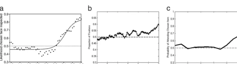
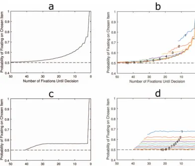
The LOB describes the finding that in the final moments before decision, individuals are far more likely to be looking at the item they are about to choose (Shimojo et al., 2003). When this looking bias is plotted against time it is shown to increase slowly at first, beginning approximately one sec-ond before the decision, but then rising rapidly until the moment the response is made, or very slightly before (see Figure 1). Crucially, experi-ments have shown that this is reflective of the underlying deliberation process (Krajbich et al., 2012; Shimojo et al., 2003; Simion & Shimojo, 2007). The cascade continues even when the vi-sual display turns blank, suggesting that shifts in visual attention reflect covert shifts in the item currently being considered (Simion & Shimojo, 2007). Furthermore, individuals are not merely attending to an object as part of planning the response action, for example, looking left to aid in pressing the left button. Nor are they simply halt-ing visual search while they make the requisite motor response. We know this because the cas-cade is still present when participants are forced to look away from the pictures in order to make their response (Glaholt & Reingold, 2009) and the final fixation on an item is often shorter than those preceding it, suggesting it is interrupted by a de-cision threshold being crossed (Krajbich et al.,

Figure 1. Empirically measured late onset bias during (a) preferential binary choice between faces (Shimojo et al., 2003); (b) multiattribute choice between 2 apartments each with 5 numerical attributes (Mullett and Tunney, 2016), and (c) choices between two risky gambles

(Stewart, Hermans, & Matthews, 2015). Note that whereas a and b are plotted against time,

c is plotted by discrete fixations.

2010). In addition, the characteristics of the LOB react and change subtly depending on the specific task with the cascade beginning earlier when there are more alternatives and the choice is more com-plex (Glaholt & Reingold, 2009;Glaholt, Wu, & Reingold, 2010; Schotter, Berry, McKenzie, & Rayner, 2010;Schotter, Gerety, & Rayner, 2012). This is evident inFigure 1, where panel a comes from a simple binary choice experiment, panel b comes from a complex multiattribute decision, and panel c comes from a risky gambles experi-ment. Although the three plots have differences, the LOB has some stable characteristics. It is characterized by attention being split equally be-tween items in the early and middle portions of the trial, before rising during the last moments before decision and finishing with a bias to be looking at the chosen item 60 –90% of the time, depending on choice complexity. Furthermore, although it is not often reported, in our own studies we have found that the LOB onsets at the same point prior to decision, regardless of how much time an indi-vidual has spent deliberating the choice before-hand. That is, trials with different RTs show the same absolute duration LOB.

One of the aims of this study is to examine competing explanations for the LOB. One prominent explanation is a feedback loop be-tween attention and evidence accumulation. In-dividuals are biased to pay more attention to rewarding items. Therefore, as one item begins to be preferred, there is a bias to fixate on it more, which in turn increases the probability of accumulating evidence in its favor (Glöckner & Betsch, 2008;Glöckner & Herbold, 2011; Shi-mojo et al., 2003). This explains findings that the cascade is larger when individuals are se-lecting the option they like, as opposed to dis-like (Mitsuda & Glaholt, 2014;Simion & Shi-mojo, 2006). However, others have suggested that the bias in looking can be better explained by the relevance of the evidence to the choice. In “like” tasks, individuals focus more on the positive information whereas in “dislike” tasks they do the opposite (Armel et al., 2008;Meloy & Russo, 2004; Schotter et al., 2010). More recent evidence suggests that early in delibera-tion attendelibera-tion is biased toward the more reward-ing stimuli, regardless of the current task, sug-gesting a bottom up effect on attention; then, a top-down system exerts more control as delib-eration continues, with attention being biased toward the item containing evidence most

rele-vant to the current decision task (Kovach, Sut-terer, Rushia, Teriakidis, & Jenison, 2014;

Schotter et al., 2012). In the case of reject tasks, attention becomes biased toward negative op-tions and the gaze cascade is still toward the item which is selected as the worst. Given the nuances and complexity of the arguments about whether positive evidence is always lated or whether negative evidence is accumu-lated in reject tasks as well as effects of bottom up and top down control, we focus here on the highly robust effects seen in preferential choices between positive items. Thus we do not address what characteristics may be driving the loop but focus on the more fundamental question of whether any kind of loop is required, or indeed capable, of producing the LOB.

The competing explanation for the cascade effect is that there is no loop, and no exogenous effects on attention (Krajbich & Rangel, 2011), with the exception of ignoring eliminated op-tions (Glaholt & Reingold, 2009;Glaholt et al., 2010). Instead, attention is allocated randomly and the cascade emerges because of a funda-mental property of the decision making process. This interpretation posits only that individuals are biased to accumulating evidence in favor of the currently attended item. Each item has its own accumulator, which is incremented as more evidence is acquired and a decision is only made once a threshold is reached thereby satis-fying a stopping rule. The LOB is predicted because evidence is accumulated more rapidly for the attended item. Therefore, when the threshold is reached and a response made, it is more likely that it is the currently attended item which has just accumulated the requisite evi-dence. By plotting attention locked to the point at which a decision is made, one is retrospec-tively plotting this antecedent shift in attention and the resulting increased accumulation rates which caused the choice to be made.

it increments that particular item’s accumulator. A decision is made when one item has accumulated enough evidence to be far enough ahead of the other. That is, a decision is made when the differ-encebetween accumulators reaches a set thresh-old. When there are more than two alternatives then one must start making additional assumptions about the relativistic comparison (e.g., highest ac-cumulator vs. 2nd highest, or highest vs. average). This particular debate is beyond the scope of this review because we deliberately focus only on bi-nary decisions (for a discussion seeKrajbich & Rangel, 2011;Teodorescu & Usher, 2013).

In absolute threshold models, each item has its own accumulator. However, a decision is made when any one accumulator reaches a set threshold, regardless of the state of the competing accumu-lator. Arguably there is more variation between the many models which employ an absolute stop-ping rule. These models often posit differing types of interaction and inhibition between the accumu-lators or inputs during evidence accumulation (see

Teodorescu & Usher, 2013, for a review). We take the most common assumptions and functional forms, then examine their fundamental properties in relation to the visual phenomena we are mod-eling. Toward the end of the article we also apply a very general approach which aims to identify whether particular assumptions could ever pro-duce these phenomena.

The simplest absolute threshold model exam-ined here is the independent race model, where there is no interaction and the accumulators simply race toward the threshold (Vickers, 1970). Although useful for illustrating simple effects, this model is rarely used in choice fit-ting as it is poor at predicfit-ting RT patterns. The first alternative tested is an assumption of mu-tual inhibition (Usher & McClelland, 2001). This describes a model where the total evidence accumulated for an option inhibits the input to competing accumulators. As one accumulator gets close to the decision threshold it is inhib-iting the accumulation of new evidence for other items, meaning it is able to increase its lead even more quickly. This could be a poten-tial explanation for a LOB. Another possible assumption is that of feedforward inhibition (Krajbich et al., 2010;Mazurek, Roitman, Dit-terich, & Shadlen, 2003; Niwa & Ditterich, 2008;Shadlen & Newsome, 1996). In feedfor-ward inhibition, the inputs to each accumulator have an excitatory effect on their own

accumu-lator, but an equal or proportional inhibitory effect on competing accumulators. This is math-ematically equivalent to normalizing the values at the input stage. Interestingly for this study, in binary choices a model with full inhibition is mathematically equivalent to a relative thresh-old model. The relativity is simply implemented at the evidence accumulation stage rather than the decision threshold stage: With complete in-hibition, differences are accumulated directly. Therefore the simple relativistic rule imple-mented here can also be represented as a special case of the feed-forward absolute threshold rule, where inhibition is 1 and decay is 0.

There are several sections to this article, each with its own purpose. To begin we use simple toy models whereby each simulated fixation results in a one unit increment of evidence. These simplified models are included to more clearly demonstrate the effects of differing assumptions. In the first section we demonstrate that a simple absolute model is unable to produce the LOB and demon-strate the reason for this. We then show that a very simple relative model is able to produce a LOB even when attention allocation is entirely random. The second section shows that the results remain the same when there is only a probabilistic link between attention and evidence accumulation. In the third section, we demonstrate the effect of adding a feedback loop as suggested by several visual attention models, which actually makes the model predictions worse. The fourth section ad-dresses different inhibition assumptions within the absolute threshold model. It is shown that a simple mutual inhibition model cannot predict the LOB and that the feedforward model can produce sim-ilar results to the relative threshold model, but only when inhibition is near 100%.

Finally, we present a large scale grid search of parameter space for a relative threshold model, a mutual inhibition model, and a feed-forward inhibition model (see Table 1). The relative threshold model is able to predict si-multaneously the qualitative characteristics of the LOB and many common properties of mea-sured RT distributions with a single set of pa-rameters. For the mutual inhibition model, we find parameter values which can predict the LOB but also result in unrealistic RT distribu-tions and we find values which can predict RT distributions, but fail to produce the LOB. There is no parameter set which can simultaneously predict both. We find similar results for the

feedforward inhibition model, with no single set of parameter values which can predict the LOB and RT distributions simultaneously. This model in particular we find to be very sensitive to small changes in parameter values, especially the level of inhibition.

Simulations

Absolute Threshold Models

The first model reported is that using a simple absolute threshold with attention having a de-terministic effect on evidence accumulation. This simple absolute stopping model is no lon-ger a serious candidate in the literature. Current absolute stopping models also incorporate inhi-bition between accumulators or inputs or both, and decay or leakage, and trial-to-trial variation in parameters. These additions are necessary to capture key results in choice and RT data. We start with this model, however, to illustrate the basic problem in producing a LOB. Below we show that incorporating the additional mecha-nisms listed above does not allow the models to capture simultaneously the LOB and even just basic properties of the RT distribution.

The model assumes that for each fixation, the attended item has its accumulator incremented by 1. To set the threshold we used a grid search to find the parameter that gives a RT closest to 16 fixations. We simulated 100,000 choices and the LOB was plotted by calculating the propor-tion of simulated choices where the preferred

item was fixated at each time point, working back from the moment the decision was made.

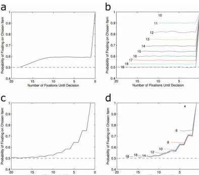
Figure 2ashows that this model fails to produce the classic LOB. Instead of a cascade there was a bias toward the chosen item which appears to develop gradually from the beginning of the choice, then plateaus early on. There is then a sudden tick up for the very last fixation, with 100% of trials ending while the preferred item is fixated. The latter is easily explained: because evidence can only be accumulated for the fix-ated item the accumulator can only be incre-mented to cross the decision threshold while the ultimately chosen item is being attended.

The cause of the long-term bias throughout the choice is less obvious. To see why this occurs it is helpful to plot the pattern of the LOB for choices with different RTs (Figure 2b). This reveals that for any choice with a given RT, the probability of having fixated on the chosen item is constant throughout. Consider a trial where a response is made after only 10 pieces of information have been collected. In this case there were exactly 10 fixations and since an accumulator has reached the decision threshold all 10 must necessarily have been toward that one item. Therefore there was a 100% chance for each fixation to have been di-rected to the chosen item. For a choice where exactly 11 pieces of evidence were accumulated, one knows that 10 of these must have been di-rected toward the chosen item. One also knows that, because of the deterministic nature of the model, the final fixation must have been directed Table 1

Summary of the Models Estimated Using Parameter Grid Search

Model Decision criterion Inhibition Decay

Free parameters

Absolute threshold (independent race model)

Evidence for 1 or evidence for 2 is greater than threshold

NA NA 2

Relative threshold Difference between evidence for 1 and evidence for 2 is greater than threshold

NA NA 2

Absolute threshold with feed forward inhibition

Evidence for 1 or evidence for 2 is greater than threshold

Input to each accumulator inhibits the input to competitors

Accumulated evidence decays as a proportion of total accumulated

4

Absolute threshold with mutual inhibition

Evidence for 1 or evidence for 2 is greater than threshold

Total evidence accumulated for an option inhibits the input to competitor

Accumulated evidence decays as a proportion of total accumulated

toward the chosen item. Therefore, for the first 10 fixations there is a 90% chance that an individual fixation was toward the chosen item. However, what is important for the failure to produce a LOB is that the order in which the evidence was accu-mulated is irrelevant to the choice. It is not spec-ified exactly when within the first 10 fixations attention was directed to the now chosen option. Only the last fixation is determined, hence the plateau followed by the sudden tick to 1.

Figure 2balso makes clear that the reason for the gradual rise in gaze bias at the start of the trial is simply because of averaging over different lengths of trials. Trials with longer RTs necessar-ily involve more fixations toward the nonchosen item and are included in the averaged LOB before

the shorter RT trials have even begun. As one moves closer to the decision point, trials with short RTs and much larger biases begin to be included in the average. This is why the bias plateaus 10 fixations before the decision.

Relative Threshold Models

Now we turn to models which assume that decisions are made using a relative stopping rule: instead of stopping when either item reaches a set threshold, the decision depends on the size of the difference between evidence ac-cumulated for either item. As this model uses a different decision rule, one cannot use the same threshold value as in the absolute threshold— Figure 2. Average LOB for absolute threshold model (a) and relative threshold model (c).

Also, shown are the patterns of LOB broken down by length of deliberation time (RTs) for absolute (b) and relative (d). See the online article for the color version of this figure.

after all a value of 5 for the threshold, for example, would be the difference in evidence for a relative stopping rule but would be the total evidence for one accumulator in an abso-lute stopping rule. A grid search was again used to identify a difference threshold of 4 as pro-viding a mean RT closest to 16. The model simulated 100,000 choices and the LOB was plotted by averaging attention over all choices.

Figure 2c shows that the pattern matches the classic LOB finding. The probability of fixating the chosen item increases with a convex shape just prior to the decision being made.

The LOB was then plotted for trials of dif-ferent RTs. Unlike the absolute threshold rule, the relative rule could potentially produce infi-nitely long RTs as a result of random walk dynamics. However, the probability of observ-ing longer RTs drops quickly and they are rare in these simulations. To allow for this we only plot discrete RTs which occurred in at least 5% of simulated choices.

Figure 2dshows that the LOB develops with a very similar time course for all RTs. There was a slight early bias evident in very short trials which deviates from the average cascade. However, this was much too small to be driving the overall effect and quickly converges to match the fixation biases of other RTs. Cru-cially, a pattern of increasing bias was found as the decision point approaches, regardless of the trial’s RT. This is because creating a relative difference between the accumulators requires a sequential series of fixations on one item and a decision will be reached at the end of this run. So unlike the absolute threshold rule, there is a constraint on the order in which evidence is accumulated leading up to a response.

Nondeterministic Evidence Accumulation

One may think it possible that these results are attributable to the improbable assumption of a deterministic rule linking fixations to evidence accumulation. Indeed models of evidence accu-mulation generally predict only a probabilistic bias toward accumulating evidence for the at-tended item (Krajbich et al., 2010). To address this, both the absolute and relative threshold models were run again, but this time fixating on an item resulted in a 65% chance of increment-ing the accumulator for the attended item. In the other 35% of cases, evidence was accumulated

for the unattended item instead. The bias of 65% was chosen to approximately match the bias that attention has on evidence accumula-tion as has been estimated in empirical studies (Krajbich et al., 2010).Figure 3shows that the pattern of results is virtually identical. The only difference for the absolute threshold model is that the size of the early bias has been reduced and the final tick only represents 65% of trials where the final fixation is on the chosen item. The probabilistic rule means that the overall bias effect cannot be more than 65% but it does not change the underlying reason for the lack of LOB: the order in which evidence is accumu-lated does not matter in the absolute threshold model. For the relative threshold, the results still show a cascade of increasing bias toward the chosen item before decision but now the cas-cade has a maximum bias of 65%.

Biases in Attention Allocation

One common interpretation of the LOB is that attention is biased toward the currently favored item, creating a positive feedback loop. Essentially, as more evidence is accumulated for an item it is more likely to be attended, thus producing the LOB in the final moments before choice when evidence is highest. This is inter-esting as it is intuitively plausible that an abso-lute threshold rule could produce the LOB when combined with attentional bias. Therefore the modeling approach is applied to test this intu-ition. The only difference from the absolute threshold model described in the above model is in the allocation of attention. In the previous model this was entirely random and indepen-dent of previous fixation locations. In this model the following equation was used:

ProbAttenleft⫽

Eleft⫹b

Eleft⫹b⫹Eright⫹b

(1)

directed toward the right. The value of b⫽ 3 was used to produce the reported results, how-ever there is no qualitative change when b is given very high values.

Figure 4 shows that even with a substantial attention bias, the absolute threshold decision model is not able to produce the LOB. When attention bias is plotted separately for different RTs, there is a clear increase in the probability of attending the chosen item. However, this occurs early on and the effect is still very dependent on the RT itself. Where there is a long RT, the fixa-tions must necessarily have been split relatively equally between the items. Therefore there was never a large difference between the evidence

accumulated, meaning there was also never a large attention bias toward either.

Inhibition

A number of accumulator models incorporate inhibition, whereby the rate of evidence accu-mulation for any option is directly affected by the other items available. This is especially rel-evant here because depending on the specific implementation of inhibition, these models can be mathematically identical to relative threshold models when predicting choice and RTs. That is, when modeling choice and RTs in a two alternative decision, they will make identical Figure 3. Average LOB for absolute threshold model (a) and relative threshold model (c)

when attention is modeled as having a probabilistic bias on evidence accumulation. The results show no qualitative differences compared to the deterministic rule, even when the patterns of LOB are separated by RTs for both absolute (b) and relative (d). Note the change in scale fromFigure 2. See the online article for the color version of this figure.

predictions. In this section we explore how at-tention effects can differentiate between them.

A number of models, including leaky com-peting accumulators (Usher & McClelland, 2001), assume the inhibition of evidence accu-mulation is dependent on the total evidence accumulated for the competing option. That is, if one option has accumulated so much evidence that it is close to reaching the decision thresh-old, it will almost entirely inhibit the accumu-lation of evidence for the competing option. To simulate this pattern of accumulation, attention is randomly allocated on each time step. When attention is directed at item 1 we implement evidence accumulation using:

⌬E₁⫽AV₁⫺(1⫺A)IE2 T

⌬E2⫽(1⫺A)V2⫺

AIE₁ T

(2)

where ⌬Ei is the change in accumulated evi-dence for item i,Ei is the total evidence accu-mulated, and V is the value input from the stimulus.Ais the attention bias toward accumu-lating evidence for the attended item, I is the inhibition parameter, and T is the decision threshold. This normalization by the threshold means that if I⫽ 1, when one item has accu-mulated enough evidence to be half way to the decision threshold, the input to the competing

item is reduced by 50%. As the simulation uses the same absolute threshold rule as the previous models the same parameters are applied. To demonstrate the qualitative effect of inhibition most clearly, the parameterIis set to 1.

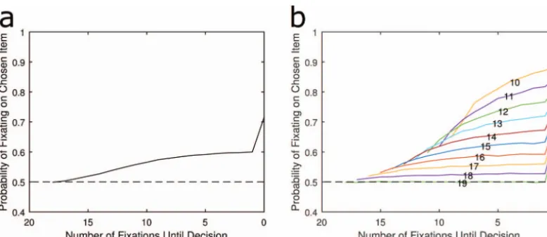
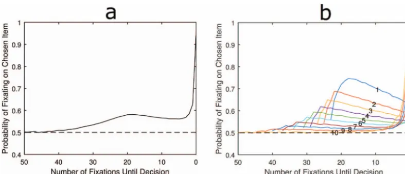
Figure 5a shows that the resulting LOB shows a very early rise from chance, followed by a decline before a rapid rise for the last few fixations. The reason for this pattern becomes clear when the plots are split by RT.Figure 5b

⌬E1⫽AV1⫺(1⫺A)IV2

⌬E2⫽(1⫺A)V2⫺AIV1

(3)

This model has the interesting property that when inhibition is equal to 1, it becomes math-ematically equivalent to a relative threshold model without inhibition. However, the relativ-ity enters the model at the point of evidence accumulation, instead of later, at the decision rule. Our first aim here is to establish whether both assumptions are able to predict the LOB. Because of this functional similarity, the same threshold value of 4 was initially used, however due to the inhibition term reducing the amount of evidence accumulated on each fixation RTs were implausibly long. A threshold of 2 is in-stead used, though the qualitative results remain the same.

Figure 6ashows that when inhibition is set to 1, the model produces the desired pattern of a monotonically rising bias immediately before choice. Figure 6b shows that some of this is caused or accentuated by shorter RT trials hav-ing a higher bias overall. However, this effect is very different to that found in other absolute threshold models because in all cases the bias increases over the final few fixations rather than being flat and then showing a sudden spike.

Next we examine what happens to the LOB when inhibition is not equal to one, thus break-ing the equivalence to relative threshold mod-els. The reason for this is that empirical fitting

of behavioral data rarely yields such high esti-mates of inhibition. Therefore, an additional simulation was performed with inhibition re-duced to 0.5. Figure 6c shows that the gaze cascade now looks nearly identical to that pro-duced by the corresponding model with no in-hibition at all.

The reason for this large change in the LOB with partial rather than complete inhibition is as follows. With complete inhibition (I ⫽ 1), the attended and unattended items have their accu-mulators increased and decreased respectively by the same amount (in this simulation, by ⫹ 0.3 and ⫺0.3). This is analogous to a single item accumulating 0.6 in a relative threshold rule because the total evidence accumulated at any time is zero. However, with partial inhibi-tion (I⫽0.5) the attended item is increased by 0.48 and the unattended is also increased but only by 0.03. Therefore, the model is no longer equivalent to that of the relative threshold and because the gain of attending an item is greater than the penalty of attending its competitor, the resulting LOB is similar to that of other absolute threshold models. The plateau pattern is still evident even when I is large enough for the unattended item to experience negative accu-mulation, just so long as this is smaller than the positive gain associated with being attended. In fact Figure B1 in the Appendix B shows that even when I⫽0.9 there is notable flattening in the LOB for separate RT trials and when I⫽0.8 Figure 5. Average LOB for absolute threshold model with mutual inhibition (a) and the

LOBs from the same model when simulations are split into deciles by RT. See the online article for the color version of this figure.

the plateau pattern is obvious in the overall LOB.

Real Time Simulation and Model Tests

The simplified assumption of each fixation resulting in a single quantum of evidence being accumulated is useful for illustrating the effects of differing RTs. However, the majority of drift diffusion models posit that evidence is accumu-lated continuously over time and that the accu-mulation of evidence at each timepoint is biased toward the item which happens to be currently fixated (Busemeyer & Townsend, 1993; Kra-jbich et al., 2010; Krajbich & Rangel, 2011).

Furthermore, in the models presented up until this point we have deliberately manipulated as few parameters as possible so that we can more easily identify the effect of individual model properties. However, nearly all models of choice are fitted with several estimated param-eters, all of which can interact and may combine to produce the LOB and RT patterns common in choice data. The following modeling addresses both of these issues. First, we assume that evi-dence is accumulated constantly and over a series of fixations with varying durations. Sec-ond, we perform a large scale grid search of the parameter space to test what proportion of the Figure 6. The average LOB for an absolute threshold rule with feedforward inhibition when

potential parameters can predict properties of the LOB and predict RT distributions that match those commonly found in empirical studies.

To approximate continuous evidence accu-mulation the time during deliberation was split into bins of 10ms. At the start of each choice, a fixation duration was sampled from the distri-bution measured inMullett and Tunney (2016; SeeFigure A1inAppendix Afor the distribu-tion of sampled fixadistribu-tion duradistribu-tions). Attendistribu-tion was randomly assigned to one of the items and evi-dence was sampled with an attentional bias for the duration of the randomly sampled fixation. At the end of this fixation a new duration was sampled and attention was again randomly assigned.

We begin with a relative threshold model. The parameters that are allowed to vary are the attention bias,A, and the decision threshold,T. The minimum value forAis set at 0.5, as this value results in no bias to either option. A value of less than 0.5 would lead to a bias toward the unattended item. Thirty potential values of A

were examined, each of which were spaced linearly between 0.5 and 1. For the threshold value there is no upper bound therefore a max-imum was selected that would explore the ex-tremes of the model’s range. We selected a minimum of 2 and a maximum of 100. Again, 30 values were selected, equally spaced be-tween. This resulted in 900 combinations, each of which were simulated for 33,000 choices. (33,000 choices is the maximum given the large computer memory burden of storing the entire sequence for every simulation.) To enable com-putational tractability and keep these simula-tions within the capacity of our equipment, the simulation would terminate once the simulated RT was more than 30 seconds. If a decision had not been reached then a null response was re-corded.

The large number of parameter combinations means it is not possible to discuss them indi-vidually. Therefore we implement a number of qualitative checks on the predicted LOBs and RT distributions. These enable us to specify characteristics which are present in individuals’ behavior and then objectively test which param-eter sets and which models satisfy them. These can then be used to partition the parameter space and report the volume of parameter space in which our criteria are met (Lee & Corlett, 2003;Pitt, Kim, Navarro, & Myung, 2006). In total we use five criteria listed inTable 2.

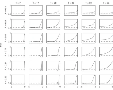
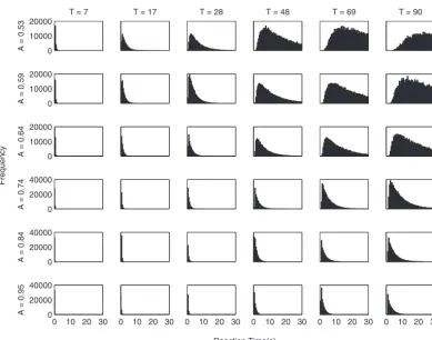
Simulating the relative threshold model shows that there are parameter combinations which sat-isfy all five of these criteria simultaneously (see the first column ofTable 3). These are in a small minority, but the fact that these values are found demonstrates that the underlying properties of this two parameter relative threshold model allow it to simultaneously fit the behavior observed in visual attention and choice experiments.Figure 7shows the gaze cascades produced by a small but repre-sentative sample of the parameter space, and Fig-ure 8 shows the corresponding distributions of RTs. The observable effects are all quite intuitive. A higher threshold means that responses take lon-ger and the gaze cascade becomes more stretched over time as a longer run of samples is required for an item to reach the higher threshold. Increasing the attention bias serves to shorten RTs as each increment of information has a larger effect. It also increases the magnitude of the bias, but not in a linear manner because of the properties of a biased random walk.

Absolute Threshold and Mutual Inhibition

We now turn to models with an absolute stopping rule, beginning with one that

imple-Table 2

Criteria Used to Test Each Model’s Performance

Criteria

Tests behavioral or visual phenomena

The attention bias at the time of response is between .6 and .9 Visual The average bias from the start of the choice until 2 seconds before response is between

.45 and .55 Visual

The mean RT is between 2 and 8 seconds Behavioral

The skewness of the RT distribution is positive and greater than 1 Behavioral No more than 1% of choices where the model fails to make a response within 30 seconds Behavioral

ments mutual inhibition. For these absolute threshold models we allow more free parame-ters to vary and test a very large number of combinations. This added complexity allows us to better represent the general properties of

ab-solute threshold models commonly fitted to be-havioral data. In total we vary four parameters: attention bias A, the decision threshold T, the decay rated, and the inhibition parameterI. The decay rate is implemented at the beginning of each time point using:

Et⫽Et_⫺1

冉

t

冊

This equation means that whend⫽1 evidence decays at a rate equal to the maximum rate which it can be accumulated. Whend⫽0, there is no decay at all and perfect responding would be possible, given enough time. Once the decay rate has been applied, evidence accumulation is calculated usingEquation 2.

Table 3

Proportion of Parameter Space Which Satisfies Different Numbers of Criteria for Each Model Type

Number of criteria satisfied

Relative threshold

Mutual inhibition

Feed forward inhibition

5 2% 0% 0%

4 27% 1% 1%

3 35% 6% 3%

2 26% 15% 16%

1 10% 61% 66%

0 0% 17% 14%

0.5 1

T = 7

A = 0.53

T = 17 T = 28 T = 48 T = 69 T = 90

0.5 1

A = 0.59

0.5 1

A = 0.64

0.5 1

Bias

A = 0.74

0.5 1

A = 0.84

0 5

0.5 1

A = 0.95

0

5 5 0

Time to decision (s) 0

5 5 0 5 0

The parametersdandIare all bounded by 0 and 1. Ten equally spaced values were tested, with these bounds used as the maximum and minimum values. For A, we used the same bounds as in the relative threshold model and tested 10 equally spaced values between. The parameter T again has no upper bound and as demonstrated earlier the threshold in an abso-lute model must generally be higher than in the relative threshold model, meaning a large value could be plausible. Simultaneously, the interac-tion with decay and inhibiinterac-tion will mean that for certain parameter configurations a very low threshold could be plausible. To cover these extremes we always included very small values ofT: 1, 3, and 5. We then set our maximum to 320 and selected 10 evenly spaced values be-tween 10 and 320. This resulted in 13,000 com-binations of parameter values and, as in the relative threshold model, 33,000 choices were simulated for each.

As the second column inTable 3shows, none of the 13,000 tested combinations were able to simultaneously satisfy all 5 criteria, though a small number were able to satisfy 4. It is not possible to simultaneously show the effect of varying all 4 parameters so instead we present a series of plots for each parameter. The values of three out of four parameters are kept constant and the plots show the cascade and RT distri-bution for each tested level of the remaining one. The values of the remaining three param-eters are selected to present results that perform well, but their primary purpose is to demon-strate the effect of varying the parameter of interest. In all cases we seek to present the clearest possible demonstration of the effect of changing the parameter of interest.

InFigure 9the top two rows show the effect of changing the threshold whenI⫽1 and the bottom two rows show the same effect when I ⫽ 0. WhereI ⫽ 1 we see the same pattern as in the 0

10000 20000

A = 0.53

T = 7 T = 17 T = 28 T = 48 T = 69 T = 90

0 10000 20000

A = 0.59

0 10000 20000

A = 0.64

0 20000 40000

Frequency

A = 0.74

0 20000 40000

A = 0.84

0 10 20 30

0 20000 40000

A = 0.95

0 10 20 30 0 10 20 30

Reaction Time(s)

0 10 20 30 0 10 20 30 0 10 20 30

Figure 8. The RT distributions estimated by the grid search of parameters for the relative threshold rule. Columns list different values for the thresholdT, and rows correspond to values of attention biasA.

simple example ofFigure 5a, where the cascade initially rises and then falls, before a tick up at the end. This increase at the end matches many prop-erties of the LOB, but the model fails because of the large bias preceding it. The threshold increase stretches this out over time, but it is always pres-ent. WhenI⫽0 the model can perform reason-ably well by incorporating decay. This produces good RT distributions and a rise in the final mo-ments, without a preceding bias. However, the

model fails because the scale of the decay rate required to produce the RT distribution results in 100% of attention being directed toward the cho-sen item. In many cases, it reaches 100% before the end. In addition the increasing threshold stretches the LOB to form a gradual rise.

InFigure 10decay is varied. When decay is 0, RTs are all very short and the LOB shows an early rise, then plateau and final sudden tick up. This becomes smoothed as decay is increased, but at Figure 9. The top row of panels shows the average LOB produced by increasing the

threshold parameter in a model with full mutual inhibition. The second row shows the RT distributions for the same models. The lower two rows show the effect of increasing the threshold parameter when inhibition is set to zero.

the same time the duration of the LOB is extended and onsets earlier than is seen in eyetracking ev-idence. In addition, 100% of attention must be allocated to the chosen item for some time before choice so that evidence accumulation overcomes the rate of decay. For very high levels of decay the model fails to reach threshold in nearly all choices meaning results cannot be plotted.

Figure 11shows that increasing the size of the attention bias while keeping all other parameters constant reduces RT time as the difference in evidence accumulated for either item at each step is larger. It also increases the size of the bias at the point where a decision is made.

Figure 12 displays the effect of increasing inhibition. This serves to increase RT and allows the model to produce positively skewed distribu-tions. However, an early bias toward attending the chosen item is seen at all levels ofI.

Absolute Threshold and Feedforward Inhibition

When fitting an absolute threshold model with feedforward inhibition we use the same parameter values as used for fitting the mutual inhibition model. Evidence decay was also implemented in the same manner. However, evidence accumula-tion was estimated usingequation 3. Again,Table 3 shows that no parameter values were found which satisfied all 5 criteria.Table 4shows that the criteria the model particularly struggles with is the size of the bias in the final moments. To show the reasons for this we plot the effect of changing each parameter value as was done for the mutual inhibition model.

Figure 13shows that increasing the threshold increases the average RT, but when the model contains both decay and inhibition the

distribu-tion of RTs does not become more positively skewed. The LOB also becomes more elon-gated, but even with relatively high inhibition and some decay, the model still produces an early bias toward the chosen item.

Figure 14shows that increasing the decay has a large and pronounced effect. At higher levels the decay interacts with inhibition so that no choices are completed, even at low thresholds. High decay rates can also result in attention becoming biased toward the competing item before a sudden up-ward tick marking the onset of the LOB. This is because the high decay rate combines with the inhibition to mean there is an almost lexicographic and deterministic rule of a decision being made afterXsamples in a row. Thus for a choice to take longer than that number of samples attention must necessarily have been directed to the other item immediately prior to that run. At lower levels of decay the LOB onsets early and results in a grad-ual rise as well as showing a slight plateau at very low levels, even though inhibition is relatively high.

When attention bias is low, RTs are all rela-tively similar because the random allocation of attention is introducing less variability into the model.Figure 15shows that even with a midrange value for inhibition there is an early bias and no positive skew in RTs. At higher levels the rela-tionship becomes more deterministic. Although the LOB onsets much closer to the end of the choice there is still slight early bias and the bias at the time of choice is 100%.

Figure 16shows that increasing the inhibition parameter improves the model’s ability to produce positively skewed RTs with distributions which match behavioral data. However, this also in-creases the size of the attention bias at the final Figure 11. The LOB and RT distributions produced by different levels of attention bias

within a mutual inhibition model.

moment before choice and the resulting predic-tions are much more extreme than is observed in subjects’ responses. Overall these results show that although there is likely to be a parameter set where the model can match all of these values, the region of parameter space where inhibition, decay and attention bias are balanced is very small. The variance in parameter values estimated from ex-isting choice and RT data is larger by at least an order of magnitude.

Discussion

Simulations of choice times and attention allo-cation from evidence accumulation models with relative and absolute stopping rules have revealed two clear results. First, the simulations show that it is possible for a model of decision making to predict the LOB effect without any modulation of attention or feedback loop. Such a loop may still exist, but clearly it is not necessary and in some models including it can actually worsen the mo-del’s performance. Second, we show that an evi-dence accumulation model with a relative

stop-ping rule can predict the qualitative patterns of the LOB and RT distributions commonly found in empirical data. It does so even when implemented in the most simple form possible, with no decay or inhibition. Models with an absolute stopping rule struggle to explain these effects even with addi-tional assumptions and free parameters. The re-sults of simple simulations show that a model with mutual inhibition fails to produce the LOB, whereas feedforward inhibition can only do so when the inhibition is near 1, something not ob-served in fits to choice and RT data. A large scale grid search simulating real-time evidence accumu-lation shows that a relative threshold rule can satisfy qualitative tests for the LOB and RT dis-tributions with a single set of parameters. Con-versely we find no parameter sets which can do so for the absolute threshold model with either mu-tual or feedforward inhibition. The manner in which multiple parameters interact with each other suggests that a set of values does exist for feedforward inhibition given a grid search with very high resolution, particularly when one con-siders that the relative threshold rule is held as a special case within the absolute threshold model with feed-forward inhibition. However, the area of parameter space is small; much smaller than the variance generally reported when fitting parame-ters to behavioral data alone.

Collapsing or Stationary Boundaries

One possibility that we do not directly test is that of collapsing boundaries. This assumption is included in a number of relative threshold mod-els because when evidence for each alternative is equal, then relative threshold rules can predict unrealistically long RTs or fail to converge on a choice at all. Collapsing boundaries address this Table 4

Proportion of Parameter Space Which Satisfies Each of the Five Model Criteria

Criteria

Relative threshold

Mutual inhibition

Feed forward inhibition

End bias .6–.9 20% 4% 3%

Early stage bias .45–.55 85% 21% 23%

Mean RT 2–8s 35% 21% 15%

Positive skew in RT

distribution 77% 18% 12% 99% of decisions made

in 30s 66% 48% 57%

problem. We do not examine this subclass of models here because we show that even the sim-plest relative threshold model produces a robust LOB before this additional assumption is in-cluded. What is particularly interesting though is that a collapsing boundary can make a relative threshold rule equivalent to an absolute threshold rule when predicting choice and RT (Zhang, Lee, Vandekerckhove, Maris, & Wagenmakers, 2014). This does not qualitatively change our conclu-sions, as it of course does not affect the predictions of the absolute threshold model, while it simply adds more degrees of freedom to the relative threshold model. However, it means the LOB could be used to test for the presence of collapsing boundaries in future work: a relative threshold rule with collapsing boundaries would predict a differ-ent pattern of LOB at differdiffer-ent RTs. This is attrib-utable to changes in the relative impact of the accumulation process (which is weighted by at-tention), and the rate at which the boundary col-lapses (which is attention agnostic) as deliberation time increases. This effect can also be used in

future development of such models to estimate the rate at which a boundary may collapse while si-multaneously estimating, and controlling for, the biasing effect of attention.

Feedback Loop or Patterns Emerging From Random Attention?

The reason that the relative threshold produces the LOB is that a decision is made after several consecutive incidences of evidence being accu-mulated for one item. By time locking the analysis to the point of response, it is necessarily true that evidence must have been accumulated for the chosen item in the immediately preceding mo-ments. If attention biases evidence accumulation, it must also be true that attention was more likely to be directed toward the chosen item in those immediately preceding moments. The apparent build-up of a bias immediately before a choice gives a powerful intuitive sense of causality: that a deliberate, nonrandom shift in attention causes the resulting decision. However, the results here dem-Figure 13. The LOB and RT distributions produced by different thresholds within a

feedforward inhibition model.

Figure 14. The LOB and RT distributions produced by different rates of decay within a feedforward inhibition model. Blank subplots occur for parameter values where too few decisions were made within the imposed deadline of 30s and therefore results cannot be plotted.

onstrate that because the analysis of attention is essentially retrospective, a truly random assign-ment of attention still predicts the LOB. In fact, assuming a direct loop between accumulated evi-dence and attention does not alter the models’ predictions. These results are consistent with many recent findings which do not require or assume any systematic bias in attention (Glaholt & Reingold, 2009;Glaholt et al., 2010;Krajbich et al., 2010,2012;Krajbich & Rangel, 2011; Mit-suda & Glaholt, 2014). They also support studies showing that the mere exposure effect does not require any volitional allocation of attention, and that it is possible for it to be controlled entirely by the environment and presentation duration of stimuli (Bird et al., 2012).

It seems unlikely that attention is entirely ran-dom, and several patterns have already been iden-tified (Shi et al., 2013). These include the ignoring of poor options, seemingly because they hit a lower boundary of evidence (Glaholt & Reingold, 2009) and modifying attention switching patterns between items and attributes depending on the stage of choice process (Shi et al., 2013). How-ever, these effects would not be relevant in binary

choice. An effect which could present an interest-ing alternative explanation is that rather than at-tention being directed more frequently toward the preferred item, attention lingers for longer every time a high value item is attended. Analysis of fixation and dwell durations has indeed shown that they are longer for preferred items, however this does not increase over the duration of the trial (Glaholt & Reingold, 2009,2011;Glaholt et al., 2010; Orquin & Mueller Loose, 2013). If any-thing, the effect is most pronounced in the first fixation and reduced during the rest of the trial. Therefore without an increase over time it cannot explain the LOB.

Stopping Rules and Inhibition in Evidence Accumulation Models

Evidence accumulation models using both rel-ative stopping rules and absolute stopping rules have been shown to fit RT and choice data well in different scenarios (Teodorescu & Usher, 2013). Some studies have also shown that an attention weighted relative threshold model can produce the LOB having been fitted to empirical data based Figure 15. The LOB and RT distributions produced by different levels of attention bias

within a feedforward inhibition model.

only on RTs and choices (Krajbich et al., 2010). However, this is the first attempt to model both relative threshold rules and absolute threshold rules and examine their fit to behavioral and visual phenomena simultaneously. The results of our grid search analyses show that the relative thresh-old rule can produce familiar RT distributions and LOB plots which match those from empirical da-ta. It is perhaps surprising that it is such a small proportion of the parameter space which can sat-isfy all of our qualitative tests simultaneously. However, asFigure 8shows, the RT distribution is always positively skewed and the LOB always shows a convex rise from a neutral early bias. The fact that the model can capture these qualitative patterns with nearly any viable parameter values shows that a more complex version incorporating inhibition, decay, or collapsing thresholds would find suitable parameter values with even more flexibility to fit behavioral data. In fact prior fits to eye tracking data have used additional assump-tions about inhibition (Krajbich et al., 2010).

For absolute threshold models both decay and inhibition were allowed to vary. This is because these parameters are crucial to the majority of absolute threshold models when fitting RT and choice data. Allowing only the threshold and at-tention bias to vary would result in us only testing the independent race model, which is now in-cluded as a special case when decay and inhibition are both 0. Within the literature on evidence ac-cumulation models there is debate about the point at which inhibition should enter the model, either as mutual inhibition of accumulated evidence or as accumulators inhibiting the input to other ac-cumulators in feed-forward inhibition. We use simple simulations to show that a mutual inhibi-tion assumpinhibi-tion, based on the total evidence ac-cumulated, fails to predict the LOB under basic assumptions. This is because if one item builds up a large lead the inhibition overwhelms the atten-tion bias, meaning it is less important which item is being attended to. A model with feedforward inhibition, where inhibition acts at the level of input, performs much better. It can mimic a rela-tive threshold model very closely when inhibition is 1, or at least very high. However, this breaks down quickly as the inhibition parameter is re-duced to more behaviorally plausible levels.

The large scale grid search shows that both inhibition assumptions can predict the LOB under some parameters and can predict realistic RT dis-tributions under others, but we find no overlap

where either model can predict both simultane-ously. The fact that the feed-forward model with complete inhibition is mathematically equivalent to the relative threshold models means that a grid search with sufficient resolution would find suit-able parameters. However, our analyses have shown that the LOB predictions are very sensitive to any reduction in inhibition away from its max-imum value of 1. Finding parameter sets for ab-solute threshold models at realistic levels of inhibition seems like a remote possibility. Further-more, if such a set were found, the proportion of parameter space occupied must be small as it must fit in between the nodes of the grid we explored. Given the scale of variance seen in parameter estimates from behavioral data, it would be in-credibly difficult to fit such a model to individuals’ responses.

References

Armel, K. C., Beaumel, A., & Rangel, A. (2008). Biasing simple choices by manipulating relative visual attention.Judgment and Decision Making, 3,396 – 403.

Atalay, A. S., Bodur, H. O., & Rasolofoarison, D. (2012). Shining in the center: Central gaze cascade effect on product choice. Journal of Consumer Research, 39,848 – 866.http://dx.doi.org/10.1086/ 665984

Bird, G. D., Lauwereyns, J., & Crawford, M. T. (2012). The role of eye movements in decision making and the prospect of exposure effects. Vi-sion Research, 60, 16 –21. http://dx.doi.org/10 .1016/j.visres.2012.02.014

Busemeyer, J. R., & Townsend, J. T. (1993). Deci-sion field theory: A dynamic-cognitive approach to decision making in an uncertain environment. Psy-chological Review, 100, 432– 459. http://dx.doi .org/10.1037/0033-295X.100.3.432

Fang, X., Singh, S., & Ahluwalia, R. (2007). An examination of different explanations for the mere exposure effect.Journal of Consumer Research, 34,97–103.http://dx.doi.org/10.1086/513050 Fiedler, S., & Glöckner, A. (2012). The dynamics of

decision making in risky choice: An eye-tracking analysis.Frontiers in Psychology, 3,335.http://dx .doi.org/10.3389/fpsyg.2012.00335

Glaholt, M. G., & Reingold, E. M. (2009). The time course of gaze bias in visual decision tasks.Visual Cognition, 17, 1228 –1243. http://dx.doi.org/10 .1080/13506280802362962

Glaholt, M. G., & Reingold, E. M. (2011). Eye move-ment monitoring as a process tracing methodology in decision making research.Journal of

ence, Psychology, and Economics, 4, 125–146. http://dx.doi.org/10.1037/a0020692

Glaholt, M. G., Wu, M.-C., & Reingold, E. M. (2010). Evidence for top-down control of eye movements dur-ing visual decision makdur-ing.Journal of Vision, 10,15. http://dx.doi.org/10.1167/10.5.15

Glöckner, A., & Betsch, T. (2008).Do people make decisions under risk based on ignorance? An em-pirical test of the priority heuristic against cumu-lative prospect theory. Bonn, Germany: Max Planck Institute for Research on Collective Goods. Glöckner, A., & Herbold, A.-K. (2011). An eye-tracking study on information processing in risky decisions: Evidence for compensatory strategies based on automatic processes. Journal of Behav-ioral Decision Making, 24, 71–98. http://dx.doi .org/10.1002/bdm.684

Kim, B. E., Seligman, D., & Kable, J. W. (2012). Preference reversals in decision making under risk are accompanied by changes in attention to differ-ent attributes.Frontiers in Neuroscience, 6,109. http://dx.doi.org/10.3389/fnins.2012.00109 Kovach, C. K., Sutterer, M. J., Rushia, S. N., Teriakidis,

A., & Jenison, R. L. (2014). Two systems drive atten-tion to rewards.Frontiers in Psychology, 5,46.http:// dx.doi.org/10.3389/fpsyg.2014.00046

Krajbich, I., Armel, C., & Rangel, A. (2010). Visual fixations and the computation and comparison of value in simple choice.Nature Neuroscience, 13, 1292–1298.http://dx.doi.org/10.1038/nn.2635 Krajbich, I., Lu, D., Camerer, C., & Rangel, A.

(2012). The attentional drift-diffusion model ex-tends to simple purchasing decisions.Frontiers in Psychology, 3, 193. http://dx.doi.org/10.3389/ fpsyg.2012.00193

Krajbich, I., & Rangel, A. (2011). Multialternative drift-diffusion model predicts the relationship be-tween visual fixations and choice in value-based decisions. PNAS Proceedings of the National Academy of Sciences of the United States of Amer-ica, 108, 13852–13857.http://dx.doi.org/10.1073/ pnas.1101328108

Lee, M. D., & Corlett, E. Y. (2003). Sequential sampling models of human text classification. Cognitive Science, 27,159 –193.http://dx.doi.org/ 10.1207/s15516709cog2702_2

Mandler, G., Nakamura, Y., & Van Zandt, B. J. (1987). Nonspecific effects of exposure on stimuli that cannot be recognized.Journal of Experimen-tal Psychology: Learning, Memory, and Cogni-tion, 13, 646 – 648. http://dx.doi.org/10.1037/ 0278-7393.13.4.646

Mazurek, M. E., Roitman, J. D., Ditterich, J., & Shadlen, M. N. (2003). A role for neural integra-tors in perceptual decision making.Cerebral Cor-tex, 13, 1257–1269. http://dx.doi.org/10.1093/ cercor/bhg097

Meloy, M. G., & Russo, J. E. (2004). Binary choice under instructions to select versus reject. Organi-zational Behavior and Human Decision Processes, 93, 114 –128. http://dx.doi.org/10.1016/j.obhdp .2003.12.002

Mitsuda, T., & Glaholt, M. G. (2014). Gaze bias during visual preference judgements: Effects of stimulus category and decision instructions.Visual Cognition, 22, 11–29. http://dx.doi.org/10.1080/ 13506285.2014.881447

Mullett, T. L., & Tunney, R. J. (2016).Visual atten-tion and attribute weighting in choice models. Manuscript submitted for publication.

Niwa, M., & Ditterich, J. (2008). Perceptual deci-sions between multiple directions of visual motion. The Journal of Neuroscience, 28, 4435– 4445. http://dx.doi.org/10.1523/JNEUROSCI.5564-07 .2008

Noguchi, T., & Stewart, N. (2014). In the attraction, compromise, and similarity effects, alternatives are repeatedly compared in pairs on single dimen-sions.Cognition, 132,44 –56.http://dx.doi.org/10 .1016/j.cognition.2014.03.006

Nordhielm, C. L. (2002). The influence of level of processing on advertising repetition effects. Jour-nal of Consumer Research, 29,371–382.http://dx .doi.org/10.1086/344428

Orquin, J. L., & Mueller Loose, S. (2013). Attention and choice: A review on eye movements in deci-sion making.Acta Psychologica, 144, 190 –206. http://dx.doi.org/10.1016/j.actpsy.2013.06.003 Pitt, M. A., Kim, W., Navarro, D. J., & Myung, J. I.

(2006). Global model analysis by parameter space partitioning. Psychological Review, 113, 57– 83. http://dx.doi.org/10.1037/0033-295X.113.1.57 Ratcliff, R., & McKoon, G. (2008). The diffusion

decision model: Theory and data for two-choice decision tasks.Neural Computation, 20,873–922. http://dx.doi.org/10.1162/neco.2008.12-06-420 Schotter, E. R., Berry, R. W., McKenzie, C. R. M., &

Rayner, K. (2010). Gaze bias: Selective encoding and liking effects.Visual Cognition, 18,1113–1132.http:// dx.doi.org/10.1080/13506281003668900

Schotter, E. R., Gerety, C., & Rayner, K. (2012). Heu-ristics and criterion setting during selective encoding in visual decision-making: Evidence from eye move-ments. Visual Cognition, 20,1110 –1129. http://dx .doi.org/10.1080/13506285.2012.735719

Shadlen, M. N., & Newsome, W. T. (1996). Motion perception: Seeing and deciding. PNAS Proceed-ings of the National Academy of Sciences of the United States of America, 93, 628 – 633.http://dx .doi.org/10.1073/pnas.93.2.628

Shimojo, S., Simion, C., Shimojo, E., & Scheier, C. (2003). Gaze bias both reflects and influences pref-erence.Nature Neuroscience, 6,1317–1322.http:// dx.doi.org/10.1038/nn1150

Simion, C., & Shimojo, S. (2006). Early interactions be-tween orienting, visual sampling and decision making in facial preference.Vision Research, 46,3331–3335. http://dx.doi.org/10.1016/j.visres.2006.04.019 Simion, C., & Shimojo, S. (2007). Interrupting the

cascade: Orienting contributes to decision making even in the absence of visual stimulation. Percep-tion & Psychophysics, 69,591–595.http://dx.doi .org/10.3758/BF03193916

Stewart, N., Gächter, S., Noguchi, T., & Mullett, T. L. (2016). Eye movements in strategic choice. Journal of Behavioral Decision Making, 29(2–3), 137–156.http://dx.doi.org/10.1002/bdm.1901 Stewart, N., Hermans, F., & Matthews, W. J. (2015).

Eye movements in risky choice.Journal of Behav-ioural Decision Making.

Teodorescu, A. R., & Usher, M. (2013). Disentan-gling decision models: From independence to competition. Psychological Review, 120, 1–38. http://dx.doi.org/10.1037/a0030776

Usher, M., & McClelland, J. L. (2001). The time course of perceptual choice: The leaky, competing accumulator model. Psychological Review, 108, 550 –592. http://dx.doi.org/10.1037/0033-295X .108.3.550

Vickers, D. (1970). Evidence for an accumulator model of psychophysical discrimination. Ergo-nomics, 13, 37–58. http://dx.doi.org/10.1080/ 00140137008931117

Winkielman, P., & Cacioppo, J. T. (2001). Mind at ease puts a smile on the face: Psychophysiological evidence that processing facilitation elicits positive affect.Journal of Personality and Social Psychol-ogy, 81, 989 –1000. http://dx.doi.org/10.1037/ 0022-3514.81.6.989

Zajonc, R. B. (1968). Attitudinal effects of mere exposure.Journal of Personality and Social Psy-chology, 9, 1–27. http://dx.doi.org/10.1037/ h0025848

Zhang, S., Lee, M. D., Vandekerckhove, J., Maris, G., & Wagenmakers, E. J. (2014). Time-varying boundaries for diffusion models of decision mak-ing and response time.Frontiers in Psychology, 5, 1364.http://dx.doi.org/10.3389/fpsyg.2014.01364

Appendix A

Distribution of Fixation Durations Sampled for Simulations

Fixation duration (ms)

0 200 400 600 800 1000

Frequency

Figure A1. A histogram showing the distribution of fixation durations measured inMullett and

Tunney (2016)and sampled from during real-time simulations.

(Appendices continue)

Appendix B

Effect of Minor Changes to Inhibition Parameter in a Feed-Forward Model

Received August 7, 2014 Revision received October 6, 2015

Accepted November 2, 2015 䡲

See page 294 for a correction to this article.