http://wrap.warwick.ac.uk
Original citation:
He, Ligang, Zhu, Huanzhou and Jarvis, Stephen A.. (2015) Developing graph-based
co-scheduling algorithms on multicore computers. IEEE Transactions on Parallel and
Distributed Systems . pp. 1-16.
Permanent WRAP url:
http://wrap.warwick.ac.uk/71239
Copyright and reuse:
The Warwick Research Archive Portal (WRAP) makes this work by researchers of the
University of Warwick available open access under the following conditions. Copyright ©
and all moral rights to the version of the paper presented here belong to the individual
author(s) and/or other copyright owners. To the extent reasonable and practicable the
material made available in WRAP has been checked for eligibility before being made
available.
Copies of full items can be used for personal research or study, educational, or not-for
profit purposes without prior permission or charge. Provided that the authors, title and
full bibliographic details are credited, a hyperlink and/or URL is given for the original
metadata page and the content is not changed in any way.
Publisher’s statement:
“© 2015 IEEE. Personal use of this material is permitted. Permission from IEEE must be
obtained for all other uses, in any current or future media, including reprinting
/republishing this material for advertising or promotional purposes, creating new
collective works, for resale or redistribution to servers or lists, or reuse of any
copyrighted component of this work in other works.”
A note on versions:
The version presented here may differ from the published version or, version of record, if
you wish to cite this item you are advised to consult the publisher’s version. Please see
the ‘permanent WRAP url’ above for details on accessing the published version and note
that access may require a subscription.
Developing Graph-based Co-scheduling Algorithms
on Multicore Computers
Ligang He, Huanzhou Zhu and Stephen A. Jarvis
Department of Computer Science, University of Warwick, Coventry, CV4 7AL, United Kingdom Email:{liganghe, zhz44, saj}@dcs.warwick.ac.uk
Abstract—It is common nowadays that multiple cores reside on the same chip and share the on-chip cache. Resource sharing may cause performance degradation of the co-running jobs. Job co-scheduling is a technique that can effectively alleviate the contention. Many co-schedulers have been developed in the literature. But most of them do not aim to find the optimal co-scheduling solution. Being able to determine the optimal solution is critical for evaluating co-scheduling systems. Moreover, most co-schedulers only consider serial jobs. However, there often exist both parallel and serial jobs in systems. This paper aims to tackle these issues. In this paper, a graph-based method is developed to find the optimal co-scheduling solution for serial jobs, and then the method is extended to incorporate parallel jobs, including multi-process, and multi-thread parallel jobs. A number of optimization measures are also developed to accelerate the solving process. Moreover, a flexible approximation technique is proposed to strike the balance between the solving speed and the solution quality. The extensive experiments have been conducted to evaluate the effectiveness of the proposed co-scheduling algorithms. The results show that the proposed algorithms can find the optimal co-scheduling solution for both serial and parallel jobs and that the proposed approximation technique is flexible in the sense that we can control the solving speed by setting the requirement for the solution quality.
I. INTRODUCTION
Multicore processors have become a mainstream product in the CPU industry. In a multicore processor, multiple cores reside and share the resources on the same chip. There may be one or multiple multi-core processors in a multicore machine, which is called a single processor machine or a multi-processor machine, respectively. Running multiple jobs on different cores on the same chip could cause resource contention, which leads to performance degradation [18]. Compared with the architecture-level solution [22] [27] and the system-level solu-tion [20] [31], the software-level solusolu-tion such as developing the contention-aware co-schedulers is a fairly lightweight approach to addressing the contention problem.
A number of contention-aware co-schedulers have been developed [14], [26], [34]. These studies demonstrated that the contention-aware schedulers can deliver better performance than the conventional schedulers. However, they do not aim to find the optimal co-scheduling performance. It is very useful to determine the optimal co-scheduling performance, even if it has to be obtained offline. With the optimal performance, the system and co-scheduler designers can know how much room there is for further improvement. In addition, knowing the gap between current and optimal performance can help the scheduler designers to make the tradeoff between scheduling
efficiency (i.e., the time that the algorithm takes to compute the scheduling solution) and scheduling quality (i.e., how good the obtained scheduling solution is).
The optimal co-schedulers in the literature only consider serial jobs (each of which runs on a single core) [16]. For example, the work in [16] modelled the optimal co-scheduling problem for serial jobs as an integer programming problem. However, in modern multi-core systems, especially in the cluster and cloud platforms, both parallel and serial jobs exist [10], [15], [30]. In order to address this problem, this paper proposes a new method to find the optimal co-scheduling solution for a mix of serial and parallel jobs. Two types of parallel jobs are considered in this paper: Multi-Process Parallel (MPP) jobs, such as MPI jobs, and Multi-Thread Parallel (MTP) jobs, such as OpenMP jobs. In this paper, we first propose the method to co-schedule MPP and serial jobs, and then extend the method to handle MTP jobs.
Resource contention presents different features in single processor and multi-processor machines. In this paper, a layered graph first is constructed to model the co-scheduling problem on single processor machines. The problem of finding the optimal co-scheduling solutions is then modelled as finding the shortest VALID path in the graph. Further, this paper devel-ops a set of algorithms to find the shortest valid path for both serial and parallel jobs. A number of optimization measures are also developed to increase the scheduling efficiency of these proposed algorithms (i.e., accelerate the solving process of finding the optimal co-scheduling solution). After these, the graph model and proposed algorithms are extended to co-scheduling parallel jobs on multi-processor machines.
Moreover, it has been shown that the A*-search algorithm is able to effectively avoid the unnecessary searches when finding the optimal solution. In this paper, an A*-search-based algorithm is also developed to combine the ability of the A*-search algorithm and the proposed optimization measures in terms of accelerating the solving process. Finally, a flexible approximation technique is proposed so that we can control the scheduling efficiency by setting the requirement for the solution quality.
technique is effective in the sense that it is able to balance the scheduling efficiency and the solution quality.
The rest of the paper is organized as follows. Section 2 discusses the related work. Section 3 formalizes the co-scheduling problem for both serial and MPP jobs, and presents a graph-based model for the problem. Section 4 presents the methods and the optimization measures to find the optimal co-scheduling solution for serial jobs. Section 5 extends the methods proposed in Section 4 to incorporate MPP jobs and presents the optimization technique for the extended algorithm. Section 6 extends the graph-based model and proposed al-gorithms in previous sections to multi-processor machines. Section 7 then adjusts the graph model and the algorithms to handle MTP jobs. Section 8 presents the A*-search-based algorithm. A clustering approximation technique is proposed in Section 9 to control the scheduling efficiency according to the required solution quality. The experimental results are presented in Section 10. Finally, Section 11 concludes the paper and presents the future work.
II. RELATED WORK
This section first discusses the co-scheduling strategies proposed in the literature. Similarly to the work in [16], our method needs to know the performance degradation of the jobs when they co-run on a multi-core machine. Therefore, this section also presents the methods that can acquire the information of performance degradation.
A. Co-scheduling strategies
Many co-scheduling schemes have been proposed to reduce the shared cache contention in a multi-core processor. Differ-ent metrics can be used to indicate the resource contDiffer-ention, such as Cache Miss Rate (CMR), overuse of memory band-width, and performance degradation of co-running jobs. These schemes fall into the following two classes.
The first class of co-scheduling schemes aims at improving the runtime schedulers and providing online scheduling solu-tions. The work in [7], [12], [33] developed the co-schedulers that reduce the cache miss rate of co-running jobs, in which the fundamental idea is to uniformly distribute the jobs with high cache requirements across the processors. Wang et al. [29] demonstrated that the cache contention can be reduced by rearranging the scheduling order of the tasks.
The work discussed above only considers the co-scheduling of serial jobs. In some cluster systems managed by conven-tional cluster management software such as PBS, the systems are configured in the way that parallel and serial jobs cannot share different cores on the same chip. This happens too in some data centers, where when a user submits a job, s/he can specify in the job’s configuration file the rule of disallowing the co-scheduling of this job with other jobs on different cores of the same chip [21]. The main purpose of doing these is to avoid the performance interference between different types of jobs. However, disallowing the co-scheduling of parallel and serial jobs causes very poor resource utilization, especially as the number of cores in multicore machines increases.
Therefore, a lot of recent research work [10] [14] has been dedicated to developing accurate and reliable prediction methodologies for performance interference. Coupling with the support of accurate interference predictions, some popular cluster management systems [10], [15], [21] have been devel-oped to co-schedule different types of jobs, including parallel jobs and serial jobs, to improve resource utilization. For exam-ple, The work in [21] presents a characterization methodology called Bubble-Up to enable the accurate prediction of perfor-mance degradation (accuracy of 98%-99%) due to interference in data centers. The work in [10] applies the classification techniques to accurately determine the impact of interference on performance for each job. A cluster management system called Quasar is then developed to increase resource utilization in data centers through co-scheduling. Quasar co-schedules parallel jobs and single-server jobs and uses the single-server jobs to fill any cluster capacity unused by parallel jobs. Mesos [15] is a platform for sharing commodity clusters between multiple diverse cluster management frameworks, such as Hadoop, Torque, Spark and etc, aiming to improve cluster uti-lization. In Mesos, the tasks from different cluster management frameworks (e.g., MPI jobs or serial jobs submitted to Torque and MapReduce jobs submitted to Hadoop) can be co-located in the same multicore server.
The second class of co-scheduling schemes focuses on providing the basis for conducting performance analysis. It mainly aims to find the optimal co-scheduling performance offline, in order to providing a performance target for other co-scheduling systems. The extensive research is conducted in [16] to find the co-scheduling solutions. The work models the co-scheduling problem for serial jobs as an Integer Pro-gramming (IP) problem, and then uses the existing IP solver to find the optimal co-scheduling solution. It also proposes a set of heuristic algorithms to find the near optimal co-scheduling. The co-scheduling studies in the above literature only con-siders the serial jobs and mainly apply the heuristic approach to find the solutions. Although the work in [16] can obtain the optimal co-scheduling solution, it is only for serial jobs.
The work presented in this paper falls into the second class. In this paper, a new method is developed to find the optimal co-scheduling solution offline for both serial and parallel jobs.
B. Acquiring the information of performance degradation
When a job co-runs with a set of other jobs, its performance degradation can be obtained either through prediction [8], [13], [17], [32] or offline profiling [28].
examines the cache hit count of each process’s stack distance position. For each position, the process with the highest cache hit count is selected and copied into the merged profile. After the last position, the effective cache space for each process is computed based on the number of stack distance counters in the merged profile.
The offline profiling can obtain more accurate degradation information, although it is more time consuming. Since the goal of this paper is to find the optimal co-scheduling solutions offline, this method is also applicable in our work.
III. FORMALIZING THE JOB CO-SCHEDULING PROBLEM
In this section, Subsection 3.1 first briefly summarizes the approach in [16] to formalizing the co-scheduling of serial jobs. Subsection 3.2 then formalizes the objective function for co-scheduling a mix of serial and MPP jobs. Subsection 3.3 presents the graph model for the co-scheduling problem. The multicore machines considered in this section are single processor machines, i.e., all CPU cores in the machine reside on the same chip.
A. Formalizing the co-scheduling of serial jobs
The work in [16] shows that due to resource contention, the co-running jobs generally run slower on a multi-core processor than they run alone. This performance degradation is called the co-run degradation. When a jobico-runs with the jobs in a job setS, the co-run degradation of jobican be formally defined as Eq. 1, where CTi is the computation time when jobiruns
alone, S is a set of jobs and CTi,S is the computation time
when job i co-runs with the set of jobs in S. Typically, the value ofdi,S is a non-negative value.
di,S =
CTi,S−CTi CTi
(1)
In the co-scheduling problem considered in [16], n serial jobs are allocated to multiple u-core processors so that each core is allocated with one job.mdenotes the number ofu-core processors needed, which can be calculated as nu (ifncannot be divided byu, we can simply add (u−nmodu) imaginary jobs which have no performance degradation with any other jobs). The objective of the co-scheduling problem is to find the optimal way to partitionnjobs into m u-cardinality sets, so that the sum ofdi,S in Eq.1 over all njobs is minimized,
which can be expressed as in Eq. 2.
min n
X
i=1
di,S (2)
B. Formalizing the co-scheduling of serial and parallel jobs
In this section, we first model the co-scheduling of the Embarrassingly Parallel (PE) jobs (i.e., there are no com-munications among parallel processes), and then extend the model to co-schedule the parallel jobs with inter-process communications (denoted by PC). An example of an PE job is parallel Monte Carlo simulation [25]. In such an application, multiple slave processes are running simultaneously to perform the Monte Carlo simulations. After a slave process completes
its part of work, it sends the result back to the master process. After the master process receives the results from all slaves, it reduces the final result (i.e., calculating the average). An example of a PC job is an MPI application for matrix multiplication. In both types of parallel job, the finish time of a job is determined by their slowest process in the job.
Eq.2 cannot be used as the objective for finding the optimal co-scheduling of parallel jobs. This is because Eq.2 will sum up the degradation experienced by each process of a parallel job. However, as explained above, the finish time of a parallel job is determined by its slowest process. In the case of the PE jobs, a bigger degradation of a process indicates a longer execution time for that process. Therefore, no matter how small degradation other processes have, the execution flow in the parallel job has to wait until the process with the biggest degradation finishes. Thus, the finish time of a parallel job is determined by the biggest degradation experienced by all its processes, which is denoted by Eq.3, where dij,S is the
degradation (measured by time) of the j-th process, pij, in
parallel jobpi when pij co-runs with the jobs in the job set S. Therefore, if the set of jobs to be co-scheduled includes both serial jobs and PE jobs, the total degradation should be calculated using Eq. 4, where n is the number of all serial jobs and parallel processes,P is the number of parallel jobs,
Si andSij are the set of co-running jobs that includes jobpi
and parallel processpij, respectively,Si−{pi}andSij−{pij}
are then the set of jobs excludingpiandpij, respectively. Now
the objective is to find such a partition ofnjobs/processes into
m u-cardinality sets that Eq. 4 is minimized.
maxpij∈pi(dij,S) (3)
P
X
i=1
(maxpij∈pi(dij,Sij−{pij})) +
n−P
X
i=1
di,Si−{pi} (4)
In the case of the PC jobs, the slowest process in a par-allel job is determined by both performance degradation and communication time. Therefore, we define the communication-combined degradation, which is expressed using Eq. 5, where
cij,S is the communication time taken by parallel process pij
when pij co-runs with the processes in S. As with dij,S, cij,S also varies with the co-scheduling solutions. We can
see from Eq. 5 that for all process in a parallel job, the one with the biggest sum of performance degradation (in terms of the computation time) and the communication has the greatest value ofdij,S, since the computation time of all processes (i.e., CTij) in a parallel job is the same when a parallel job is evenly
balanced. Therefore, the greatest dij,S of all processes in a
parallel job should be used as the communication-combined degradation for that parallel job.
When the set of jobs to be co-scheduled includes both serial jobs and PC jobs, we use Eq.5 to calculate dij,S for each
parallel processpij, and then we replacedij,Sin Eq.4 with that
dij,S=
CTij,S−CTij+cij,S CTij
(5)
C. The graph model for co-scheduling
This paper proposes a graph-based approach to find the optimal co-scheduling solution for both serial and parallel jobs. In this section, the graph model is first presented, and the intuitive strategies to solve the graph model are then discussed.
1) The graph model: As formalized in Section 3.1, the objective of solving the co-scheduling problem for serial jobs is to find a way to partition n jobs, j1, j2, ..., jn, into m u-cardinality sets, so that the total degradation of all jobs is minimized. The number of all possible u-cardinality sets is nu. In this paper, a graph is constructed, called the co-scheduling graph, to model the co-co-scheduling problem for serial jobs (we will discuss in Section 5 how to use this graph model to handle parallel jobs). There are nu nodes in the graph and a node corresponds to a u-cardinality set. Each node represents au-core processor withujobs assigned to it. The ID of a node consists of a list of the IDs of the jobs in the node. In the list, the job IDs are always placed in an ascending order. The weight of a node is defined as the total performance degradation of theujobs in the node. The nodes are organized into multiple levels in the graph. The i-th level contains all nodes in which the ID of the first job is i. In each level, the nodes are placed in the ascending order of their ID’s. A start
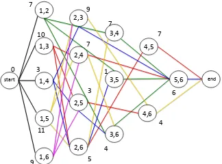
node and an endnode are added as the first (level 0) and the last level of the graph, respectively. The weights of the start and the end nodes are both 0. The edges between the nodes are dynamically established as the algorithm of finding the optimal solution progresses. Such organization of the graph nodes will be used to help reduce the time complexity of the co-scheduling algorithms proposed in this paper. Figure 1 illustrates the case where 6 jobs are co-scheduled to 2-core processors. The figure also shows how to code the node IDs in the graph and how to organize the nodes into different levels. Note that for the clarity we did not draw all edges.
1,2
1,3
1,4
1,5
1,6 2,3
2,4
2,5
2,6 3,4
3,5
3,6 4,5
4,6 5,6
start end
0 7
10
3
11
9
9
7
3
5 4 1 7
7
[image:5.612.93.255.523.643.2]4 6
Fig. 1: The exemplar co-scheduling graph for co-scheduling 6 jobs on Dual-core machines; the list of numbers in each node is the node ID; A number in a node ID is a job ID; The edges of the same color form the possible co-scheduling solutions; The number next to the node is the node weight, i.e., total degradation of the jobs in the node.
In the constructed co-scheduling graph, a path from the start to the end node forms a co-scheduling solution if the path does not contain duplicated jobs, which is called a valid path. The distance of a path is defined as the sum of the weights of all nodes on the path. Finding the optimal co-scheduling solution is equivalent to finding the shortest valid path from the start to the end node. It is straightforward to know that a valid path contains at most one node from each level in the graph.
2) The intuitive strategies to solve the graph model:
Intuitively, we first tried to solve the graph model using Dijkstra’s shortest path algorithm [9]. However, we found that Dijkstra’s algorithm can not be directly applied to find the correct solution. This can be illustrated using the example in Figure 1. In order to quickly reveal the problem, let us consider only five nodes in Figure 1, h1,5i,h1,6i,h2,3i,h4,5i,h4,6i. Assume the weights of these nodes are 11, 9, 9, 7 and 4, re-spectively. Out of all these five nodes, there are two valid paths reaching nodeh2,3i:hh1,5i,h2,3iiandhh1,6i,h2,3ii. Since the distance ofhh1,6i,h2,3ii, which is 18, is shorter than that of hh1,5i,h2,3ii, which is 20, the path hh1,6i,h2,3ii will not been examined again according to Dijkstra’s algorithm. In order to form a valid schedule, the path hh1,6i,h2,3ii has to connect to node h4,5i to form a final valid path hh1,6i,h2,3i,h4,5ii with the distance of 25. However, we can see thathh1,5i,h2,3i,h4,6iiis also a valid schedule and its distance is less than that of hh1,6i,h2,3i,h4,5ii. But the schedule of hh1,5i,h2,3i,h4,6ii is dismissed by Dijkstra’s algorithm during the search for the shortest path.
The main reason for this is because Dijkstra’s algorithm only records the shortest subpaths reaching up to a certain node and dismisses other optional subpaths. This is fine for searching for the shortest path. But in our problem, we have to search for the shortest VALID path. After Dijkstra’s algorithm searches up to a certain node in the graph and only records the shortest subpath up to that node, not all nodes among the unsearched nodes can form a valid schedule with the current shortest subpath, which may cause the shortest subpath to connect to the nodes with bigger weights. On the other hand, some subpath that has been dismissed by Dijkstra’s algorithm may be able to connect to the unsearched nodes with smaller weights and therefore generates a shorter final valid path.
IV. SHORTEST VALID PATH FOR SERIAL JOBS
A. The SVP algorithm
In order to tackle the problem that Dijkstra’s algorithm may not find the shortest valid path, the following dismiss strategy is adopted by the SVP algorithm:
SVP records all jobs that an examined sub-path contains. Assume a set of sub-paths,S, each of which contains the same set of jobs (the set of graph nodes that these paths traverse are different). SVP only keeps the path with the smallest distance and other paths are dismissed and will not be considered any more in further searching for the shortest path.
It is straightforward to know that the strategy can improve the efficiency comparing with the intuitive, enumerative strat-egy, i.e., the SVP algorithm examines much less number of subpaths than the enumerative strategy. This is because for all different subpaths that contain the same set of jobs, only one subpath (the shortest one) will spawn further subpaths and other subpaths will be discarded.
The SVP algorithm is outlined in Algorithm 1. The main differences between SVP and Dijkstra’s algorithm lie in three aspects. 1) The invalid paths, which contain the duplicated jobs, are disregarded by SVP during the searching. 2) The dismiss strategy is implemented. 3) No edges are generated between nodes before SVP starts and the node connections are established as SVP progresses. This way, only the node connections spawned by the recorded subpaths will be gener-ated and therefore further improve the performance.
The time complexity of Algorithm 1 is O
m
P
i=1
n−i i·(u−1)
·
((n−u+ 1) + ( n
u)
n−u+1+log
n u
), wheremis the number of
u-core machines required to runnjobs. The detailed analysis of the time complexity is presented in the supplementary file.
B. Further optimization of SVP
One of the most time-consuming steps in Algorithm 1 is to scan every node in a valid level to find a valid node for a given subpath v.path (Line 11 and 28). Theorem 1 is introduced to reduce the time spent in finding a valid node in a valid level. The rational behind Theorem 1 is that once the algorithm locates a node that contains a job appearing in v.path, the number of the nodes that follow that node and also contains that job can be calculated since the nodes are arranged in the ascending order of node ID. These nodes are all invalid and can therefore be skipped by the algorithm.
Theorem 1. Given a subpath v.path, assume that levell is
a valid level and node k (assume node k contains the jobs,
j1, ..., ji, ..., ju) is the first node that is found to contain a job
(assume the job isji) appearing inv.path. Then, jobji must
also appear in the next n−ji
u−i
nodes in the level.
Proof:Since the graph nodes in a level is arranged in the ascending order of node ID, the number of nodes whose i-th job is ji equals to the number of possibilities of mapping the
jobs whose IDs are bigger thanji to(u−i)positions, which
can be calculated by n−ji
u−i
.
Algorithm 1: The SVP Algorithm
1:SVP(Graph)
2: v.jobset={Graph.start}; v.path=Graph.start;
v.distance= 0; v.level= 0; 3: add v into Q;
4: Obtain v from Q;
5: while Graph.end is not in v.jobset
6: for every level l from v.level+ 1 to
Graph.end.level do
7: if job l is not in v.jobset
8: valid_l=l;
9: break;
10: k= 1;
11: while k≤ n−valid_l u−1
12: if nodek.jobset∩v.jobset=φ
13: distance=v.distance+nodek.weight;
14: J=v.jobset∪nodek.jobset;
15: if J is not in Q
16: Create an object u for J; 17: u.jobset=J;
18: u.distance=distance; 19: u.path=v.path+nodek;
20: u.level=nodek.level
21: Add u into Q;
22: else
23: Obtain u0 whose u0.jobset is J; 24: if distance < u0.distance
25: u0.distance=distance; 26: u0.path=v.path+nodek;
27: u0.level=node
k.level
28: k+ = 1; 29: Remove v from Q;
30: Obtain the v with smallest v.distance from Q; 31: return v.path as the shortest valid path;
Based on Theorem 1, the O-SVP (Optimal SVP) algorithm is proposed to further optimize SVP. The only difference between O-SVP and SVP is that in the O-SVP algorithm, when the algorithm gets to an invalid node, instead of moving to the next node, it calculates the number of nodes that can be skipped and jumps to a valid node. Effectively, O-SVP can find a valid node in the time of O(1). Therefore, the time
com-plexity of O-SVP isO
m
P
i=1
n−i i·(u−1)
·((n−u+ 1) +log nu
)
.
The algorithm outline for O-SVP is omitted in this paper. In summary, SVP accelerates the solving process over the enumerative method by reducing the length of Q in the algo-rithm, while O-SVP further accelerates over SVP by reducing the time spent in finding a valid node in a level.
V. SHORTEST VALID PATH FOR PARALLEL JOBS
The SVP algorithm presented in last section considers only serial jobs. This section addresses the co-scheduling of both serial and Parallel jobs. Subsection 5.1 presents how to handle Embarrassingly Parallel (PE) jobs, while Subsection 5.2 further extends the work in Subsection 5.1 to handle the parallel jobs with inter-process Communications (PC) jobs.
A. Co-scheduling PE jobs
Algorithm 2: The SVPPE algorithm
1: SVPPE(Graph, start, end):
2-12: ... //same as Line 2-12 in Algorithm 1;
13: total_dg_serial=v.dg_serial+nodek.dg_serial
14: for every parallel job, pi, in nodek:
15: if pi in v.jobset:
16: dg_pi=max(v.dg_pi, nodek.dg_pi);
17: else
18: dg_pi=nodek.dg_pi;
19: distance=P
dg_pi+total_dg_serial;
20-26: ... //same as Line14-20 in Algorithm 1
27: u.dg_serial=total_dg_serial;
28: for every parallel job, pi, in nodek do
29: u.dg_pi=dg_pi;
30-36: ... //same as Line21-27 in Algorithm 1
37: u0.dg_serial=total_dg_serial;
38: for every parallel job, pi, in nodek do
39: u0.dg_pi=dg_pi;
40-43: ... //same as Line28-31 in Algorithm 1
5.1.2 presents the optimization techniques to accelerate the solving process of SVPPE.
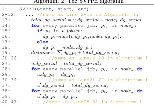
1) The SVPPE algorithm: When Algorithm 1 finds a valid node, it calculates the new distance after the current path extends to that node (Line 13). The calculation is fine for serial jobs, but cannot be applied to parallel jobs. As discussed in Subsection 3.2, the finish time of a parallel job is determined by Eq. 5. In order to incorporate parallel jobs, we can treat each process of a parallel job as a serial job (therefore the graph model remains the same) and extend the SVP algorithm simply by changing the way of calculating the path distance. In order to calculate the performance degradation for PE jobs, a few new attributes are introduced. First, two new attributes are added to an object v in Q. One attribute stores the total degradation of all serial jobs on v.path (denoted by v.dg serial). The other attribute is an array, in which each entry stores the biggest degradation of all processes of a parallel job pi onv.path (denoted by v.dg pi). Second, two
similar new attributes are also added to a graph node nodek.
One stores the total degradation of all serials jobs in nodek
(denoted by nodek.dg serial). The other is also an array, in
which each entry stores the degradation of a parallel jobpiin nodek (denoted by nodek.dg pi).
SVPPE is outlined in Algorithm 2. The only differences between SVPPE and SVP are: 1) changing the way of calcu-lating the subpath distance (Line 13-19 in Algorithm 2), and 2) updating the newly introduced attributes for the case whereJ
is not inQ(Line 28-30) and the case otherwise (Line 38-40). The maximum number of the iterations of all for-loops (Line 14, 28 and 38) is u, because there are most u jobs in a node. Each iteration takes the constant time. Therefore, the worst-case complexity of computing the degradation (the first for-loop) and updating the attributes (two other for-loops) are O u. Therefore, combining with the time complexity of Algorithm 1, the worst-case complexity of Algorithm 2 is
O
m
P
i=1
n−i i·(u−1)
·((n−u+ 1) +u· ( n
u)
n−u+1+log
n u
)
.
2) Process condensation for optimizing SVPPE: An obvi-ous optimization measure for SVPPE is to skip the invalid nodes in the similar way as that given in Theorem 1, which is not repeated in this Subsection. This subsection focuses on proposing another important optimization technique that is only applicable to PE jobs. The optimization technique is based on this observation: different processes of a parallel job should have the same mutual effect with other jobs. So it is unnecessary to differentiate different processes of a parallel job, treating them as individual serial jobs.
Therefore, the optimization technique, which is called the
process condensation techniquein this paper, labels a process of a parallel job using its job ID, that is, treats different processes of a parallel job as the same serial job. We illustrate this below using Figure 1. Now assume the jobs labelled 1, 2, 3 and 4 are four processes of a parallel job, whose ID is set to be 1. Figure 1 can be transformed to Figure 2 after deleting the same graph nodes in each level (the edges are omitted). Comparing with Figure 1, it can be seen that the number of graph nodes in Figure 2 is reduced. Therefore, the number of subpaths that need to be examined and consequently the time spent in finding the optimal solution is significantly reduced.
S S 1,5
1,1
1,6 1,5 1,1
1,6 1,5 1,1
1,6 1,5
[image:7.612.46.298.67.241.2]1,6 5,6
Fig. 2: The graph model for a mix of serial and parallel jobs
We now present the O-SVPPE (Optimal SVPPE) algorithm, which adjusts SVPPE so that it can find the shortest valid path in the optimized co-scheduling graph. The only difference between O-SVPPE and SVPPE is that a different way is used to find 1) the next valid level and 2) a valid node in a valid level for parallel jobs.
Line 6-9 in Algorithm 1 is the way used by SVPPE to find the next valid level. In O-SVPPE, for a given level l, if job
l is a serial job, the condition of determining whether level
l is valid is the same as that in SVPPE. However, since the same job ID is now used to label all processes of a parallel job, the condition of whether a job ID appears on the given subpath cannot be used any more to determine a valid level for parallel jobs. The correct method is discussed next.
Several new attributes are added for the optimized graph model.proci denotes the number of processes that parallel job pi has. For a given subpathv.path,v.proci is the number of
times a process of parallel jobpi appears onv.path.v.jobset
is now a bag (not set) of job IDs that appear on v.path, that is, there arev.proci instances of that parallel job inv.jobset.
Same as the case of serial jobs, the adjustedv.jobsetis used to determine whether two subpaths consists of the same set of jobs (and parallel processes). A new attribute,nodek.jobset,
is also added to a graph node nodek, where nodek.jobset
is also a bag of job IDs that are in nodek. nodek.proci is
Algorithm 3: The O-SVPPE algorithm
1: O-SVPPE(Graph)
2-6: ... //same as Line 2-6 in Algorithm 1;
7: if job l is a serial job
8-10: ...// same as Line 7-9 in Algorithm 1;
11: else if v.procl< procl
12: validl=l;
13: break;
14-15: ... //same as Line 10-11 in Algorithm 1
16: if nodek.serialjobset∩v.jobset=φ & ∀pi,
v.proci+nodek.proci≤proci
17-48: ... //same as Line13-44 in Algorithm 2
nodek.serialjobsetis a set of all serial jobs innodek.
Theorem 2 gives the condition of determining whether a level is a valid level for a given path.
Theorem 2. Assume job l is a parallel job. For a given subpath
v.path, level l (l starts from v.level+ 1) is a valid level if
v.procl< procl. Otherwise, level l is not a valid level.
Proof: Assume the jobs are co-scheduled on u-core machines. Let U be the bag of jobs that includes all serial jobs and parallel jobs (the number of instances of a parallel job inU equals to the number of processes that that job has). LetD=U−v.jobset.Xdenotes all possible combinations of selectingu−1jobs fromD. Because of the way that the nodes are organized in the graph, the last u−1 jobs of the nodes in levell must include all possible combinations of selecting
u−1jobs from a set of jobs whose ID are the range oflton
(nis the number of jobs to be co-scheduled), which is denoted byY. Then we must haveX∩Y 6=φ. This means that as long as the ID of the first job in the nodes in level lis not making the nodes invalid, which can be determined by the condition
v.procl< procl, we must be able to find a node in levellthat
can append to v.pathand form a new valid subpath.
After a valid level is found, O-SVPPE needs to find a valid node in that level. When there are both parallel and serial jobs, O-SVPPE uses two conditions to determine a valid node: 1) the serial jobs in the node do not appear in v.jobset, and 2) ∀ parallel jobpi in the node,v.proci+nodek.proci≤proci.
O-SVPPE is outlined in Algorithm 3, in which Line 7-13 implements the way of finding a valid level and Line 16 checks whether a node is valid, as discussed above.
B. Co-scheduling PC jobs
This subsection extends the SVPPE algorithm to handle PC jobs, which is called SVPPC (SVP for PC jobs). We first model the communication time,cij,S, in Eq. 5 and then adjust SVPPE
to handle PC jobs. Moreover, since the further optimization technique developed for PE jobs, i.e., the O-SVPPE algorithm, presented in Subsection 5.1.2 cannot be directly applied to PC jobs, the O-SVPPE algorithm is extended to handle PC jobs in Subsection 5.2.2, called O-SVPPC.
1) Modelling the communications in PC jobs: cij,S can
be modelled using Eq. 6, where γij is the number of the
neighbouring processes that process pij has corresponding to
the decomposition performed on the data set to be calculated by the parallel job,αij(k)is the amount of data thatpij needs
to communicate with itsk-th neighbouring process, B is the bandwidth for inter-processor communications (typically, the communication bandwidth between the machines in a cluster is same),bij(k)ispij’sk-th neighbouring process, andβij(k, S)
is 0 or 1 as defined in Eq. 6b. βij(k, S) is 0 if bij(k) is in
the job set S co-running with pij. Otherwise, βij(k, S)is 1.
Essentially, Eq. 6 calculates the total amount of data that pij
needs to communicate, which is then divided by the bandwidth
B to obtain the communication time. Note thatpij’s
commu-nication time can be determined by only examining which neighbouring processes are not in the job set S co-running with pij, no matter which machines that these neighbouring
processes are scheduled to. In the supplementary file of this paper, an example is given to illustrate the calculation ofcij,S.
cij,S=
1
B γij X
k=1
(αij(k)·βij(k, S)) (6a)
βij(k, S) =
0 ifbij(k)∈S
1 ifbij(k)∈/S
(6b)
We now adjust SVPPE to incorporate the PC jobs. In the graph model for serial and PE jobs, the weight of a graph node is calculate by summing up the weights of the individual jobs/processes, which is the performance degradation. When there are PC jobs, a process belongs to a PC job, the weight of a process pij in a PC job should be calculated by Eq. 5
instead of Eq. 1. The rest of the SVPPC algorithm is exactly the same as SVPPE.
2) Communication-aware process condensation for opti-mizing SVPPC: The reason why the process condensation technique developed for PE jobs cannot be directly applied to PC jobs is because different processes in a PC job may have different communication patterns and therefore cannot be treated as identical processes. After carefully examining the characteristics of the typical inter-process communication patterns, a communication-aware process condensation tech-nique is developed to accelerate the solving process of SVPPC, which is called O-SVPPC (Optimized SVPPC) in this paper.
VI. CO-SCHEDULING JOBS ON MULTI-PROCESSOR COMPUTERS
In order to add more cores in a multicore computer, there are two general approaches: 1) increasing the number of cores on a processor chip and 2) installing in a computer more processors with the number of cores in each processor remaining unchanged. The first approach becomes increasingly difficult as the number of cores on a processor chip increases. For example, as shown in the latest Top500 supercomputer list published in November 2014 [6], there are only 8 “cores per socket” in 46.4% supercomputers (i.e., 232). In order to produce a multicore computer with even more cores (e.g., more than 12 cores), the second approach is often adopted.
The co-scheduling graph presented in previous sections is for multicore machines each of which contains a single multi-core processor, which we now call single processor multimulti-core machines (single processor for short). If there are multiple core processors in a machine, which is called a multi-processor machine, the resource contention, such as cache contention, is different. For example, only the cores on the same processor share the Last-Level Cache (LLC) on the chip, while the cores on different processors do not compete for cache. In a single processor machine, the job-to-core mapping does not affect the tasks’ performance degradation. But it is not the case in a multi-processor machine, which is illustrated in the following example.
Consider a machine with two dual-core processors (proces-sors p1 and p2) and a co-run group with 4 jobs (j1, ..., j4).
Now consider two job-to-core mappings. In the first mapping, jobsj1 andj2are scheduled on processorp1 whilej3 andj4
on p2. In the second mapping, jobsj1 andj3 are scheduled
on processor p1 while j2 and j4 on p2. The two mappings
may generate different total performance degradations for this co-run group. In the co-scheduling graph in previous sections, a graph node corresponds to a possible co-run group in a machine, which is associated with a single performance degradation value. This holds for single processor machine. As shown in the above discussions, however, a co-run group may generate different performance degradations in a multi-processor machine, depending on the job-to-core mapping within the machine. This subsection presents how to adjust the methods presented in previous sections to find the optimal co-scheduling solution in multi-processor machines.
A straightforward method is to generate multiple nodes in the co-scheduling graph for a possible co-run group, with each node having a different weight that equals to a different performance degradation value (which is determined by the specific job-to-core mappings). We all this method MNG (Multi-Node for a co-run Group) method. For a machine withp
processors and each processor havingucores, it can be
calcu-lated that there are
p−1
Q
i=0(
(p−i)·u
u )
p! different job-to-core mappings
that may produce different performance degradations. Then the algorithms presented in previous sections can be used to find the shortest path in this co-scheduling graph and the shortest
path must correspond to the optimal co-scheduling solution on the multi-processor machines. In this straightforward solu-tion, however, the scale of the co-scheduling graph (i.e., the
number of graph nodes) increases by
p−1
Q
i=0(
(p−i)·u
u )
p! folds, and
consequently the solving time increases significantly compared with that for the case of single processor machines.
We now propose a method, called the Least Performance Degradation (LPD) method, to construct the co-scheduling graph. Using this method, the optimal co-scheduling solu-tion for multi-processor machines can be computed without increasing the scale of the co-scheduling graph. The LPD method is explained below.
As discussed above, in the case of multi-processor ma-chines, a co-run group may produce different performance degradation in a multi-processor machine. Instead of gener-ating multiple nodes (each being associated with a different weight, i.e., a different performance degradation value) in the co-scheduling graph for a co-run group, The LPD method con-structs the co-scheduling graph for multi-processor machines in the following way:A node is generated for a co-run group and the weight of the node is set to be the least performance degradation among all possible performance degradations generated by the co-run group. The rest of the construction process is exactly the same as that for the case of single processor machines.
Theorem 3 proves that from the co-scheduling graph con-structed by the LPD method, the algorithms proposed in previous sections for the case of single processor machines can still obtain the optimal co-scheduling solution on multi-processor machines.
Theorem 3. Assume the jobs are to be co-scheduled on
multi-processor machines. Using the LPD method defined above to construct the co-scheduling graph, the algorithms that have been proposed to find the optimal co-scheduling solutions on single processor machines can still find the optimal co-scheduling solutions on the multi-processor machines.
VII. CO-SCHEDULING MULTI-THREAD JOBS
A parallel job considered so far in this paper is one consisting of multiple processes, such as an MPI job. In this subsection, we adapt the proposed graph model and algorithms so that it can handle parallel jobs consisting of multiple threads, such as OpenMP jobs. We now call the former parallel jobs as Process Parallel (MPP) jobs and the latter Multi-Thread Parallel (MTP) jobs.
In the co-scheduling graph, a thread in an MTP job is treated in the same way as a parallel process in an MPP job. Comparing with MPP jobs, however, MTP jobs have the following different characteristics: 1) multiple threads of a MTP job must reside in the same machine, and 2) the communication time between threads can be neglected. According to these features, the co-scheduling graph model is adjusted as follows to handle the MTP jobs. For each node (i.e., every possible co-run group) in the co-scheduling graph, we check whether all threads belonging to the MTP are in the node. If not, the node is deleted from the graph since it does not satisfy the condition that all threads of a MTP job must reside in the same machine. We call the above process the validity check for MTP jobs.
Since the communication time between the threads in MTP jobs can be neglected, the performance degradation of a MTP job can be calculated using Eq. 3 that is used to compute the performance degradation of a PE job. Also, since the communication of a MTP job is not considered, an intuitive method to find the optimal co-scheduling solution in the existence of MTP jobs is to use the algorithm for handling PE jobs, i.e., Algorithm 3. However, after a closer look into the features of MTP jobs, we realize that Algorithm 3 can be adjusted to improve the performance for handling MTP jobs, which is explained next.
First, after the validity check for MTP jobs, all threads belonging to a MTP job must only appear in the same graph node. Therefore, there is no need to perform the process con-densation as we do in the existence of PE jobs. Consequently, the SVPPE algorithm (i.e., Algorithm 2) can be used to handle the MTP jobs. Second, when the current path expands to a new node in the SVPPE Algorithm, for each parallel job pi in the
new node SVPPE needs to check whether pi appears in the
current path. However, all threads in a MTP job only reside in the same node. Therefore, if a new node that the current path tries to expand to contain a MTP job, it is unnecessary to check whether some threads of the MTP job appear in the current path.
In order to differentiate it from SVPPE, the algorithm for finding the optimal co-scheduling solution for the mix of serial and MTP jobs is denoted as SVPPT (T stands for thread). The only difference between SVPPT and SVPPE is that Lines 15-17 in SVPPE (i.e., Algorithm 2) are removed from SVPPT.
From the above discussions, we can know that it would be much more efficient to find the optimal co-scheduling solution for MTP jobs than for PE jobs. This is because 1) the number of nodes in the co-scheduling graph for SVPPT is much less
than that for PE jobs because of the validity check for MTP jobs and 2) SVPPT does not run Lines 15-17 in SVPPE.
Note that the method discussed above for handling MTP jobs is applicable to both single processor machines and multi-processor machines.
VIII. THEA*-SEARCH-BASED ALGORITHM
The dismiss strategy designed for the SVP algorithm in Subsection 4.1 and the optimization strategies developed in O-SVPPE and O-SVPPC can avoid unnecessary searches in the co-scheduling graph. It has been shown that the A*-search algorithm is also able to find the optimal solution and during the searching, effectively prune the graph branches that will not lead to the optimal solution. In order to further accelerate the solving process, an A*-search-based algorithm is devel-oped in this section to combine the ability of avoiding the unnecessary searches in the traditional A*-search algorithm and the algorithms presented in this paper so far (SVP, O-SVP, O-SVPPE and O-SVPPC).
This section presents how to design the A*-search-based algorithm to find the optimal co-scheduling solution in the scheduling graph. In this section, we only consider the co-scheduling of serial and PC jobs for the sake of generality. The presented A*-search-based algorithm is called SVPPC-A*. SVP-A* (i.e., co-scheduling serial jobs), SVPPE-A* (i.e., co-scheduling both serial and PE jobs) and SVPPT-A* can be developed in similar ways.
The traditional A*-search algorithm, which is briefly overviewed in the supplementary file, cannot be directly applied to find the optimal co-scheduling solution in the constructed co-scheduling graph due to the same reasons discussed when we present the SVP and the SVPPE algo-rithm, namely, i) the optimal co-scheduling solution in the constructed co-scheduling graph corresponds to the shortest VALID path, not the shortest path, and ii) since the jobs to be scheduled contain parallel jobs, the distance of a path is not the total weights of the nodes on the path, as calculated by the traditional A*-search algorithm.
Three functions are defined in the traditional A*-search algorithm. Function g(v)is the actual distance from the start node to nodevandh(v)is the estimated length fromvto the end node, whilef(v)is the sum ofg(v)andh(v). In SVPPC-A*, we use the exactly same methods proposed for the SVP algorithm (i.e., the dismiss strategy) to handle and expand the valid subpaths and avoid the unnecessary searches. Also, we use the method proposed for the SVPPC algorithm to calculate the distance of the subpaths (i.e., Eq. 3 and Eq. 5) that contain the PC jobs. This can used to obtain the value ofg(v). Note that the communication-aware process condensation technique proposed in Subsection 5.2.2 can also be used to accelerate SVPPC-A*.
closer the result ofh(v)is from the real lowest cost, the more effective A* search is in pruning the search space.
Therefore, in order to find the optimal solution, the h(v) function must satisfy the first property. In our problem, if there are qjobs on the path corresponding tog(v), then the aim of setting theh(v)function is to find a function of the remaining
n−q jobs such as the value of the function is less than the shortest distance from nodev to the end node. The following two strategies are proposed to set the h(v)function.
Strategy 1 for setting h(v): Assume node v is in level l, we construct a set R that contains all the nodes froml+ 1
to the last level in the co-scheduling graph, and sort these nodes in ascending order of their weights. Then, regardless of the validity, the first(n−q)/u(uis the number of cores) nodes are selected fromRto form a new subpath, and use its distance as h(v).
Strategy 2 for settingh(v): Assume nodevis in levell. We find all valid levels from levell+ 1to the last level in the co-scheduling graph. The total number of valid levels obtained must be (n−q)/u. We then obtain the node with the least weight from each valid level.(n−q)/unodes will be obtained. We use these(n−q)/unodes to form a new subpath and use its distance ash(v).
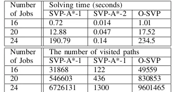
It is easy to prove thath(v)set in the above strategies must be less than the actual shortest distance from v to the end node, because it uses the nodes with the smallest weights from all remaining nodes in Strategy 1 or from all valid levels in Strategy 2. We will show in the experiments that Strategy 2 is much more effective than Strategy 1 in terms of pruning unnecessary searches.
IX. CLUSTERING APPROXIMATION FOR FINDING THE SHORTEST VALID PATH
In the previous sections, the methods and optimization strategies are presented to solve the graph model for the shortest valid path. In order to further shorten the solving time and strike the balance between solving efficiency and solution quality, this section proposes a flexible technique, called the
clustering technique, to find the approximate solution. The clustering technique is flexible because the solving efficiency can be adjusted by setting the desired solution quality. It can be applied to both O-SVP, O-SVPPE and O-SVPPC.
As discussed in introduction and related work, the reason why co-scheduling causes performance degradation is because the co-run jobs compete for the shared cache. SDC (Stack Distance Competition) is a popular technique to calculate the impact when multiple jobs are co-running, which takes the SDPs (Stack Distance Profile) of the multiple jobs as input. Therefore, if two jobs have similar SDPs, they will have similar mutual effect with other co-running jobs. The fundamental idea of the proposed clustering technique is to class the jobs with similar SDPs together and treat them as the same job. Reflected in the graph model, the jobs in the same class can be given the same job ID. In doing so, the number of different nodes in the graph model will be significantly reduced. The resulting effect is the same as the case where
different parallel processes are given the same job ID when we present O-SVPPE in Subsection 5.1.2.
Now we introduce the method of measuring the similarity level of SDP between two jobs. Given a job ji, its SDP
is essentially an array, in which the k-th element records the number of cache hits on the k-th cache line (which is denoted byhi[k]). The following formula is used to calculate
the Similarity Level (SL) in terms of SDP when comparing another jobjj against ji.
SL=
q
Pcl
k=1(hi[k]−hj[k])2
Pcl
k=1hi[k]
(7)
When SL is set bigger, more jobs will be classed together. Consequently, there will be less nodes in the graph model and hence less scheduling time is needed at the expenses of less accurate solution.
The clustering O-SVP algorithm is the same as the O-SVP algorithm, except that the way of finding a valid level as well as finding a valid node in a valid level is the same as that for O-SVPPE (Algorithm 3). The clustering technique can also be applied to O-SVPPE and O-SVPPC in a similar way. The detailed discussions are not repeated.
X. EVALUATION
This section evaluates the effectiveness and the efficiency of the proposed methods: O-SVP, O-SVPPE, O-SVPPC, A*-search-based algorithms (i.e., SVPPC-A* and SVP-A*) and the Clustering approximation technique. In order to evaluate the effectiveness, we compare the algorithms proposed in this paper with the existing co-scheduling algorithms proposed in [16]: Integer Programming (IP), Hierarchical Perfect Matching (HPM), Greedy (GR).
A further 8MB 16-way L3 cache is shared by the four cores. The 8 core machine has two Intel Xeon L5520 processors with each processor having 4 cores. Each core has a dedicated 32KB L1 cache and a dedicated 256KB L2 cache, and 8MB 16-way L3 cache shared by 4 cores. The 16 core machine has two Intel Xeon E5-2450L processors with each processor having 8 cores. Each core has a dedicated 32KB L1 cache and a dedicated 256KB L2 cache, and 16-way 20MB L3 cache shared by 8 cores. The network interconnecting the dual-core and quad-core machines is the 10 Gigabit Ethernet, while the network interconnecting 8-core and 16-core Xeon machines is QLogic TrueScale 4X QDR InfiniBand. In the rest of this section, we label 8 core and 16 core machines as 2*4 core and 2*8 core machines to show that they are dual-processor machines.
The single-run computation times of the benchmarking programs are measured. Then the method presented in [23] is used to estimate the co-run computation times of the programs, the details of which are presented in the supplementary file. With the single-run and co-run computation times, Eq. 1 is then used to compute the performance degradation.
In order to obtain the communication time of a parallel process when it is scheduled to co-run with a set of job-s/processes, i.e.,cij,S in Eq. 6, we examined the source codes
of the benchmarking MPI programs used for the experiments and obtained the amount of data that the process needs to communicate with each of its neighbouring processes (i.e.,
αij(k)in Eq. 6). Then Eq. 6 is used to calculatecij,S.
A. Evaluating the O-SVP algorithm
In this subsection, we compare the O-SVP algorithm with the existing co-scheduling algorithms in [16].
These experiments use all 10 serial benchmark programs from the NPB-SER suite. The results are presented in 3a and 3b, which show the performance degradation of each of the 10 programs plus their average degradation under different co-scheduling strategies on Dual-core and Quad-core machines.
The work in [16] shows that IP generates the optimal co-scheduling solutions for serial jobs. As can be seen from Figure 3a, O-SVP achieves the same average degradation as that under IP. This suggests that O-SVP can find the optimal co-scheduling solution for serial jobs. The average degradation produced by GR is 15.2%worse than that of the optimal solution. It can also been seen from Figure 3a that the degradation of FT is the biggest among all 10 benchmark programs. This may be because FT is the most memory-intensive program among all, and therefore endures the biggest degradation when it has to share the cache with others.
Figure 3b shows the results on Quad-core machines. In this experiment, in addition to the 10 programs from NPB-SER, 6 serial programs (applu, art, ammp, equake, galgel and vpr) are selected from SPEC CPU 2000. In Figure 3b, O-SVP produces the same solution as IP, which shows the optimality of O-SVP. Also, O-SVP finds the better co-scheduling solution than HPM and GR. The degradation under HPM is7.7%worse than that under O-SVP, while that of GR is 25.5% worse. It is worth
noting that O-SVP does not produce the least degradation for all programs. The aim of O-SVP is to produce minimal total degradation. This is why O-SVP produced bigger degradation than GR and HPM in some cases.
B. The O-SVPPE algorithm
The reasons why we propose O-SVPPE are because 1) none of the existing co-scheduling methods is designed for parallel jobs; 2) we argue that if applying the existing co-scheduling methods designed for serial jobs to schedule parallel jobs, it will not produce the optimal solution. In order to investigate the performance discrepancy between the method for serial jobs and that for PE jobs, we apply O-SVP to solve the co-scheduling for a mix of serial and parallel jobs and compare the results with those obtained by O-SVPPE. In the mix of serial and parallel jobs, the parallel jobs are those 5 embarrassively parallel programs (each with 12 processes) and the serial jobs are from NPB-SER plus art from SPEC CPU 2000. The experimental results are shown in Figure 4a and 4b As can be seen from the figures, SVPPE produces smaller average degradation than O-SVP in both Dual-core and Quad-core cases. In the Dual-Quad-core case, the degradation under O-SVP is worse than that under O-SVPPE by 9.4%, while in the Quad-core case, O-SVP is worse by 35.6%. These results suggest it is necessary to design the co-scheduling method for parallel jobs.
C. The O-SVPPC algorithm
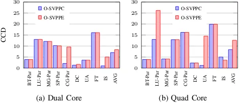
Figure 5a and 5b show the Communication-Combined Degradation (CCD) (i.e., the value of Eq. 5) of the co-scheduling solution obtained by the SVPPC algorithm when the applications are run on Dual-core and Quad-core, respec-tively. In this set of experiments, 5 MPI applications (i.e., BT-Par, LU-BT-Par, MG-BT-Par, SP-Par and CG-Par) are selected from the NPB3.3-MPI suite and each parallel application is run using 10 processes, while the serial jobs remain the same as those used in Fig. 4b. In order to demonstrate the effectiveness of the SVPPC, SVPPE is also used find the co-scheduling solution for the mix of MPI jobs and serial jobs, by ignoring the inter-process communications in the MPI jobs. We then use Eq. 5 to calculate CCD of the co-scheduling solution obtained by SVPPE. The resulting CCD is also plotted in Figure 5a and 5b. As can be seen from these figures, the CCD under SVPPE is worse than that under SVPPC by 18.7% in Dual-core machines, while in Quad-core machines, the CCD obtained by SVPPE is worse than that by SVPPC by 50.4%. These results justifies the need to specially develop the algorithm to find the co-scheduling solution for PC jobs.
BT CG FT DC EP IS LU MG SP UA AVG
0 1 2 3 4 5 6 7 8
De
gradation
O-SVP IP GR
(a) Dual Core
BT CG FT DC EP IS LU MG SP UA applu art ammp equake galgel vpr AVG
0 1 2 3 4 5 6 7 8
O-SVP IP HPM GR
[image:13.612.57.567.65.144.2](b) Quad Core
Fig. 3: Comparing the degradation of serial jobs under O-SVP, IP, HPM and GR
PI
MMS EP RA MCM DC U
A
BT IS AVG
0 2 4 6 8 10
De
gradation
O-SVPPE
O-SVP
(a) Dual Core
PI
MMS EP RA MCM DC U
A
BT IS AVG
0 2 4 6 8
10 O-SVPPE O-SVP
[image:13.612.55.291.192.289.2](b) Quad Core
Fig. 4: Comparing the degradation under SVPPE and O-SVP for a mix of PE and serial benchmark programs
BT
-P
ar
LU-P
ar
MG-P
ar
SP-P
ar
CG-P
ar
DC UA FT IS AVG
0 5 10 15 20 25 30
CCD
O-SVPPC
O-SVPPE
(a) Dual Core
BT
-P
ar
LU-P
ar
MG-P
ar
SP-P
ar
CG-P
ar
DC UA FT IS AVG
0 5 10 15 20 25 30
O-SVPPC
O-SVPPE
(b) Quad Core
Fig. 5: Comparing the Communication-Combined Degradation (CCD) obtained by SVPPC and SVPPE
For example, 8+4*12 represents a job mix with 8 serial and 4 parallel jobs, each with 12 processes.
8 + 4∗12 4 + 4∗14 0 + 4∗16 14
16 18
CCD
O-SVPPC
O-SVPPE
(a) Increasing the number of processes
16 + 1∗4 12 + 2∗4 8 + 3∗4 4 + 4∗4 20
30 40
O-SVPPC
O-SVPPE
[image:13.612.55.291.347.448.2](b) Increasing the number of jobs
Fig. 6: Impact of the number of parallel jobs and parallel processes
In Figure 6a, the difference in CCD between SVPPC and SVPPE becomes bigger as the number of parallel processes increases. This result suggests that SVPPE performs
increas-ingly worse than SVPPC (increasing from 11.8% to 21.5%) as the proportion of PC jobs increases in the job mix. Another observation from this figure is that the CCD decreases as the proportion of parallel jobs increases. This is simply because the degradation experienced by multiple processes of a parallel job is only counted once. If those processes are the serial jobs, their degradations will be summed and is therefore bigger. In Figure 6b, the number of processes per parallel job remains unchanged and the number of parallel jobs increases. For example, 12+2*4 represents a job mix with 12 serial jobs and 2 parallel jobs, each with 4 processes. The detailed combinations of serial and parallel jobs are: i) In the case of 16+1*4, MG-Par is used as the parallel job and all 16 serial programs are used as the serial jobs; ii) In the case of 12+2*4, LU-Par and MG-Par are the parallel jobs and the serial jobs are SP, BT, FT, CG, IS, UA, applu, art, ammp, equake, galgel and vpr; iii) In the case of 8+3*4, BT-Par, LU-Par, MG-Par are parallel jobs and the serial jobs are SP, BT, FT, DC, IS, UA, equake, galgel; iv) In the case of 4+4*4, BT-Par, LU-Par, SP-Par, MG-Par are parallel jobs and the serial jobs are IS, UA, equake, galgel. The results in Figure 6b show the similar pattern as those in Figure 6a. The reasons for these results are also the same.
D. Scheduling in Multi-processor Computers
In this section, we investigate the effectiveness of the LPD method proposed to handle the co-scheduling in multi-processor machines. In the experiments, we first use the MNG method discussed in Section 6 (i.e., generating multiple graph nodes for a co-run group with each node having a different weight) to construct the co-scheduling graph. As we have discussed, from the co-scheduling graph constructed by the MNG method, the algorithm must be able to find the optimal co-scheduling solution for multi-processor machines. Then we use the LPD method to construct the graph and find the shortest path of the graph. The experimental results are presented in Figure 7a and 7b, in which a mix of 4 PE jobs (PI, MMS, RA and MCM, each with 31 processes) and 4 serial jobs (DC, UA, BT and IS) are used. It can be seen that the performance degradations obtained by two methods are the same. This result verifies that the algorithms can produce the optimal co-scheduling solutions using the LPD method.
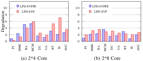
[image:13.612.53.299.552.641.2]generate the co-scheduling graphs (therefore, the ”LPD” prefix is added to the algorithms in the legends in the figures). In these experiments, we use the same experimental settings as in Figure 7a and 7b. The results are shown in Figure 8a and 8b. As can be seen from the figures, LPD-SVPPE produces smaller average degradation than LPD-SVP in both 8-core and 16-core cases. In the 8-core case, the degradation under LPD-SVP is worse than that under LPD-LPD-SVPPE by31.9%, while in the 16-core case, LPD-SVP is worse by 34.8%. These results verify the effectiveness of the LPD method for co-scheduling PE jobs.
Similarly, following the same logic as in Figure 5, we conducted the experiments to run PC jobs using SVPPC and SVPPE on multi-processor machines and compare the performance discrepancy in terms of CCD. The same exper-imental settings as in Figure 5 are used and the results are presented in Figure 9a and 9b. In this set of experiments, 4 MPI applications (i.e., BT-Par, LU-Par, MG-Par, and CG-Par) are selected from the NPB3.3-MPI suite and each parallel application is run using 31 processes, while the same serial jobs as in Fig. 7a are used. As can be seen from these figures, the CCD under LPD-SVPPE is worse than that under LPD-SVPPC by 36.1% and39.5%in 2*4-core and 2*8-core machines, respectively. These results justify the necessity of using SVPPC to handle PC jobs and show that the LPD method works well with the SVPPC algorithm.
As discussed in Section 6, the reason why we propose the LPD method is because using the MNG method, the scale of the co-scheduling graph increased significantly in multi-processor systems. The LPD method can reduce the scale of the co-scheduling graph and consequently reduce the solving time. Therefore, we also conducted the experiments to compare the solving time obtained by LPD and the MNG method. The experimental results are presented in Figure 10, in which Figure 10a and 10b are for PE and PC jobs, respectively. It can be seen from the figure that the solving time of LPD is significantly less than that of the straightforward method and the discrepancy increases dramatically as the number of jobs increases. These results suggest that LPD is effective in reducing solving time compared with the MNG method.
PI
MMS RA MCM DC U A BT IS
A
V
G
0 2 4 6 8 10
De
gradation
MNG
LPD
(a) 2*4 Core
PI
MMS RA MCM DC U A BT IS
A
V
G
0 2 4 6 8
10 MNG LPD
(b) 2*8 Core
Fig. 7: Comparing the degradation caused by the straightfor-ward method and the LPD method
PI
MMS RA MCM DC U
A
BT IS AVG
0 2 4 6 8 10
De
gradation
LPD-SVPPE
LPD-SVP
(a) 2*4 Core
PI
MMS RA MCM DC U
A
BT IS AVG
0 2 4 6 8
10 LPD-SVPPE
LPD-SVP
[image:14.612.325.554.66.165.2](b) 2*8 Core
Fig. 8: Comparing the degradation under SVP and LPD-SVPPE for a mix of PE and serial benchmark programs
BT
-P
ar
LU-P
ar
MG-P
ar
CG-P
ar
DC UA FT IS AVG
0 5 10 15 20
CCD
LPD-SVPPC
LPD-SVPPE
(a) 2*4 Core
BT
-P
ar
LU-P
ar
MG-P
ar
CG-P
ar
DC UA FT IS AVG
0 5 10 15 20
LPD-SVPPC
LPD-SVPPE
[image:14.612.319.559.229.331.2](b) 2*8 Core
Fig. 9: Comparing the Communication-Combined Degradation (CCD) obtained by LPD-SVPPC and LPD-SVPPE
E. Scheduling Multi-threading Jobs
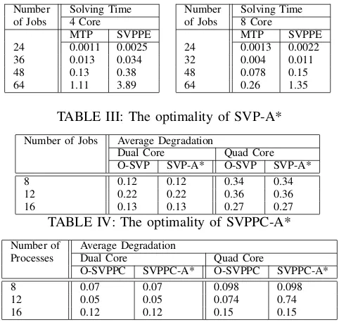
In Section 7, in order to schedule the MTP jobs correctly, we need to guarantee that the threads from the same MTP job are scheduled in the same machine. In order to handle this, the SVPPT algorithm is proposed to construct the co-scheduling graph and find the shortest path. In this subsection, we first conduct the experiments to examine the co-scheduling solution obtained by SVPPT. In the experiments, we chose 4 MTP programs (each with 2 threads on 4 Core and 3 threads on 8 Core) from NPB3.3-OMP (BT, MG, EP and FT) and 4 serial jobs from NPB-SER (DC, UA, LU and SP). The experiments are conducted on two type of processors, Xeon L5520 (4 cores) and Xeon E5-2450L (8 cores). The results are presented in Table 1. It can be seen that all threads from the same MTP program are mapped to the same machine, which verifies SVPPT can find correct co-scheduling solutions for MTP jobs.
[image:14.612.61.290.577.673.2]