Markov functional and stochastic volatility modelling

(1)

University of Warwick institutional repository: http://go.warwick.ac.uk/wrap

A Thesis Submitted for the Degree of PhD at the University of Warwick

http://go.warwick.ac.uk/wrap/55161

This thesis is made available online and is protected by original copyright.

Please scroll down to view the document itself.

(2)

AUTHOR:Duy Pham DEGREE: Ph.D.

TITLE:Markov-functional and Stochastic Volatility modelling

DATE OF DEPOSIT: . . . .

I agree that this thesis shall be available in accordance with the regulations governing the University of Warwick theses.

I agree that the summary of this thesis may be submitted for publication. I agree that the thesis may be photocopied (single copies for study purposes only).

Theses with no restriction on photocopying will also be made available to the British Library for microfilming. The British Library may supply copies to individuals or libraries. subject to a statement from them that the copy is supplied for non-publishing purposes. All copies supplied by the British Library will carry the following statement:

“Attention is drawn to the fact that the copyright of this thesis rests with its author. This copy of the thesis has been supplied on the condition that anyone who consults it is understood to recognise that its copyright rests with its author and that no quotation from the thesis and no information derived from it may be published without the author’s written consent.”

AUTHOR’S SIGNATURE: . . . .

USER’S DECLARATION

1. I undertake not to quote or make use of any information from this thesis without making acknowledgement to the author.

2. I further undertake to allow no-one else to use this thesis while it is in my care.

DATE SIGNATURE ADDRESS

. . . .

. . . . . . . .

. . . .

(3)

Markov-functional and Stochastic

Volatility modelling

by

Duy Pham

Thesis

Submitted to the University of Warwick

for the degree of

Doctor of Philosophy

Department of Statistics

(4)

List of Tables

3.1 Market data from the swaption matrix to be incorporated into the driving process x for a 11 years annual Bermudan swaption. HW’s

approach (left), alternative approach (right). . . 31

3.2 Black implied volatilities (%) of the ATM swaptions on October 17, 2007. . . 37

3.3 Initial swap rates (%) on October 17, 2007. . . 38

3.4 The Bermudan swaption’s scaled vegas (in 104_{) under the HW model. 39} 3.5 The Bermudan swaption’s scaled vegas (in 104) under the MR model. 39 3.6 The Bermudan swaption’s scaled vegas (in 104) under the one step covariance model. . . 42

3.7 The Bermudan swaption’s scaled vegas (in 104) under the weighted covariance model (α= 0.05). . . 42

3.8 The Bermudan swaption’s scaled vegas (in 104_{) under the weighted} covariance model (α= 0.3). . . 43

3.9 The Bermudan swaption’s scaled vegas (in 104) under the weighted covariance model (α= 5). . . 43

3.10 The Bermudan swaption’s scaled vegas (in 104) for the HW and MR models. . . 50

3.11 The co-terminal vanilla swaptions’ scaled vegas (in 104). . . 50

3.12 Vega hedging (N_isption) for the HW and MR models. . . 50

3.13 Delta hedging (N_iswap) for the HW and MR models (correspond to swaps with notional N = 1 million). . . 52

3.14 Scaled total gammas of the HW and MR portfolios. . . 54

3.15 The vanilla swaptions’ scaled vegas (in 104). . . 59

3.16 Vega hedging (N_i,jsption) for the one step covariance model. . . 60

3.17 Vega hedging (N_i,jsption) for the weighted covariance model (α= 0.05). 60 3.18 Vega hedging (N_i,jsption) for the weighted covariance model (α= 0.3). 61 3.19 Vega hedging (N_i,jsption) for the weighted covariance model (α= 5). . 61

(9)

3.21 Scaled total gammas of the one step and weighted covariance portfolios. 63 3.22 Contribution of the gamma >A(t) to the change in values of the

portfolios as all co-initial swap rates move up (or down) by 1 bp, i.e.

> = (±0.0001, . . . ,±0.0001). . . 66

3.23 The change in values of the portfolios as time advances by 1 trading day (theta). . . 67 3.24 Contribution of the gamma >A(t) to the change in values of the

portfolios of payer Bermudans with different strikes as all co-initial swap rates move up (or down) by 1 bp, i.e. >= (±0.0001, . . . ,±0.0001). 69 3.25 The change in values of the portfolios of payer Bermudan swaptions

with different strikes as time advances by 1 trading day (theta). . . . 69 3.26 The gamma-theta balance (∂V

port

t ∂t h+

1

2

>_A₍_t₎_{) of the portfolios of}

payer Bermudan swaptions with different strikes as co-initial swap rates move 3 bp after 1 trading day, i.e. h = 1 trading day and

> = (±0.0003, . . . ,±0.0003). . . 70

3.27 Effects of bumping the co-initial swap rates by 1 bp on the LIBORs (in percentage). The bold figures represent the main effects. . . 78 3.28 Effects of bumping the co-initial swap rates by 1 bp on the co-terminal

swap rates (in percentage). The bold figures represent the main effects. 79

5.1 Probability mass assigned to the absorbing barrier (CEV-SABR) and the negative rates region (DD-SABR) for the four cases considered in figures 5.7 and 5.8 (computed by direct Monte Carlo simulation). . . 100 5.2 Checklist of the most current approximations for the SABR model. . 106 5.3 Fitting errors, in percentages, against strike and maturity for β =

0, ν = 0.6, ρ=−0.1, F0 = 90, σ0 = 9 (approximation implied

volatil-ity minus MC volatilities). . . 116 5.4 Probability mass assigned to the negative rates region for the four

cases considered in figures 5.7 and 5.8. . . 123

7.1 Calibrated parameters for the Normal SABR and DD-SABR models for different expiries. . . 176 7.2 Parameters for the Normal SABR-MR and DD-SABR-MR models

(10)

List of Figures

2.1 Zero-coupon bond . . . 7

2.2 Deposit cashflows . . . 7

2.3 FRA cashflows . . . 8

2.4 Payers interest rate swap cashflows . . . 9

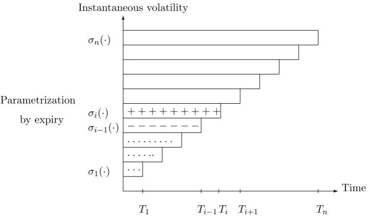
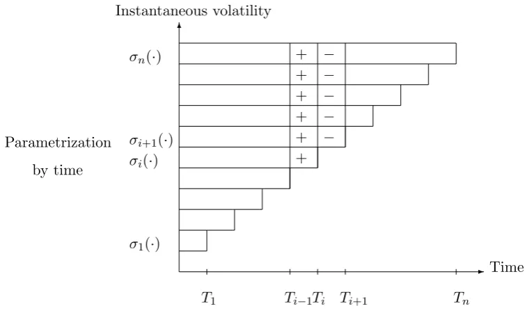
3.1 Global effect of bumping_eσi,n+1−ion the instantaneous volatility func-tions of the log-LIBORs. The dots represent a very small effect. . . . 28

3.2 Local effects of bumping the _eσi,n+1−i on the instantaneous volatility functions of the log-LIBORs. . . 30

3.3 The (net) row sum of the scaled vegas (in 104) of a 11-years annual Bermudan swaption for different models and parameters. . . 44

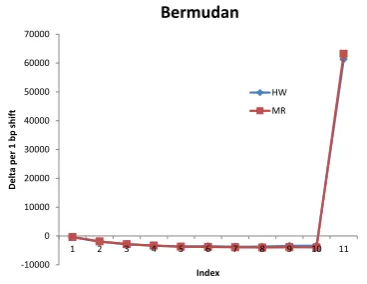
3.4 The scaled deltas of the Bermudan under the HW and MR models. . 52

3.5 Proxy vs. row sum of the gamma matrix under the HW model. . . . 53

3.6 Scaled total gamma contributions from the co-terminal vanilla swap-tions. . . 55

3.7 Scaled gamma vectors of the HW and MR portfolios before and after the hedge. . . 56

3.8 Scaled gamma contribution vectors of the co-terminal swaptions and the co-initial swaps for the HW and MR portfolios. . . 58

3.9 Scaled gamma vectors of the HW and the one step and weighted covariance portfolios before and after the hedge. . . 64

3.10 Scaled gamma contribution vectors of the vanilla swaptions and the co-initial swaps for the HW and the one step and weighted covariance portfolios. . . 65

(11)

5.2 Effects of maturityT and Volvolνon the mapping when the ATM are matched. Parameters: β = 0.5, ρ=−0.2, σ0 = 130%, F0 = 90.

MC-CEV: CEV-SABR MC solution, MC-DD: DD-SABR MC solution, Errors: MC-DD minus MC-CEV. . . 94 5.3 Effects of maturityT and Volvolνon the mapping when the ATM are

matched. Parameters: β = 0.5, ρ=−0.2, σ0 = 130%, F0 = 90.

MC-CEV: CEV-SABR MC solution, MC-DD: DD-SABR MC solution, Errors: MC-DD minus MC-CEV. . . 95 5.4 Effect of very long maturity T on the mapping when the ATM are

matched. Parameters: β= 0.5, ρ=−0.2, σ0 = 130%, F0 = 90. . . 96

5.5 Effect ofρon the mapping when the ATM are matched. Parameters:

β= 0.5, T = 10, ν = 0.3, σ0= 130%, F0= 90. . . 97

5.6 Effect ofβ on the mapping when the ATM are matched. Parameters:

ρ=−0.2, T = 10, ν = 0.3, F0 = 90,σ0 is chosen for each case so that

the ATM are comparable. . . 98 5.7 Implied volatilities under different models. Parameters: β = 0.5, ρ=

−0.2, σ0 = 4.30%,3.80% as maturity increases, respectively. . . 99

5.8 Implied volatilities under different models. Parameters: β = 0.5, ρ= −0.2, σ0 = 4.10%,3.70% as maturity increases, respectively. . . 100

5.9 The integrand of (5.12) as a function of σT. Left plot: β = 1, ρ = −0.5, F0 = 90, K = 90, T = 10, ν = 0.3, σ0 = 15%, right plot: β =

1, ρ=−0.5, F0 = 90, K = 90, T = 15, ν = 0.6, σ0= 15%. . . 105

5.10 Normal Q-Q plots: standardized conditional samples ofsT|σT against the standard Normal distribution. Common parameters: β = 1, ρ= −0.5, F0 = 90, σ0 = 5%. left plot: T = 15, ν = 0.3, σT = 5%, right plot: T = 15, ν = 0.3, σT = 50%. . . 109 5.11 Effects of maturity within a high Volvol regime on the Normal and

NIG approximations. Other parameters: β = 0, ρ = −0.1, F0 =

90, ν = 0.6, σ0 = 9. The dashed curve of the same colour indicates

the errors of the corresponding approximation. . . 114 5.12 Effects of maturity within a high Volvol regime on the Normal and

NIG approximations. Other parameters: β = 0, ρ = −0.1, F0 =

90, ν = 0.6, σ0 = 9. The dashed curve of the same colour indicates

the errors of the corresponding approximation. . . 115 5.13 Effects of moderate maturity within a low Volvol regime on the

Nor-mal and NIG approxmations. Common parameters: ν = 0.3, F0 =

90, β= 1, σ0 = 15%, ρ=−0.5. The dashed curve of the same colour

(12)

5.14 Effects of moderate maturity within a low Volvol regime on the Nor-mal and NIG approxmations. Common parameters: ν = 0.3, F0 =

90, β = 0.5, σ0 = 130%, ρ = −0.2. The dashed curve of the same

colour indicates the errors of the corresponding approximation. . . . 119 5.15 Effects of very long maturity within a low Volvol regime on the NIG

approximation. Common parameters: ν = 0.3, F0 = 90, β = 1, σ0 =

15%, ρ = −0.5. The dashed curve of the same colour indicates the errors of the corresponding approximation. . . 120 5.16 Effects of very long maturity within a low Volvol regime on the NIG

approximation. Common parameters: ν = 0.3, F0 = 90, β= 0.5, σ0=

130%, ρ= −0.2. The dashed curve of the same colour indicates the errors of the corresponding approximation. . . 121 5.17 Effect of high ν2T (stress volatility regime) on the NIG

approxima-tion. Parameters: β = 0.5, ν = 0.6, F0 = 90, σ0 = 130%, ρ = −0.2.

The dashed curve of the same colour indicates the errors of the cor-responding approximation. . . 122

6.1 Prices of forward start options for various κ: β = 0, ρ = 0, y0 =

5%, T2 = 10Y, T1= 5Y, K = 1 and calibrated parameters. . . 143

6.2 Prices of forward start options for various κ: β = 0, ρ = 0, y0 =

5%, T2 = 10Y, T1= 5Y, K = 0.75 andK = 1.25. . . 144

6.3 Prices of forward start options for various κ: β = 0.5, ρ = 0, y0 =

5%, T2 = 10Y, T1= 5Y, K = 1 and calibrated parameters. . . 145

6.4 Prices of forward start options for various κ: β = 0.5, ρ = 0, y0 =

5%, T2 = 10Y, T1= 5Y, K = 0.75 andK = 1.25. . . 146

6.5 First and second moments of the forward realized variance V_T1₂ =

RT2

T1 σ 2

tdtfor the considered cases. . . 147 6.6 ν-effect on the NIG approximation: ν= 0.4 (MC solution and

approx-imation errors). Other parameters: β = 0, y0 = 0.05, κ = 0.05, c =

0.1, ρ=−0.1. . . 154 6.7 ν-effect on the NIG approximation: ν = 0.25 (MC solution and

approximation errors). Other parameters: β = 0, y0 = 0.05, κ =

0.05, c= 0.1, ρ=−0.1. . . 155 6.8 κ-effect on the NIG approximation (MC solution and approximation

errors). Other parameters: β= 0, y0 = 0.05, ν = 0.4, c= 0.1, ρ=−0.1. 156

6.9 c-effect on the NIG approximation (MC solution and approximation errors). Other parameters: β = 0, y0 = 0.05, ν = 0.4, κ= 0.05, ρ =

−0.1. . . 157 6.10 ρ-effect on the NIG approximation (MC solution and approximation

(13)

6.11 ν-effect on the NIG approximation. . . 159

6.12 ν-effect on the NIG approximation. . . 160

6.13 κ-effect on the NIG approximation. . . 161

6.14 Stress test 1 for the NIG approximation (MC solution and approxi-mation errors). . . 162

6.15 Stress test 2 for the NIG approximation (MC solution and approxi-mation errors). . . 163

7.1 Pure deltaδ1 under the Normal SABR and DD-SABR models. . . . 176

7.2 Bartlett deltaδe₂ under the Normal SABR and DD-SABR models. . 177

7.3 Practical delta under different models. . . 180

7.4 Practical delta under different models. . . 181

7.5 Practical vega under different models. . . 182

(14)

Acknowledgments

First and foremost, I am indebted to my supervisor, Dr Jo Kennedy, for her guidance and continuous support. Jo, it wouldn’t have been possible without you. Thank you for being incredibly patient with me.

I am grateful to the department of statistics for the financial support I have received and for all the excellent lectures I have learnt from. This has been an incredible experience for me.

I would like to thank Subhankar Mitra for introducing me to the world of coding while we were working together in summer 2010. Thank you for sharing with me your invaluable experience. I am also grateful to a number of anonymous referees who provided valuable comments and suggestions to earlier versions of the papers that form the basis for this thesis.

One paragraph is surely not enough for my friends but I will try my best. First of all, a special thank to all my office mates. I can’t imagine how my office life would have been without them. Hasin and Fiona, thank you for all the joy we had together. Giorgos and Javier, those Friday glasses of wine will stay in my memory for a long time. Tomek, you are a true philosopher. Helen, 12pm Friday is always in my diary. For those who were not mentioned, I want to thank you all: from Warwick and off-Warwick, Statistics and non-Statistics. You guys have taught me so many lessons: both academic and non-academic. Thank you all for being there when it matters and spending such a priceless time at Warwick with me.

(15)

Declarations

(16)

Abstract

In this thesis, we study two practical problems in applied mathematical fi-nance. The first topic discusses the issue of pricing and hedging Bermudan swaptions within a one factor Markov-functional model. We focus on the implications for hedg-ing of the choice of instantaneous volatility for the one-dimensional drivhedg-ing Markov process of the model. We find that there is a strong evidence in favour of what we term “parametrization by time” as opposed to “parametrization by expiry”. We further propose a new parametrization by time for the driving process which takes as inputs into the model the market correlations of relevant swap rates. We show that the new driving process enables a very effective vega-delta hedge with a much more stable gamma profile for the hedging portfolio compared with the existing ones.

The second part of the thesis mainly addresses the topic of pricing European options within the popular stochastic volatility SABR model and its extension with mean reversion. We investigate some efficient approximations for these models to be used in real time. We first derive a probabilistic approximation for three different versions of the SABR model: Normal, Log-Normal and a displaced diffusion version for the general constant elasticity of variance case. Specifically, we focus on captur-ing the terminal distribution of the underlycaptur-ing process (conditional on the terminal volatility) to arrive at the implied volatilities of the corresponding European options for all strikes and maturities. Our resulting method allows us to work with a variety of parameters which cover long dated options and highly stress market condition. This is a different feature from other current approaches which rely on the assump-tion of very small total volatility and usually fail for longer than 10 years maturity or large volatility of volatility.

(17)

Chapter 1

Introduction

The purpose of this thesis is to contribute further to the current literature of two distinct areas in applied mathematical finance: Markov-functional and stochastic volatility modelling. Since the two topics have little overlap, we treat them sep-arately in Part I and Part II respectively. For each part, we provide a separate background chapter (Chapters 2 and 4) so this introductory chapter only gives a brief outline and summary of the contents of the whole thesis. Readers can choose to read the background chapter of each part and then return here for a better overview of the thesis.

Part I of the thesis discusses the issue of pricing and hedging Bermudan swaptions within a one factor Markov-functional model. We focus on the implica-tions for hedging of the choice of instantaneous volatility for the one-dimensional driving Markov process of the model. The second part of the thesis mainly addresses the topic of pricing European options within the popular stochastic volatility SABR model and its extension with mean reversion. We investigate some efficient approx-imations of the models to be used in real time.

(18)

to get a grasp of interest rate and stochastic volatility modelling. In this thesis, we provide a self-contained study of these topics within specific contexts and refer to relevant materials in the literature whenever necessary.

In Part I (Chapters 2 and 3), we focus on further development of one fac-tor Markov-functional models which are efficient arbitrage-free interest rate models. Chapter 2 gives relevant background of interest rate markets in terms of both prod-ucts and existing models. We discuss from basic concepts and the workings of various interest rate products to some current issues in the literature. One of the issues is the problem of hedging Bermudan swaptions within one factor Markov-functional models. The questions that we want to answer are: how can different parametriza-tions of the model lead to different behaviours of the hedging portfolios of Bermudan swaptions? What are the key factors that affect the price and the hedge quality, and how can we set up a one factor model that can improve the hedge?

Bearing these questions in mind, the main contribution that we want to make is discussed in Chapter 3. For a working paper version, see Kennedy and Pham [2011]. In Chapter 3, we consider different choices of the instantaneous volatility for the one-dimensional driving Markov process of the corresponding swap Markov-functional model. One very popular choice is to take a Gaussian process with exponential instantaneous volatility, referred to as the mean reversion process (MR), as is done in Pietersz and Pelsser [2010]. Our first investigation is to compare this candidate with one based on the Hull-White short-rate model, referred to as the Hull-White process (HW) which was first introduced in Bennett and Kennedy [2005].

For these two driving processes, the vega profiles of a Bermudan swaption un-der the swap Markov-functional model turn out to have some key differences. These differences can be traced back to the difference in nature of the two parametriza-tions for the driving process. The MR process is an example of what we term “parametrization by expiry”. Here the auto-correlations of the driving process are chosen at the outset and controlled by parameters which are user inputs. As such the changes in the correlations of swap rates at their setting dates relevant to the pricing of a Bermudan swaption are not hedged. In contrast, the HW process is an example of “parametrization by time”. In this type of parametrization, the auto-correlations of the driving process are linked explicitly to market implied volatilities and it is this important feature which allows the possibility of hedging against moves in market correlations of relevant swap rates. See Section 2.2.2 in Chapter 2 for an intuitive discussion on these concepts via a simple example of a two-period Bermu-dan swaption.

(19)

parametriza-tion takes as inputs into the model the market correlaparametriza-tions of relevant swap rates. As far as we are aware of the one factor Markov-functional model literature, Kennedy and Pham [2011] was the first to present this idea. We find that this new parametriza-tion has a vega response spread over the swapparametriza-tion matrix but interestingly the total vega for each expiry (row of the swaption matrix) is approximately the same as for the HW model. In Section 3.4.4, a theoretical proof is given to explain this result.

The different vega profiles of the parametrizations by expiry and by time have a direct consequence for hedging. In Section 3.5, we find that when the driving process is parameterized by time the “total” gamma (sum of all gammas) of a vega-delta neutral portfolio for a Bermudan swaption is stabilized. In contrast, it is not possible to control the “total” gamma for this portfolio with the vega profile associated with parametrization by expiry. We further find that the proposed parametrization by time for the driving process with a vega response spread over the swaption matrix leads to a more stable “parallel” gamma profile (sum of each row of the gamma matrix) than that of the HW process. Apart from the gamma results, we also find a much better gamma-theta balance for the hedging portfolios associated with parametrization by time which directly affects the potential Profit and Loss accounts of the portfolios. These findings support our overall view in favour of the parametrization by time for the one-dimensional driving Markov process of the swap Markov-functional model. In some parts of Chapters 2 and 3, we note that this conclusion should apply to one factor separable market models as well which are also popular interest rate models in the current literature.

In Part II (Chapters 4,5,6 and 7), we turn our attention to the topic of stochastic volatility modelling. By convention, market prices of European options are usually quoted in terms of (Black) implied volatilities which are the volatil-ity parameters in the Black formula (Black and Scholes [1973] and Black [1976]). Volatility smile is the phenomenon in the market that different implied volatilities are quoted for European options that have different strikes. The term “smile” arises since implied volatility as a function of strikes sometimes displays the U-shape or smile shape. Here we use the general term “smile” but note that it covers other shapes as well, e.g. skew as seen in various markets. Chapter 4 gives a brief his-toric background of different volatility models and describes how smile modelling is tackled in the literature. We also discuss at the end of Chapter 4 our thoughts and objectives that we want to achieve in the later chapters.

(20)

to price European options and obtain implied volatilities within a short amount of time. The main idea is to focus on capturing the terminal distribution of the underlying process (conditional on the terminal volatility) to arrive at the implied volatilities of the corresponding European options for all strikes and maturities. The resulting method allows us to work with a variety of parameters which cover long dated options and highly stress market condition. This is a different feature from other current approaches which rely on the assumption of very small total volatility and usually fail for maturity longer than 10 years or large volatility of volatility. We numerically compare this approximation with others in the literature and find that ours outperforms them in most market scenarios.

Chapter 6 is similar to Chapter 5 in terms of objectives but the underlying model that we work with is an extension of the SABR model with mean-reverting volatility (denoted by SABR-MR in this thesis). We explain why practitioners might want to use the SABR-MR model in various contexts, e.g. equity or fixed income. The difference in dynamics between the SABR and SABR-MR models is also addressed via some numerical examples involving pricing forward start options. Through this investigation, we want to make a point that while the two models may be quite similar when pricing European options, there are still some fundamental differences if we are going to use them to price other products.

Later in Chapter 6, we derive an efficient approximation for the SABR-MR model using a similar method to that used in Chapter 5. The results show that the method continues to work well even though the underlying model is more complicated. Various numerical tests for the approximation are performed and compared against Monte Carlo solution, and all yield satisfactory results.

(21)

Part I

(22)

Chapter 2

An overview of interest rate

modelling

The purpose of this chapter is to give a brief overview of interest rate modelling and set up the foundation for Chapter 3. This chapter will be divided into 2 main parts: products and models. We first describe the main interest rate products and general market practice that will be relevant to the thesis. The models will then be emphasized in terms of their usage for our main application. At the end of the chapter, we provide a simple example to illustrate our intuition for the main work in the next chapter.

2.1 Basic products and derivatives in the interest rate

market

In this section, we give a brief outline of the interest rate market in terms of the products and how they work in practice. We start from the most fundamental instruments in the market that are relevant to the thesis. These products include: pure discount bonds, deposits, forward rate agreements and interest rate swaps. We then proceed to different types of options including both vanilla and exotic based on these fundamental instruments. The particular interest rate derivatives that we consider are caplets, European swaptions, and Bermudan swaptions. The materials of this section are gathered in a number of modern text books, e.g. Hunt and Kennedy [2004], Pelsser [2000] and Andersen and Piterbarg [2010]. Here, we set up our own notations that will be consistent throughout Part I of the thesis.

2.1.1 Fundamental Instruments

Amongst the most fundamental products in interest rate markets is the family of

(23)

guaran-teed payment of a unit currency at time T is a traded product at any time t < T

(cashflows illustrated in the figure below). The time-t value of this product is the price of a pure discount bond maturing atT as seen at t. We denote it by DtT for 0≤t≤T. It is clear that Dtt = 1 for allt >0. The construction of the family of pure discount bonds for a discrete collection of maturities is commonly referred to as the construction of the yield curve or interest rate curve.

?

t

DtT

T

6 1

Receive

Pay

Figure 2.1: Zero-coupon bond

A deposit is an agreement between two counterparties in which one pays the other a cash amount and in return receives this money back at some pre-agreed future date, with a pre-agreed additional payment of interest (proportional to the amount of cash initially deposited).

?

T

N

S

6

N +N αL

α

-Receive

Pay

Figure 2.2: Deposit cashflows

In figure 2.2 above, N is the amount of cash deposited at time T and L is the pre-agreed interest rate for the period [T, S]. The durationα between T and S

is referred to as the accrual factor. Deposits are available for a range of maturities and only a small number of them are quoted as standard.

In the interbank market,L is often known as the (spot) LIBOR rate whose value is known at timeT. LIBOR stands for London Interbank Offered Rate and it is the rate of interest that one London bank will offer to pay on a deposit by another. In general, LIBOR rates are quoted on values of the accrual factorα ranging from one week to 12 months. The spot LIBOR for the period [T, S] will be denoted by

(24)

we will receive

1 = DT S(1 +αLT[T, S]) ⇐⇒LT[T, S] =

1−DT S

αDT S

. (2.1)

While a deposit locks in an interest rate for a given period of time starting immediately, many market participants prefer to lock in interest rates for a given period of time starting in the future. In the fixed income market, contracts that give such an agreement are known as forward rate agreements. A forward rate agreement (FRA) is an agreement between two counterparties to exchange cash payments at some specified date in the future. An FRA involves a notional amountN and two dates, the reset dateT and the payment dateS > T. These two dates will be such that the period [T, S] corresponds exactly to the accrual period of a standard deposit starting at date T. Under an FRA, the first counterparty pays to the second an amountN αK, where the accrual factorαis defined as previously andK is the fixed rate that is known when the agreement is made. In return, the second counterparty pays to the firstN αLT[T, S], whereLT[T, S] is the spot LIBOR that sets atT (not known when the agreement is made).

?

T S

6

N αLT[T, S]

N αK

Receive

Pay

Figure 2.3: FRA cashflows

Assume that two counterparties enter an FRA at timet with no additional cost for some fixed rateK. It is this value of K that is quoted in the FRA market and it is referred to as the forward LIBOR rate, denoted byLt[T, S] for t∈ [0, T]. Following a simple static replicating portfolio argument, we obtain the time-tvalue of an FRA which is equal to N[DtT −(1 +αK)DtS]. The forward LIBOR Lt[T, S] can then be expressed in terms of the discount bonds as follows

Lt[T, S] =

DtT −DtS

αDtS

. (2.2)

An interest rate swap, or swap, is an agreement between two counterparties to exchange a series of cashflows on pre-agreed dates in the future. Let 0 =T0 < T1 <· · ·< Tn+1denote a given tenor structure and the accrual factorsαi=Ti+1−Ti

fori= 1, . . . , n. We denote the forward LIBORLt[Ti, Ti+1] byLit for brevity. The

(25)

pays is referred to as a payers swap whereas the one with reversed cashflows is a receivers swap. Note that a payers swap could be valued in exactly the same way as for an FRA. Hence, one can easily see that the value of the above swap at time

t < T1 is given by

V_swap1,n (t) =N(DtT1−DtTn+1−K

n

X

k=1

αkDtTk+1).

?

T1

6

? 6

?

Tn+1

6

N αnLnTn

N αnK

Receive

Pay

Figure 2.4: Payers interest rate swap cashflows

In general, one can specify a swap for any given tenor structure. For instance, assume a tenor structureTi < Ti+1 <· · ·< Tj+1, we then obtain exactly the same

valuation formula as the above with appropriate indices. The forward swap rate, that we choose to denote by y_ti,j+1−i for t ∈ [0, Ti], is the fixed rate K for which the time-t value of the corresponding swap is zero. The superscript indicates that the swap with tenor (swap length or number of payments) j+ 1−i is entered at expiry time Ti, i.e. the last payment is made at maturity time Tj+1. Similar to

the LIBOR rates, swap rates are also the reference interest rates that are set by a financial authority. The swap rate and discount bonds can be easily linked by the following relation

y_ti,j+1−i= DtTi−DtTj+1

Pj

k=iαkDtTk+1

. (2.3)

The term in the denominator is referred to as the present value of a basis point (PVBP) and is denoted by

P_ti,j+1−i =

j

X

k=i

αkDtTk+1.

Given the swap rateyi,j+1−i, we obtain a more convenient formula for the swap

V_swapi,j+1−i(t) =N P_ti,j+1−i(yi,j_t +1−i−K).

2.1.2 Vanilla interest rate options

(26)

in the market. Practitioners usually refer to these options as vanilla options. In what follows, we define some vanilla interest rate options that are most relevant to this thesis.

A caplet is an option on an FRA which paysV_cli(Ti+1) :=N αimax(LiTi−K,0) at timeTi+1whereK is the strike,Liis the forward LIBOR, and N is the notional.

The time-Ti value of this caplet can be discounted from its time-Ti+1 value, i.e.

V_cli(Ti) =N αiDTiTi+1max(L

i

Ti−K,0). A floorlet has the opposite payout function to a caplet: V_fli(Ti+1) := N αimax(K −Li_T_i,0). One can think of a caplet and a floorlet as a call and a put on the LIBOR respectively.

Just as a caplet is an option on an FRA, a European swaption is an option on a swap. The time-t value of the European swaption with the underlying swap’s time-tvalueVswapi,j+1−i(t) and the associated swap rate y_ti,j+1−i is given by the payoff

at timeTi

V_sptioni,j+1−i(Ti) := max(Vswapi,j+1−i(Ti),0). (2.4)

In case of a payer swaption with some strike K, its Ti-value can be written in a more convenient form

V_sptioni,j+1−i(Ti) =N PTi,ji+1−imax(y

i,j+1−i

Ti −K,0).

Similar to caplets, the above form clearly indicates a payer (or receiver) swaption is a call (or put) option on the swap rate. Hence, caplets/floorlets and European swaptions can be priced by a vanilla model1 which only considers one single rate at a time. We take the swap rate yi,j+1−i as an example. Suppose we work with the martingale measure that takes its PVBPPi,j+1−i _{as the numeraire. We refer to} this measure as the swaption measure (forward measure for caplets and floorlets). The definition in (2.3) implies thatyi,j+1−i is a martingale and can be modelled by a driftless Log-Normal process (Black model) under its swaption measure

dy_ti,j+1−i=σi,j+1−iyi,j+1

−i

t dWt, σi,j+1−i >0.

In order to evaluate V_sptioni,j+1−i(0), one needs to consider the following expectation under the swaption measure

V_sptioni,j+1−i(0) =N P₀i,j+1−iE

"

P_Ti,j+1−i

i (y

i,j+1−i Ti −K)

+

P_Ti,j+1−i

i

#

=N P₀i,j+1−iE[(yTi,ji+1−i−K)

+_]_.

If we carry out full calculation of this expectation, we will then arrive at the famous

1

(27)

Black formula in Black [1976]

V_sptioni,j+1−i(0) =N P₀i,j+1−i(y₀i,j+1−iΦ(d1)−KΦ(d2)), (2.5)

where Φ(·) denotes the Normal cumulative distribution function and

d1 =

ln(y₀i,j+1−i/K)

σi,j+1−i

√

Ti

+1

2σi,j+1−i

p

Ti,

d2 = d1−σi,j+1−i

p

Ti.

Conversely, market prices of European swaptions and caplets can be translated into the market implied distributions of forward swap rates and LIBOR rates. It is market convention that the market price of the European swaption associated with yi,j+1−i is usually quoted in terms of the Black implied volatility, denoted by _eσi,j+1−i for each strike K. That is the value for the volatility parameter that we plug into the Black formula to recover this market price2. This means that if we set the volatility parameter σi,j+1−i in the above SDE to be the same as the Black implied volatilityσ_ei,j+1−i for each strikeK, the model price computed by the Black formula and the market price of the corresponding European swaption will coincide. One also has a choice to use a deterministic function of time σi,j+1−i(·) instead of the constantσi,j+1−i in the SDE for the swap rate, but has to ensure that

RTi

0 σ

2

i,j+1−i(t)dt=eσ 2

i,j+1−iTi for the perfect recovery of market price.

It is observed from the market that for different strikes K, we have differ-ent implied volatilities and this phenomenon is known as “smile” (or skew). This problem forms the second part of the thesis where we study various types of vanilla models rather than the Black model. In Part I, we will work without the presence of smile or equivalently assume flat volatility smile curves.

2.1.3 Bermudan swaptions

We have discussed some of the most basic and fundamental products which form important building blocks for other more sophisticated interest rate derivatives. Another popular type of interest rate derivatives is the Bermudan style interest rate derivatives such as Bermudan swaptions. Unlike the previously discussed vanilla options, Bermudan swaptions are not liquidly traded and considered exotic products. A financial product that has multiple exercise dates is called Bermudan. A Bermudan swaption is an option to enter into a swap on any of its pre-specified fixing dates. We consider a particular example of a co-terminal Bermudan swaption

2

The market price given by the above Black formula implies the Log-Normal distribution of the swap rate at its expiry dateyi,j_T +1−i

i under its swaption measure. In practice, they can be given by

(28)

where all the underlying swaps end at the same date Tn+1. To be more specific,

the holder of a (co-terminal) Bermudan swaption has the right, on any of the swap exercise dates to enter the remaining swap, i.e. at time Ti, i = 1, . . . , n enter the swap that ends at Tn+1. At each exercise date, the holder maximizes the value of

entering the swap now and the value of the Bermudan swaption with the remaining exercise dates (exercise the option later). Note that the Bermudan swaption holder can only exercise the option once. Due to its nature, one can think of a Bermudan swaption as an option on an option (on an option, etc.). Other types of Bermudan swaption include the co-sliding or constant maturity Bermudan swaptions where all the underlying swaps have the same tenor (swap length), or the zero-coupon Bermudan swaptions where the notionals of the underlying swaps are different. See volume 3 of Andersen and Piterbarg [2010] for a detailed discussion on the general class of callable LIBOR exotics which includes Bermudan swaptions.

2.2 Pricing and hedging Bermudan swaptions in

prac-tice

While Bermudan swaptions seem to be an attractive product due to the potential profits that investors are entitled to, the complex structure of the product and the source of exotic risks that they contain could be a tremendous problem. One then certainly needs a sophisticated enough model as a pricing and hedging tool for this kind of products.

An obvious difficulty is that the price a Bermudan swaption has to be consis-tent with the market prices of its underlying European swaptions (known via implied volatilities). Otherwise, the option holder can make arbitrage opportunities out of the inconsistencies in prices. The first criterion that we need is calibration where the chosen model can reproduce vanilla prices of the underlying Europeans by using implied volatilities before attempting to quote a Bermudan price. Furthermore, the Bermudan optionality nature of the product indicates that its price depends vastly on multiple rates. As a result, we need to consider the joint distribution of different underlying rates across different time points rather than the marginal distribution of just one single rate at one time. The evaluation process, hence, requires a detailed knowledge of the dynamics of the whole term structure.

(29)

the change in implied volatilities3. These are the typical examples of in-model and out-of-model hedging concepts. For a comprehensive discussion on this topic, see for example Rebonato [2004]. The practice of hedging requires practitioners to acquire appropriate proportions of other assets/hedging instruments to offset the vega and delta risks. This means that the corresponding portfolio containing the Bermudan swaption and its hedging instruments will not be exposed to any small changes in the interest rate curve and implied volatilities over a short period of time. The risk management of Bermudan swaptions is vital and considered to be as important as the pricing especially when there are many underlyings involved in the product.

Having stressed the importance of hedging, we want to note that this matter has to be considered with care. Different models imply different delta and vega risks. The underlying reason is that even when different models can calibrate to the same market data, it is possible that they can give different hedges for the Bermudan since other factors affect the product as well, e.g. the joint distribution of multiple rates. If we hedge the Bermudan swaption assuming wrong delta and vega risks, the hedging cost could be substantially high and lead to potentially big losses for investors. Bearing this in mind, choosing a good model for the pricing and hedging purposes is another important issue for practitioners.

2.2.1 The choice of models

One of the main challenges in the development of interest rate models is the cali-bration property. Although models in the past such as short-rate models are highly tractable and relatively simple to understand, e.g. Hull and White [1990], it is difficult to calibrate them to the interest rate curve and the set of relevant vanilla prices for pricing exotic products. The reason is that the hypothetical short rate is not directly observable in the market. Obviously, in terms of pricing a Bermudan swaption there is no straightforward way of using implied volatilities of European swaptions as input to the short-rate models. See Chapter 17 of Hunt and Kennedy [2004] for an example of using the Vasicek-Hull-White model to price a Bermudan swaption.

In the late 90s, the emergence of market models marked a breakthrough in the interest rate modelling literature. The class of market models include both LIBOR and swap market models, also known as BGM models (see Brace et al. [1997], Miltersen et al. [1997] and Jamshidian [1997]). The big advantage of these models is the calibration property where practitioners assume that the rates that are directly observable from the market (forward LIBORs or forward swap rates) are Log-Normal martingales in their own (forward or swaption) measures. Market models, therefore, allow for a straightforward calibration to market vanilla prices

(30)

using the quoted Black implied volatilities in the Black formula for caplets and European swaptions. See Rebonato [2002] and Rebonato [2004] for a comprehensive review of the development of market models for pricing and hedging interest rate derivatives.

Another challenge in interest rate modelling is the efficiency in implemen-tation as practitioners have to produce prices within a reasonably short period of time. Despite the calibration advantage and clear intuition, market models suffer from their high dimensionality4 even when we use only one factor for the SDEs of all LIBORs or swap rates. In terms of pricing callable products like Bermudan swap-tions in market models, Monte Carlo simulation is needed to determine the exercise boundary. Different approximations have been developed in the past in order to reduce the computational burden of Monte Carlo simulation, e.g. see Longstaff and Schwartz algorithm in Longstaff and Schwartz [2001]. In the literature, the common way to get around the high dimensionality problem is by approximating the market model by some process of lower dimension (see Pietersz et al. [2004]) under an ex-tra assumption ofseparability. Unfortunately, this method in general encourages a significant amount of arbitrage in the model.

The class of Markov-functional models has been introduced by Hunt et al. [2000] to overcome the shortcomings of market models (see also Chapter 19, Hunt and Kennedy [2004] and Pelsser [2000]). Markov-functional models can fit the ob-served prices of vanilla instruments similarly to market models (consistent with the Black formula), but at the same time they inherit the practical advantage from short-rate models as we only need to keep track of some low (usually one or two) dimensional Markov process. Markov-functional models are typically implemented on a lattice under the terminal measure (taking the terminal discount bond as nu-meraire) but other versions of Markov-functional models exist too. For example, the cross-currency and hybrid Markov-functional models were presented in Fries and Rott [2004] and Fries and Eckstaedt [2009] under the spot measure (taking the money market account as numeraire). See also Fries [2007] for tips on the implemen-tation of these models. Another recent development on Markov-functional models is then-dimensional LIBOR Markov-functional model introduced in Kaisajuntti and Kennedy [Forthcoming] also under the spot measure. The implementation of this model requires Monte Carlo simulation rather than the typical lattice implementa-tion as for the one-dimensional version.

The one-dimensional (or one factor5) Markov-functional model also has some possible drawbacks. In terms of pricing and hedging Bermudan swaptions, one

4

The dimension of the model grows with the number of rates being modelled. In some modern texts, some author refer to this as “the curse of dimensionality”.

5_{Unlike market models, the number of factors used for the driving Markov process is equal to}

(31)

disadvantage is that we have only one Brownian motion to control the correlation structure of the model that could have a certain effect on the price and hedge. Consequently, the instantaneous correlation of different rates could only be one. In the literature, one of the biggest debates is whether it is necessary to use a multi-factor model to enable a more flexible correlation structure for pricing and hedging Bermudan swaptions. A good summary of the current literature on this topic is given in Pietersz and Pelsser [2010] or Chapter 6 of Pietersz [2005]. We also list here a number of references that compared single factor models with multi-factor models with different views and opinions: Longstaff et al. [2001], Driessen et al. [2003], and Fan et al. [2003]. Back to the paper by Pietersz and Pelsser [2010], the authors carry out a comparison of the hedging performance of a single factor Markov-functional model and multi-factor market models in relation to Bermudan swaptions and their findings support the claim that if a one factor Markov-functional model is appropriately calibrated to “terminal correlations”6 of swap rates that are relevant to the Bermudan swaption then the hedging performance of both the multi-factor and one factor models are comparable. See also Pietersz [2005] for more technical discussions on using multi-factor market models for Bermudan-style interest rate derivatives.

In spirit of the work by Pietersz and Pelsser [2010], we want to initiate our own investigation on the pricing and hedging of Bermudan swaptions within a one factor Markov-functional model driven by a Gaussian process. The main contribution we want to make is to study the implications for hedging of the choice of the instantaneous volatility for the driving process. This is a topic which have received little attention in the literature for one factor Markov-functional models or equivalently for one factor market models under the assumption of separability (see Bennett and Kennedy [2005] and Pietersz et al. [2004]). We will discuss this in Chapter 3. We conclude the current chapter by including a worked-out example in the next subsection to illustrate our intuition.

2.2.2 A motivational example: two-period Bermudan swaption

Let us consider a concrete example of a two-period Bermudan swaption to get a flavour of the problem that we are going to tackle in Chapter 3. This simple two-period Bermudan swaption involves three different rates: the one-year LIBOR L1, the two-year LIBOR L2, and the one-year into two-year swap rate y1,2. The un-derlying swaption values for this Bermudan swaption are V_sption1,2 (0) and V_sption2,1 (0) with the market Black implied volatilitiesσ_e1,2 and eσ2,1 respectively. Note that the

two-year LIBOR L2 coincides with the two-year into one-year swap rate y2,1, but

6

(32)

we will use the former rather than the latter to avoid confusion.

Suppose we want to use a one factor LIBOR market model to price this product. The model assumes the following dynamics for the two LIBOR rates under the same (unspecified) measure

dLi_t=µi_tLi_tdt+σi(t)LitdWt, i= 1,2. (2.6)

Recall that each LIBOR is a Log-Normal martingale under its own forward measure, i.e. no drift in the SDE. We ignore the drift term in (2.6) for now for some reasons to be discussed in Chapter 3, so the involvement of measure is neglected here and only the diffusion part is assumed to be significant. The only flexibility we have here is the specification of the instantaneous volatility functionsσi(t) which will have a direct link to the Black formula and Black implied volatilities in (2.5). We consider two different parametrizations for the instantaneous volatility functions σi(t) for 0≤t≤Ti and i= 1,2.

1. Parametrization by expiry (constant volatility): σi(t) is a positive constant throughout its life, i.e. σi(t) =σi for 0≤t≤Ti.

2. Parametrization by time (piecewise-constant volatility): σi(t) is chosen to be piecewise-constant, i.e.

σ1(t) = σ1, t∈[0, T1]

σ2(t) = σ2,1, t∈[0, T1]

= σ2,2, t∈(T1, T2].

All the constants here must be positive. We assume the two log-LIBORs have the same instantaneous volatility for the first period, i.e. σ2,1 =σ1 for

0 ≤ t ≤ T1. Note that for the previous parametrization by expiry case, we

basically impose thatσ2,1 =σ2,2 =σ2 equivalently.

We now require that the two underlying swaptions should be simultaneously correctly evaluated. This is the compulsory model calibration procedure. It is clear for the two-year caplet that we need to ensure the following link between the instantaneous volatility function of the log-LIBOR and the market Black implied volatility

e

σ₂2_,₁T2=

Z T2

0

σ₂2(t)dt. (2.7)

(33)

approximations to arrive at the following condition

e

σ₁2_,₂T1≈

Z T1

0

(ζ1σ1(t) +ζ2σ2(t))2dt, (2.8)

where ζ1 and ζ2 are assumed to be positive constant weights (see Chapter 3 or

Rebonato [2002] for their full expressions and explanations). This is because the instantaneous volatility σ1,2(t) of the log of the swap rate yt1,2 is approximately

ζ1σ1(t) +ζ2σ2(t) in a one factor model (see Chapter 3), i.e.

dy_t1,2≈. . .dt+ (ζ1σ1(t) +ζ2σ2(t))yt1,2dWt. (2.9)

For the parametrization by expiry, no choice is left for σ2 as the condition

from (2.7) uniquely determinesσ2

e

σ2₂_,₁T2 = σ22T2

⇐⇒ σ2 = σe2,1. (2.10)

Now, by using (2.8)σ1 can be solved explicitly as follows

e

σ2₁_,₂T1 ≈ (ζ1σ1+ζ2σ2)2T1

⇐⇒ _eσ1,2 ≈ ζ1σ1+ζ2eσ2,1

⇐⇒ σ1 ≈ e

σ1,2−ζ2σe2,1

ζ1

. (2.11)

For the parametrization by time, the condition (2.8) implies that

e

σ2₁_,₂T1 ≈ (ζ1σ1+ζ2σ2,1)2T1

⇐⇒ σ_e₁2_,₂ ≈ σ₁2(ζ1+ζ2)2

⇐⇒ σ1 ≈ e

σ1,2

ζ1+ζ2

. (2.12)

We recall that the second line of the above equations follows because σ2,1 = σ1

by the initial assumption. From the derived expression for σ1, we then find the

expression for σ2,2 by using (2.7)

e

σ2₂_,₁T2 =

Z T1

0

σ2₂_,₁dt+

Z T2

T1

σ2₂_,₂dt

= σ₁2T1+σ22,2(T2−T1)

⇐⇒ σ2,2 ≈ v u u t eσ

2

2,1T2−

e

σ2 1,2 (ζ1+ζ2)2T1

T2−T1

(34)

For this two-period Bermudan swaption, we want to note that the future realizations ofy_T1,2

1 orL

2

T2 determine the future payoffs of the product if one is going to

exercise the option atT1orT2 respectively. In practice, the option holder can choose

to exercise at T1 if the payoff is positive. Nevertheless, even when the immediate

exercise value is positive, the holder can decide to hold on to the swaption in view of a more favourableL2_T

2. In that sense, it is clear that the today’s value of this

two-period Bermudan swaption should be influenced heavily by the joint distribution of

y1_T,2

1 and L

2

T2 as well. It was suggested in a number of references, e.g. Rebonato

[2002] and Brigo and Mercurio [2001], that the correlation Corr(lny_T1,2

1,lnL

2

T2) is

indeed one of the main driving forces of the price. Here we consider this correlation term explicitly

Corr(lny_T1,2

1,lnL

2

T2) =

Cov(lny_T1,2

1,lnL

2

T2) q

Var(lny_T1,2

1)

q

Var(lnL2_T 2)

≈ Cov(lny

1,2

T1,lnL 2

T1) e

σ1,2

√

T1eσ2,1

√

T2

≈

RT1

0 (ζ1σ1(t) +ζ2σ2(t))σ2(t)dt

e

σ1,2

√

T1σe2,1

√

T2

≈ (ζ1σ1+ζ2σ2,1)σ2,1T1

e

σ1,2

√

T1σe2,1

√

T2

.

Recall that we did not specify the measure and assumed earlier that only the dif-fusion parts of the LIBORs and swap rates matter. The numerator in the second line of the above equations follows immediately from the independence of increment in (2.6) and (2.9), while the denominator follows from the implication by the Black formula.

For the parametrization by expiry, recall that σ2,1 = σ2,2 6= σ1 and from

(2.10) and (2.11) we obtain the following

Corr(lny1_T,2

1,lnL

2

T2)≈

ζ1

e

σ1,2−ζ2eσ2,1

ζ1

+ζ2eσ2,1

e

σ2,1

√

T1

e

σ1,2σe2,1

√ T2 = r T1 T2 . (2.14)

For the parametrization by time, recall that σ1 =σ2,1 6=σ2,2 and from (2.12) and

(2.13) we have that

Corr(lny1_T,2

1,lnL

2

T2)≈

(ζ1+ζ2) e

σ2 1,2 (ζ1+ζ2)2

√

T1

e

σ1,2eσ2,1

√

T2

= σe1,2 e

σ2,1(ζ1+ζ2)

r

T1

T2

. (2.15)

(35)

volatilities, the other does not. This difference leads to the two following important questions regarding the hedging issue:

1. How will the correlation structure of the rates alter as the implied volatilities change?

2. Consequently, how will the price of this two-period Bermudan swaption be affected as a result of the change in correlation structure?

(36)

Chapter 3

Implications for Hedging of the

choice of driving process for

one-factor Markov-functional

models

In this chapter, we study the implications for hedging Bermudan swaptions of the choice of the instantaneous volatility for the driving Markov process of the one-dimensional swap Markov-functional model. We find that there is a strong evidence in favour of what we term “parametrization by time” as opposed to “parametrization by expiry”. We further propose a new parametrization by time for the driving process which takes as inputs into the model the market correlations of relevant swap rates. We show that the new driving process enables a very effective vega-delta hedge with a much more stable gamma profile for the hedging portfolio compared with the existing ones.

3.1 Introduction

(37)

models in relation to Bermudan swaptions. Their findings support the claim that if a single factor Markov-functional model is appropriately calibrated to “terminal correlations” of swap rates that are relevant to the Bermudan swaption then the hedging performance of both the multi-factor and single factor models are compa-rable.

In this chapter, we restrict attention to the pricing and hedging of Bermudan swaptions within the context of a one factor Markov-functional model driven by a Gaussian process. The contribution we make here is to study the implications for hedging of the choice of the instantaneous volatility for the driving Markov process. This is a topic which seems to have received little attention in the literature for one factor Markov-functional models or equivalently for one factor separable market models (see Bennett and Kennedy [2005] and Pietersz et al. [2004]). One popular choice is to take a Gaussian process with exponential instantaneous volatility, re-ferred to as the mean reversion process (MR), as is done in Pietersz and Pelsser [2010]. We begin our investigation by comparing this candidate with one based on the Hull-White short-rate model, referred to as the Hull-White process (HW) which was first introduced in Bennett and Kennedy [2005].

For these two candidate processes the vega profiles of a Bermudan swaption under the swap Markov-functional model turn out to have some key differences (see also Pertursson [2008] for a comparison of their vega profiles under different market scenarios). These differences can be linked back to the difference in nature of the two parametrizations for the driving process. The mean reversion process (MR) is an example of what we term “parametrization by expiry”. Here the auto-correlations of the driving process are chosen at the outset and controlled by parameters which are user inputs. As such the changes in the correlations of swap rates at their setting dates relevant to the pricing of a Bermudan are not hedged. In contrast, the Hull-White process (HW) is an example of “parametrization by time”. In this type of parametrization, the auto-correlations of the driving process are linked explicitly to market implied volatilities and it is this feature which allows the possibility of hedging against moves in market correlations of relevant swap rates.

(38)

The different vega profiles of the parametrizations by expiry and by time have a direct consequence for hedging. We find that when the driving process is parameterized by time the “total” gamma (sum of all gammas) of a vega-delta neutral portfolio for a Bermudan swaption is stabilized. In contrast, it is not possible to control the “total” gamma for this portfolio with the vega profile associated with parametrization by expiry. We further find that the proposed parametrization by time for the driving process with a vega response spread over the swaption matrix leads to a more stable “parallel” gamma profile (sum of each row of the gamma matrix) than that of the HW process. In addition to the gamma results, we also look at the theta and find a much better gamma-theta balance for the hedging portfolios associated with parametrization by time which affects their potential Profit and Loss accounts to some extent.

The chapter is organized as follows. In Section 3.2, we review the preliminar-ies and set up the notations. In Section 3.3, we first describe the one-dimensional swap Markov-functional model and analyze the difference between parametrizations by expiry and by time. After that, we construct a new parametrization by time for the driving process. In Section 3.4, we compute the vegas of a Bermudan and analyze them theoretically. A hedging result with an emphasis on the gamma risks will be addressed in Section 3.5. We analyze the gamma-theta balance in Section 3.6. Section 3.7 concludes the chapter.

3.2 Notations and preliminaries

Consider a general tenor structure

0 =T0< T1 <· · ·< Tn+1,

whereαi =Ti+1−Ti are the accrual factors for i= 0, . . . , n.

LetDtT denote the time-tvalue of a zero-coupon discount bond that matures at timeT. We denote by Li the forward LIBOR that sets (expires) atTi and settles (matures) atTi+1. Recall from Chapter 2 that forward LIBORs and discount bonds

can be linked via the relation

Li_t= DtTi−DtTi+1

αiDtTi+1

, t≤Ti, (3.1)

fori= 0, . . . , n. We denote byyi,jthe forward swap rate of an interest rate swap with

(39)

bonds as noted in Chapter 2

yi,j_t = DtTi−DtTi+j

Pi+j−1

k=i αkDtTk+1

, t≤Ti, (3.2)

fori= 0, . . . , n. It is clear that yi,1 coincides with Li. For each swap rateyi,j, we

further introduce the corresponding at the money (ATM) Black implied volatility

e

σi,j.

We recall from Chapter 2 the main features of Bermudan swaptions. The type of Bermudan swaption we consider in this chapter is the co-terminal version, as opposed to other non-standard types of Bermudan swaption. The holder of a co-terminal Bermudan swaption has the right, on any of the swap exercise dates to enter the remaining swap which ends at the pre-determined terminal dateTn+1.

The underlying swap atTi consists of a number of coupons that set atTj and settle

atTj+1 forj=i, . . . , n. We further denote the notional amount byN and the strike

by K. Suppose that the Bermudan swaption is to be exercised at timeTi. In case of a pay fixed type, the holder will then receive the corresponding coupons from the underlying swap, i.e. atTj+1 for eachj=i, . . . , nhe or she will receive the floating

legN αjLjTj and pay the fixed legN αjK. In case of a receive fixed type, the holder will receive the fixed legs in exchange for the floating legs. Although the coupons depend on the values of the LIBORs at their setting dates, the exercise value of the underlying swap at each exercise dateTi depends on the corresponding co-terminal swap rate at its setting date yi,n_T +1−i

i . For a pay fixed Bermudan, the holder will only exercise at time Ti if yi,n_T_i+1−i is above the strike level K. Nevertheless, even when the immediate exercise value is positive, the holder can decide to hold on to the swaption in view of a more favourable co-terminal swap rateyj,n_T +1−j

i forj > i.

It was noted in Pietersz and Pelsser [2010] that although the joint distribution of the random variables{y_Tj,n+1−j

i ;j=i, . . . , n;i= 1, . . . , n} fully determines the price

of a Bermudan swaption, the main contribution (up to first order approximation) actually comes from the joint distribution of the co-terminal swap rates at their setting dates{y_Ti,n+1−i

i ;i= 1, . . . , n} (see also Piterbarg [2004]). This is why we are

interested in their correlation structure.

3.3 Pricing Bermudan swaptions under the one

dimen-sional swap Markov-functional model

(40)

DTiTj(xTi) for 0 ≤ i ≤ j ≤ n, since this is all that is typically needed in prac-tice. Depending on the application, the functional forms are derived numerically from relevant market prices and the martingale property necessary to maintain the arbitrage-free property of the model. Note that the functional forms of the discount bonds implicitly imply the functional forms of all forward swap/LIBOR rates and vice versa. Given the functional forms, the conditional expected value under the specified martingale measure of a payoff at any exercise dateTi can be derived nu-merically. Hence, the value of an exotic product can be calculated by backward induction on a grid.

Here, we restrict attention to the development of the one-dimensional swap Markov-functional model (SMF) for the pricing and hedging of Bermudan swaptions. This section starts by reviewing the one-dimensional SMF model and its current choices of driving Markov process. We then propose an alternative choice which is more suitable for our current application.

3.3.1 The one dimensional swap Markov-functional model

In the one-dimensional SMF model, the functional forms of the discount bonds are chosen so that accurate calibration to the market prices of the co-terminal vanilla swaptions is achieved. We assume that these market prices are given by the Black formula with the corresponding co-terminal implied volatilities {σ_ei,n+1−i}i=1,...,n. The freedom to specify the law ofx allows the model to capture well some features of the real market relevant to the exotic products. For a Bermudan swaption, those features are the correlations of the co-terminal forward swap rates at their setting dates as we discussed in Section 3.2.

In our model, we choose to work with the terminal measureSn+1which takes

the terminal discount bondD·Tn+1 as the numeraire. Details of the implementation

of the SMF model under the terminal measure can be found in Hunt et al. [2000] and Hunt and Kennedy [2004]. We assume the driving processx is a Gaussian process satisfying

xt:=

Z t

0

σ(u)dWu,

whereW denotes a standard Brownian motion underSn+1andσ(·) is a deterministic

function of time. For the implementation of the model, we only need to specify the law ofx at each exercise dateTi fori= 1, . . . , n.

An important result that was observed in Bennett and Kennedy [2005] is the approximate linear relationship between the logarithms of the co-terminal forward swap rates andx

lny_ti,n+1−i≈ γi

|{z} constant

xt+ ηti

|{z} deterministic