Physics of biomembranes

(1)

University of Warwick institutional repository:

http://go.warwick.ac.uk/wrap

A Thesis Submitted for the Degree of PhD at the University of Warwick

http://go.warwick.ac.uk/wrap/73440

This thesis is made available online and is protected by original copyright.

Please scroll down to view the document itself.

(2)

Physics of Biomembranes

by

Stefan Alexandru Rautu

Thesis

Submitted to the University of Warwick

for the degree of

Doctor of Philosophy

Department of Physics

(3)

List of Tables

1.1 A selection of common saturated and unsaturated fatty acids that form the hydrocarbon chains of lipids. . . 9

4.1 The closed form expressions of the functionsLn,q for a few values of

nand q. In general, we have thatLn,q = 0 ifn < q and also if n+q

is an odd integer number. . . 80

(6)

List of Figures

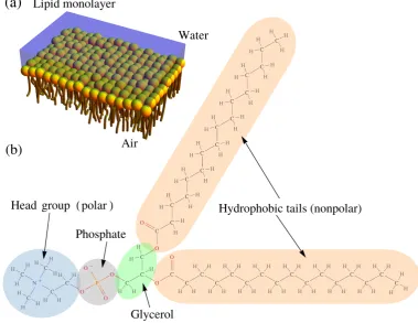
1.1 Schematic diagram of lipids which form a Langmuir monolayer at a water-air interface, and the structural formula of a single lipid. . . . 3

1.2 Diagram of the lipid bilayer structure according to the model

pro-posed by Gorter and Grendel. . . 4 1.3 A three-dimensional representation and cross-sectional views of a

bi-ological membrane in a modern perspective of thefluid mosaic model

originally proposed by Singer and Nicolson. . . 6

1.4 The chemical structure of some common membrane lipids. . . 8

1.5 Structures of micelles formed by amphiphilic molecules. . . 11 1.6 Schematic picture of a lipid hexagonal phase, and a cross-sectional

view of a lipid aggregate in the inverted hexagonal phase. . . 12

1.7 Schematic illustration of lipid molecules forming a lamellar phase, and a diagram of a uni-lamellar lipid vesicle. . . 13

1.8 Schematic diagram of the phases within a lipid bilayer. . . 17

1.9 Rotations about a C–C bond in a fatty acid chain produce different conformations, the so-calledtrans-gauche isomerisations. . . 18

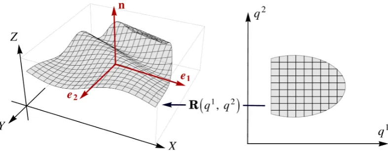
2.1 Sketch of the surface parametrisation, where a region in the q1q2 -plane is mapped to a two-dimensional surface embedded in a three-dimensional spaceR3 through a real vector functionR(q1, q2). . . . 21

2.2 Illustration of a saddle surface embedded inR3, displaying the

prin-cipal directions of a point on the surface. . . 23 2.3 The Monge parametrisation of a two-dimensional surface, namely a

surface described by a height functionu(x, y) above thexy-plane. . . 26 3.1 Schematic diagrams of a single transmembrane protein embedded into

a two-component fluid membrane composed by lysophospholipids and

(7)

3.2 Schematic diagram of the membrane-inclusion model. Here, the

sur-face of the membrane in the vicinity of a membrane protein is de-scribed in the Monge parametrisation byu(r, θ), wherer is the radial distance from the center of the protein, andθ is the azimuthal angle. 44 3.3 Plot of k±2 against γ, which shows that both k+ and k− are real for

γ <|α−β|, and purely imaginary forγ > α+β. . . 48 3.4 Radial profiles of the the mid-plane of the bilayeru(r) and the

com-positional asymmetry φ(r), which are induced by a rigid membrane inclusion with a small contact angle. . . 57

3.5 Membrane deformation profiles induced by an asymmetrical

inclu-sion, e.g. LeuT. The surface heights represent the mid-plane of the bilayer for different values of the widthw, which gives the asymmetry in the contact angle at the protein-membrane interface. . . 59

3.6 Total membrane deformation energy, for various values of the cou-pling term γ, against the width w, where the phase ζ = 0 and the magnitude of the contact angle is set to beδ0 = 15◦. . . 60 3.7 Diagrams of two idealised gating schemes for mechanosensitive

chan-nels, namely the dilational model, and the gating-by-tilt model. . . . 61

3.8 The estimated angle for the gating-by tilt that accounts for the total conformational energy change as measured for MscL and MscS. . . . 62

3.9 Schematic diagram of a biomembrane deformed by the assembly of a

protein coat. . . 62 3.10 The free-energy per unit area of coat monomers (that is purely due to

the curvature coupling to the compositional variations) as a function

of the radius of the projected coat area. . . 64

4.1 Schematic diagram of a three-dimensional membrane patch of a

quasi-spherical lipid vesicle (depicted here by the blue region), and a

two-dimensional cross-section along the xz-plane. The latter illustrates the shape fluctuations of the vesicle about a fixed radius R, which are given byu(θ, ϕ), with ϕ= 0 in this case. . . 67 4.2 Schematic diagram of a fluctuating vesicle, where the light-blue plane

illustrates the focal plane of the microscope, whilst the green slab

depicts the region within the focal depth ∆ of the objective, where

(8)

4.3 Schematic diagram of the intensity field I(r, ϕ) at the focal plane, which corresponds to the projected membrane surface within the focal depth of the objective (red indicates high intensity, while blue is low).

The solid black line represents the first radial moment of the intensity,

namelyρ∆(ϕ)∝

R∞

0 rI(r, ϕ) dr. . . 75 4.4 Log-log plot of the mean squared amplitudes

|µˆq|2

as a function of

the azimuthal mode numberq for some values of the focal depth ∆. 78 4.5 The fluctuation spectrum for a GUV of mean radius R ≈ 23 µm,

which is imaged by using a confocal fluorescence technique. . . 81

4.6 Data representation of a single GUV of mean radius R= 10.2 µm, which is observed under a confocal microscope (with τ ' 1 ms the inverse scanning rate). The inferred values of the bending modulusκ from the fluctuation spectra of the vesicle individually measured at

different focal depths ∆. . . 84

5.1 Raft removal rate in the recycling scheme (5.2) for various values of

λc, where the dimensionless size s = a ω, and the rescaled outward

fluxesJoff = joff/(ω D) = 1 and Foff =foff/(ω D) = −0.95 (dashed lines) and +0.95 (solid lines), with the same colour convention. This illustrates that the model (5.2), depending on the sign of Foff, can account for both recycling at small and large scales. . . 89

5.2 Plots of the total number-per-area of domains ρ(τ) and their area fraction φ(τ). The initial boundary conditions at τ = 0 are given by the following step-like changes: 50% decrease inJoff (blue); 50% decrease inJon (red); and 50% decrease in bothJon and Joff (green). 93 5.3 Log-log plot of the the steady state value of the dimensionless mean

domain sizeA:=φ∞/ρ∞ as a function of the recycling strength at a fixed area coverage. . . 94

5.4 Log-log plot of the domain size distribution in Laplace space for the size-independent case (green curve) and the size-dependent case (blue

curve), where the parametersλc= 0.01,Jon= 10−5,Joff= 10−4, and Foff = 10−1. The red dashed line shows the steady-state solution of the Pad´e approximant in equation (5.67). The inset plot displays the

(9)

Acknowledgments

Usually a full paragraph of acknowledgements is included in a rather short

four-page article that is published in the Physical Review Letters journal. By a simple

scaling argument, this might naively suggest that I need to write here almost 30–40

paragraphs of acknowledgements. Since I am not willing to use this much space,

for the sake of brevity (but also for the sake of my sanity!), I would like to use this

opportunity to express as short as possible my sincere appreciation to a number of

people that supported me and helped make this thesis possible.

Firstly, I would like to acknowledge both my supervisor, Matthew Turner,

and George Rowlands, to whom I extend my heartfelt gratitude for their huge

sup-port throughout my doctoral studies, as both teachers and close friends. Notably,

they have guided me with great patience, whilst also being hard working and

metic-ulous. Above all, they have always acted with warmth and friendliness towards me

which has helped making my research at Warwick very enjoyable. Also, thanks for

all the casual and interesting conversations that we had over a couple of good beers

in the famous Virgins and Castle (notoriously known for the game of spoof).

Secondly, I owe a debt of gratitude to Nina, Alex, Steph, and all the guys

of PS.001, including Dan, Andy, Matt, Edu, Jack, Erick, and Anja. Thanks for

your friendly support and all the laughs, and more importantly thank you for the

numerous discussions ranging from utter silliness to refreshingly insightful topics.

Last but not least, I would like to thank my family for their best wishes and

constant encouragement. In particular, I would like to give a special thanks to my

eldest brother, Lucian, for his tremendous support throughout my life, for which I

(10)

Declarations

I hereby declare that my thesis entitled Physics of Biomembranes is the result of

my own work, unless stated otherwise. This thesis is submitted to the University

of Warwick as my application towards the degree of Doctor of Philosophy. It has

been composed by myself and no part of this thesis has been submitted for a degree

at any other university. This work has been carried out under the supervision of

Prof. Matthew S. Turner and Prof. George Rowlands at the University of Warwick

from October 2011 to April 2015. The following research work has been submitted

to refereed journals for publication:

1. S. A. Rautu, G. Rowlands, and M. S. Turner, Membrane Composition

Variation and Underdamped Mechanics near Transmembrane Proteins

and Coats, Phys. Rev. Lett.114, 098101 (2015)

2. S. A. Rautu, D. Orsi, G. Rowlands, M. S. Turner, and P. Cicuta,The

Role of Optical Projection on Vesicle Fluctuations [In preparation]

3. S. A. Rautu, G. Rowlands, and M. S. Turner, Size-dependent

(11)

.

. .

. . .

“The road to wisdom?–Well, it’s

plain and simple to express:

Err

and err and err again,

but less

and less

and less.”

(12)

Abstract

The basic building blocks of all biomembranes are lipid molecules, which

self-assemble to form a very thin and stable barrier, where a variety of proteins

can be incorporated into its structure. These two-dimensional systems exhibit a

plethora of physical phenomena, which are an abundant source of inspiration for a

physicist. The physical aspects of biomembranes are described within a

phenomeno-logical model, the so-called Canhan–Helfrich theory, which relies primarily on the

geometrical aspects of the membrane surface at large scales.

Using this theory, we study the response of a membrane to the inclusion of a

transmembrane protein or a protein coat by coupling the composition to the mean

curvature. A transition is found from an overdamped to an underdamped regime for

the membrane shape and its compositional variation. This leads to large membrane

undulations near the inclusion, resulting in the activity suppression of

mechanosen-sitive channels and a preference for the formation of protein coats.

We also re-examine the methodology for inferring the bending modulus of

membranes from their observed thermal fluctuations. Particularly, we analyse the

effect due to the optical projection of such shape undulations across the focal depth

of the microscope. A comparison of this with the literature approaches reveals a

systematic decrease in the value of the bending modulus, resolving a previously

recognised discrepancy between shape measurements and other known techniques.

Lastly, we investigate an non-equilibrium model for the formation of

mem-brane domains that also involves memmem-brane recycling. The dynamics and the

steady-state features of the domain size distribution are analytically revealed and the

(13)

Chapter 1

Introduction

The research area of biomembranes has become an important interdisciplinary meet-ing point for various fields of science and technology rangmeet-ing from applied

mathe-matics to nano-medicine. There are very good reasons for its wide appeal and

in-terest. Firstly, its biological significance: each living cell, including their organelles, is bounded by a sac-like membrane that plays an active and crucial role in almost

every cellular process. Membranes spatially separate intracellular compartments

and define a boundary with the extracellular medium [1]. This compartmental-ization is fundamental for an organism, allowing highly specialised functions [2].

Hence, a complete knowledge of membrane phisicochemical properties is essential

for understanding the diverse phenomena observed in cells, which are the building blocks of all living matter. A few examples include the selective transport of ions across membranes through protein channels [3], regulation of the response to osmotic

shock [4–6], cellular transport, signal transduction, cell adhesion, DNA replication, protein biosythesis [7], and the flow of red blood cells through narrow capillarities [8].

Many important medical problems also involve membranes, such as understanding

the nerve pulse conduction and the mechanism of general anaesthesia [9]. Moreover, much of the recent effort in drug development concerns with the design of specific

molecules that target the activity of proteins present in membranes. Approximately

one third of all proteins are membrane resident, and these are the targets of about 60% of all currently approved drugs [10]. Another motivation is biomimetics and

the use of membranes for constructing biotechnological applications, including

drug-delivery systems [11], miniature chemical reaction vessels [12], and biosensors that combine electronic devices with membranes [13]. Biomembranes are therefore of

(14)

The reasons for studying biomembranes from a purely physical point of view

are that living systems, such as cell membranes, have to abide by the same laws of physics as inanimate objects. However, biological materials are extremely

com-plex systems (usually, out of equilibrium), with non-trivial properties that are often

specific rather than generic [14]. Despite this complexity the physical properties of biomembranes can be studied within a thermodynamic framework using

course-grained models that span specific spatial and temporal scales [15]. Interestingly,

the characteristic energies identified in biomembranes (for example, the aggregation energy per monomeric constituent) are typically an order of magnitude larger than

the thermal energy (namelykBT, wherekBis Boltzmann’s constant andT ≈300 K

is the room temperature). As a result, biological membranes are usually found to be stable against thermal fluctuations at physiological relevant temperatures, but also

sufficiently soft so that they can be readily deformed by membrane proteins or other

biochemical processes [14–16], e.g. ATP hydrolysis [1,2]. Their ability to bend under very low stress is one of the main mechanical properties of membranes. This feature

can be easily observed under an optical microscope, where the thin wall of cells is

found to fluctuate (the so-called flicker phenomenon) [14]. Another attractive reason for a physicist to study biomembranes is because of the separation of scales, that is,

the thickness of membranes is much smaller than their lateral extent. This allows us to model membranes as two-dimensional systems, reducing the dimensionality of

the problem in the limit of large scales (see [15] and [16] for a detailed review). By

exploring biomembranes in this way, we can attain general insights into the physical properties of cell membranes and their associated phenomena, such as scaling laws,

and more importantly how these findings may couple to particular biological

func-tions. Therefore, biological membranes provide an abundant source of inspiration to both physicists and applied mathematicians.

1.1 Historical Perspective

The current picture of biological membranes is a legacy of nearly a century of scien-tific research. Thus, in order to introduce the basic constituents of a membrane, as

well as the orders of magnitude of the relevant physical quantities, a short history

about the discovery of the membrane structure and its composition is presented in this section (see [7], [9], [14], and [17], where a number of reviews on the history of

biological membranes is discussed in great detail).

Arguably, the physics and chemistry of biological membranes began with

(15)

[image:15.595.99.479.210.503.2]

(16)

investigated the permeability of cell membranes for various compounds [18]. It was

observed that cells are enclosed in a selectively permeable barrier, and fat-soluble molecules are more likely to penetrate it than water-solvable molecules or ions [17].

Overton’s findings led to the speculation that membranes have similar properties to

oils, being a lipid of some sort, which nowadays is known to be rich in cholesterol and phospholipids [2] (their composition is discussed in more details in Section 1.2).

Figure 1.2: Diagram of the lipid bilayer

structure according to the model

pro-posed by Gorter and Grendel [20]. In a seminal paper published in

1917, Irving Langmuir provided a sim-ple technique for measuring the lateral

pressure exerted by a lipid membrane as

it spreads at a water-air interface [19]. Using the proposed apparatus, which is

known as the Langmuir trough, he was

able to show that lipids form a closely packed mono-molecular layer on the

sur-face of water, where the area per lipid

was found to be about Alipid = 0.7 nm2.

Langmuir also suggested the amphiphilic

nature of these molecules, as shown in Figure 1.1 (a). Amphiphiles are molecules

made of a polar hydrophilic head group,

possessing high affinity for water, and one (or two) hydrophobic hydrocarbon tail(s), which has (have) a low affinity for water – see Figure 1.1 (b).

In 1925, using Langmuir’s methods, E. Gorter and F. Grendel revealed that

the membrane structure of erythrocytes (or red blood cells) is a lipid bilayer [20], where the hydrophobic part of the molecules is isolated from water by the layers

of hydrophilic heads (see Figure 1.2). This was achieved by dissolving the lipids

using acetone, then measuring the surface area of the extracted lipids in a Langmuir trough, and lastly comparing this value with the area of dried red blood cells.

How-ever, their studies included two errors: acetone does not extract all the lipids, but

this error was compensated by their error in measuring the surface area of erythro-cytes [7, 9]. Nonetheless, their experiment concluded that the ratio of surface area

occupied by lipids to the area of the cell is approximately two, a number consistent

with the theory that cells are enveloped by a lipid bilayer structure [17]. Or, in the words of the pioneering study [20]:

“ [...] all our results fit well with the supposition that the chromocytes

(17)

This bimolecular configuration forms the basic structure of all biomembranes, and

represents the predominant structure out of the large conformational polymor-phism exhibited by amphiphiles [14]. Namely, a mixture of water and amphiphilic

molecules can generate a broad diversity of thermodynamically stable phases besides

the lamellar phase illustrated in Figure 1.2 (see Section 1.3 for further details). In the 1930s, H. Davson and J. F. Danielli [21] elaborated a new membrane

model, where both sides of the lipid bilayer are coated by a layer of proteins, in

order to explain the measured differences in the permeability (of ions or other apo-lar molecules) between an artificial membrane and the plasma membrane found in

cells [14]. This selective permeability was hypothesised to be governed by

electro-static interactions and membrane potential. The Dawson–Danielli unit membrane model was the first commonly accepted model, dominating the membrane research

in the subsequent years, and undergoing only minor changes in the 1950s due to

the advent of electron microscopy [17]. The latter allowed the structure of mem-branes to be directly imaged, primarily through the works of J. D. Robertson [22],

who discovered that the plasma membrane and all cell-organelle membranes (e.g.

membrane of the cell nucleus, the Golgi apparatus, and the double layers of mito-chondria) have a common construction principle, supporting the previous models

introduced by Gorter and Grendel, in 1925, and Davson and Danielli, in 1935 [9]. Moreover, direct and indirect measurements of the membrane thickness (through

electron micrographs and X-ray diffraction techniques, respectively) yield a value

on the order of 5–8 nm, with a hydrophobic core of about 3–4 nm [14].

The next major phase in biomembrane research arrived in the late 1960s,

when numerous studies [23], involving freeze-fracture electron microscopy methods,

determined that proteins do not cover the bilayers, but they form globular particles, which are embedded within the membrane [7]. At the same time, with the rapid

development of magnetic resonance methods (such as, nuclear magnetic resonance

and electron spin resonance), many experiments showed that lipids can move lat-erally in the plane of the membrane [24], with a characteristic diffusion constant

given by D_lipids ∼ 10−8 cm2/s ≈ 106A_lipid/s [14], revealing the fluid nature of biomembranes [17]. Some proteins were also found to freely diffuse in the lipid bi-layer, with a diffusion constant that is much smaller than that of lipids: typically,

Dproteins ∼10−10 cm2/s = 10−2Dlipids [14]. Furthermore, the asymmetry between

the inner and outer layer of membranes was established, and the notion of trans-membrane proteins was confirmed, being firstly observed on red blood cells, where

(18)

[image:18.595.94.487.207.487.2]

(19)

This research culminated in thefluid mosaic model of biomembranes (1972), also known as the Singer–Nicolson model [26], which describes a membrane as a fluid (that is, the lipidic bilayer made of various phospholipids and cholesterol) in

which other macromolecules are incorporated, such as peripheral (adsorbed on the

membrane surface) and integral (embedded in the bilayer) membrane proteins, as shown in Figure 1.3. The proteins act as active components and provide a variety of

biological functions, including cellular transport, adhesion and signalling [1, 2]. As

a loose comparison, the lipid bilayer became the arctic sea in which various icebergs (proteins) can float freely. Interestingly, the lipid-to-protein ratio varies significantly

across different biological membranes; for example, the inner mitochondrial

mem-brane is approximately 76% protein, while the myelin memmem-brane is only 18% [7]. Although the Singer–Nicolson model is a major influential step in the study of

biomembranes, integrating various experimental findings from the preceding decade

on the physics and chemistry of membranes, many refinements have been amended over the past years [17, 27]. We now know that the bilayer is a highly dynamic

sys-tem, where the lipids and proteins are not homogeneously distributed, but they form

domains and clusters [9]. In particular, intermediate-sized domains with a diameter between 10–100 nm (and rich in sphingolipids and cholesterol) have been proposed

in biomembranes – the so-called lipid raft hypothesis – to explain the problem of sorting and trafficking lipids and lipid-anchored proteins [28, 29]. This phenomena

is discussed in much more detail in Chapter 5. Another amendment is due to the

hydrophobic matching: if the hydrophobic core of the membrane is longer or shorter than the hydrophobic belt of the embedded protein, this leads to membrane

thick-ness deformations [30]. Either the protein deforms to the match the thickthick-ness of the

bilayer or the adjacent lipids stretch to compensate for this hydrophobic mismatch, or both. This effect results in non-trivial protein-lipid interactions as well as

lipid-lipid interactions [31–35]. Membrane curvature is also an important key concept,

which can drive lipid sorting and membrane mediated interactions [36, 37]. This is explored in more details in Chapter 3. Lastly, another interesting aspect concerns

the presence of specific lipids in the vicinity of proteins in order to regulate their

biological function. Arguably, this might be one of the reasons for the very large number of lipid species present in biological membranes (on the order of thousands);

(20)

[image:20.595.92.491.105.335.2]

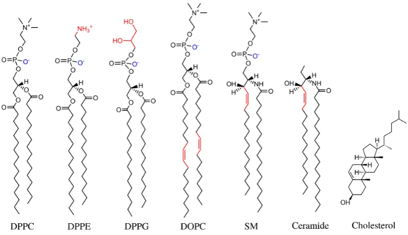
Figure 1.4: The chemical structure of some common membrane lipids. Three phos-pholipids with two palmitic chains are shown, where the head groups are given by phosphatidylcholine (DPPC), phosphatidylethanolamine (DPPE), glycerol (DPPG), as well as a phospholipid with two oleic chains and a phosphatidyl-choline head group (DOPC). Some lipids without phosphate groups are also shown, such as sphingomyelin (SM), ceramide, and cholesterol.

1.2 Membrane Lipids

The macromolecules found in biological systems can be classified in four main classes:

the carbohydrates, the fats, the proteins, and the nucleic acids [1]. Out of all these

types, the fats (e.g. lipids) are the only one that do not form polymers, but instead they self-assemble into aggregates in an aqueous solution (e.g. water), leading to a

variety of structural phases [7]. This behaviour is due to their amphiphilic nature,

namely they are made up of a hydrophilic head group and a hydrophobic region [14]. Despite this simple construction principle, the compositions of both the hydrophilic

groups and the hydrocarbon chains display a large variation, giving raise to a zoo

of numerous types of lipid species (several thousands) [9]. To put this number into a biological perspective, the alphabet of possible lipid mixtures in biomembranes hugely exceed the 4-letter alphabet used to identify the nuclei acids, as well as the

20-letter alphabet of the amino acids that describe proteins [38].

Out of this plethora of lipid species, phospholipids are the most abundant

type [2, 7]. Their molecular structure consist of two fatty acids that are covalently

(21)

Name Chain length:

number of double bonds Position of unsaturations

Lauric 12:0 –

Myristic 14:0 –

Myristoleic 14:1 –

Palmitic 16:0 –

Palmitoleic 16:1 9-cis

Stearic 18:0 –

Oleic 18:1 9-cis

Linoleic 18:3 6-cis, 9-cis, 12-cis

Arachidic 20:0 –

[image:21.595.114.468.110.296.2]

Aracidonic 20:4 5-cis, 8-cis, 11-cis, 14-cis

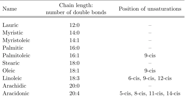
Table 1.1: A selection of common saturated and unsaturated fatty acids that form the hydrocarbon chains of lipids. Adapted from [9].

turn, is linked (through the third position) to a negatively charged phosphate group

that carries the terminal polar head [7]. The latter group can be composed by various organic compounds, such as choline, ethanolamine, serine, inositol, or even

glycerol (see Figure 1.4 for some examples of their chemical structure) [7]. There

is also an enormous range of possible fatty acids, which can vary by chain length and degree of saturation [9] (see Table 1.1 for the most common fatty acids found in

nature). The typical hydrocarbon chain length is most frequently an even number

between 12–20, but chains as short as 8 carbon atoms have also been found in some bacteria [39]. Furthermore, most of the hydrocarbon chains are unsaturated, where

several double bonds between the carbon atoms are present along the chain. This number represents the degree of saturation, and it is typically between 1–3 (see

Table 1.1). Lipid molecules that have only single bonds are known to be saturated.

As a consequence, a sophisticated (and also relatively intimidating) termi-nology has been developed to efficiently describe the structural form of

phospho-lipids [7]. For example, the lipid molecule shown in Figure 1.1 (b), which has a

choline head group and two palmitic chains, is named 1,2-dipalmitoyl-sn-glycero-3-phosphocholine. This is usually abbreviated as DPPC, using a common four-letter

(22)

1-palmitoyl-2-oleoyl-sn-glycero-3-phosphoethanolamine is shortened as POPE.

There are many other ways of making lipids: for example, the glycerol back-bone can be replaced by a sphingosine, which belongs to the family of amines [38].

The simplest version of this molecule is ceramide, as shown in Figure 1.4. Since this

is a purely hydrophobic compound, a hydrophilic head can be attached in principle, which leads to variety of other lipids, e.g. sphingomyelin, if the head group is a

phos-phatidylcholine [38]. These lipids often occur with long saturated tails (24 carbons)

and they are believed to play a role in the formation of microdomains (or rafts) in biomembranes [9]. Another important example is cholesterol, which is a member

of the steriod family and it is ubiquitous in the membrane of eukaryotic cells [39].

Instead of a fatty-acid chain as its hydrophobic region, the cholesterol has a steriod ring structure, and its hydrophilic polar head is simply given by a small hydroxyl

group -OH [7], see Figure 1.4. Interestingly, the cholesterol is known to influence

the membrane fluidity [14], increasing the viscosity in the fluid phase (where the lipids diffuse freely and their hydrocarbon tails are disordered), while decreasing

the melting temperature (we shall discuss this in more details in Section 1.4).

Not surprisingly, this chemical variability makes lipids the most diverse group of molecules found in cells. The reason for this striking feature is still an open

ques-tion, although there is an increasing understanding of the collective and functional role of lipids in biomembranes [38, 39]. For a fuller account on the classification of

the membrane lipids, the reader is referred to [2] and [7].

1.3 Self-assembly of Lipids

Due to the hydrophilic effect, the lipid molecules self-assemble into many possible

super-molecular structures [2], see Figures 1.5–1.7 for a few examples. In other

words, in a mixture of water and lipid molecules, the system tends to minimise the free-energy by shielding the hydrocarbon chains from the water, with larger

assem-blies more favourable at higher lipid concentrations [2, 9]. The self-assembly process

also depends on the other intensive thermodynamic variables of the system, such as the temperature, the ambient pressure, or the chemical potentials of solvents [9].

Micelles occur when the solution is sufficiently dilute, such that the

concen-tration of lipids is above some critical value that is known as the critical micelle concentration [9]. In a micelle, all the hydrophobic tails point radially towards

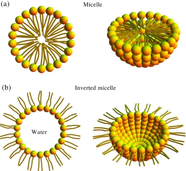
each other, and their hydrophilic parts form a sphere-like surface, as shown in Fig-ure 1.5 (a). Inverted micelles can also be generated where the hydrocarbon chains

(23)

[image:23.595.101.481.215.563.2]

(24)

[image:24.595.103.482.142.633.2]

(25)

[image:25.595.93.491.112.363.2]

Figure 1.7: (a) Schematic illustration of lipid molecules forming a lamellar phase, namely a stack of bilayer units which are seperated by a water layer. (b) Diagram of a uni-lamellar liposome, also known as a lipid vesicle.

see Figure 1.5 (b). The formation of inverted micelles occurs at very low water

concentrations, or in an oil-water mixture when the amount of water is small [2].

If the lipid concentration is increased even more, there is generally a transi-tion from the configuratransi-tion of spherical micelles to other geometries, such as

cylindri-cal aggregates ordered in a hexagonal arrangement (known as the hexagonal phase),

see Figure 1.6 (a), where the spacing between the micellar cylinders varies between 1–5 nm depending on the relative concentration [2]. An inverted hexagonal phase

can exist, which is exactly the same as the hexagonal phase, but with the apolar

chains radiating outwards from the cylinders that enclose the water. Typically, the diameter of these inner cylinders is about 1–2 nm [2]. However, the exterior space

is completely filled by the hydrophobic chains, as shown in Figure 1.6 (b), and thus the spacing between cylinders is much smaller than in the hexagonal phase.

Moreover, a range of cubic crystal phases with a periodic three-dimensional

order are possible, which can be formed, as before, in a water-continuous manner or in a hydrocarbon-chain-continuous manner [2]. The simplest cubic phase is given

by a cubic arrangement of small aggregates, such as spherical micelles or inverted

(26)

arrange-ments are composed by a large continuous network of channels, which can be either

water continuous or apolar chain continuous [2]. Another interesting phase, which is usually found in detergent systems and possibly in some lipid systems, is the sponge

phase. This topologically mimics a bicontinuous cubic phase, but it does not display

any periodic three- or two-dimensional structure [9].

Lastly, the simplest and also the most ubiquitous lipid phase found in nature

is the lamellar phase, see Figure 1.7 (a), which includes single bilayers or

multi-layered arrangements of bilayers that are stacked on top of each other, and spaced by a water layer with a thickness of about 1–10 nm [2, 39]. Evidently, open ends are

energetically very costly due to the exposure to water, and hence the bilayers and

multi-lamellar bilayers normally close onto themselves, forming closed structures, see Figure 1.7 (b), which are typically referred as uni-lamellar and multi-lamellar

liposomes (or lipid vesicles) [39], respectively. Vesicles, either uni-lamellar or

multi-lamellar, are stable on a time-scale of days [15] and they can be artificially produced in the laboratory (a review of the preparation techniques can be found in [40]).

These vesicles, which can be made from a few lipids and membrane proteins, are

essential for the physical, life, and biochemical sciences as they represent a simplified model of a cell membrane, where specific biological functions of the membrane can

be investigated on a molecular level [39].

Although we introduced the various aggregate structures as a function of the

lipid concentration, this is by no means the only control parameter that determines

the equilibrium phase and its stability. As previously mentioned, the self-assembly mechanism into different aggregates depends sensitively on temperature, chemical

structure and other environmental conditions [9] (e.g. a temperature increase can

lead to a crossover transition from a lamellar structure into an inverted hexagonal or cubic structure [39]). This leads to a high dimensional phase space with a very

complex phase diagram, where different regions support a particular structure of

lipid assemblies (see [2] for a complete review).

Remarkably, many of these factors can be described qualitatively within a

very simple framework that involves only the effective molecular shape of a lipid

molecule [38]. However, it is important to emphasise that a lipid incorporated into an aggregate does not occupy a well-defined volume, as there are no hard edges on

this length scale [39]. This effective molecular shape can be related to the mean

cross-sectional area a and the volumev that a lipid would occupy on average, and also how deeply it is embedded in the lipid aggregate, say `. These parameters are influenced by numerous geometrical constraints, such as the size of the polar head,

(27)

affects the configuration of the hydrocarbon chains, as the presence of double bonds

causes kinks in the usual linear arrangement of the carbon atoms (that is, all-trans, see Section 1.4). Moreover, the temperature leads to rotational excitations around

the C–C bonds and, as a result, increases the area occupied by the hydrocarbon

tails [7]. This effect causes membrane melting transitions [9], which are discussed in more details the following section. In addition, the charge and the hydration of

the head groups can also contribute to the phase preference [41] and hence to the

effective shape of the lipid molecule [39].

The consequences of the effective molecular shape of a lipid has been

stud-ied by Israelachvili, Mitchell, and Ninham in a famous paper from 1976 [42], which

to a physicist it is a marvellous example of the power of simple geometrical argu-ments. The ability of a lipid to fit into a specific aggregate is described by a packing

parameter P, which is given by

P = v

a `, (1.1)

where a, v, and ` are defined above. Since micelles are spherical aggregates, their total area and volume can by computed through the equations N a = 4πR2_m and N v = 4πR3_m/3, respectively, where Rm is the radius of the micelle and N is the

number of lipid molecules in that spherical aggregate. Since the length ` of the individual lipids needs to be at least greater than the radiusRmfor packing reasons,

namely `≥Rm, we find that the parameterP must be smaller than 1/3 in order to

produce stable spherical aggregates. For a cylindrical aggregate of radius Rc and a

very long length LRc, we have two similar equations for their area and volume,

that is, N a = 2πLRc and N v = πLRc2, which yields that P ≤ 1/2 since ` ≥ Rc

must hold as before for closed packing. However, we already know that if P ≤1/3 this leads to the formation of micelles. Thus, the stability condition for cylindrical aggregates is given by 1/3≤P ≤1/2. By repeating the same argument for planar or lamellar structures, the condition required for stable lipid bilayers can easily be derived, namely 1/2 ≤ P ≤1. Moreover, as the volume v of a cylindrical-shaped lipid is exactlya`, then values ofP >1 suggest an effective molecular shape in form of an inverted cone, and cubic and inverted non-lamellar phases can be expected [39]. Interestingly, lipids extracted experimentally from real biological membranes,

which are typically multi-component systems and appear to be in the lamellar phase,

often self-aggregate into non-lamellar structures when suspended in water, regardless of whether they were removed from various different organisms or different types of

cells from the same organism [38,39]. This suggests that many of the lipids present in

(28)

membrane proteins, local membrane composition, or by budding of the membrane

in exocytosis and endocytosis processes [38]. The former two examples are explored in more details in Chapter 3, where the role of membrane compositional asymmetry

near a trasmembrane protein is analysed within a continuum model.

1.4 Membrane Melting

Throughout the rest this thesis, we study only one of the phases mentioned above,

namely membranes in the lamellar phase and formed by a single bilayer. However, the lipid order within a bilayer passes as well through different states, which depend

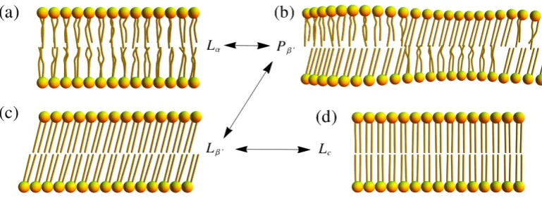
primarily on the temperature [9]. The following lipid phases can be found in bilayers

and they are listed below in terms of their occurrence at decreasing temperature:

• Fluid phase (Lα): This phase occurs at high temperature [2], where the lateral

distribution of lipids is rather random, and all their hydrocarbon tails are rather disordered (fluid-like). This phase is believed to represent the typical

bulk of biological membranes.

• Ripple phase (Pβ0): The surface of the bilayer displays ripples, or wave-like structures, which can be observed in electron micrographs [7]. This phase consists of a binary mixture of lipids in Lα and Lβ0 phases (see below) that are most often arranged in an one-dimensional periodic structure [9].

• Gel phase (Lβ0): The lateral distribution of lipids shows a two-dimensional triangular lattice, and their fatty acid chains are mainly ordered in the all-trans

configuration (see Figure 1.9) and tilted with respect to the membrane normal

(hence, use of the prime symbol in its short notation) [9]. This tilt is due steric

effects, that is, a mismatch between the head groups and hydrophobic tails, which does not allow the lipids to be stacked parallel to the normal [43].

• Crystalline phase (Lc): This occurs at much lower temperatures, and it is

sim-ilar to the gel phase, expect there is no tilt angle [9]. Moreover, this is usually

characterised by a three-dimensional order of a multi-lamellar configuration of lipids, where the water layer is completely absent [2].

These phases are illustrated in Figure 1.8. The crossover transition between these

four phases occurs at well-defined transition temperatures, which mostly depend on

(29)

[image:29.595.95.480.105.246.2]

Figure 1.8: Schematic diagram of the phases within a lipid bilayer, where the temper-ature decreases from (a) to (d). Namely, the fluid phase (Lα), the ripple phase (Pβ0), the gel phase (Lβ0), and the crystalline phase (L_c), respectively. The conformational ordering of the hydrocarbon chains increases as the temperature drops.

The transitions Lβ0 ↔ P_β0 and P_β0 ↔ L_α are known in the biomembranes literature as the pre-transition and main-transition [2], respectively. They are both

fundamentally controlled by the hydrocarbon chain melting process. Namely, rota-tions about C–C bonds in a saturated chain result in three distinct energy minima

that correspond to different conformations (or isomerisations), so-called gauche−,

trans, and gauche+ [7], as illustrated in Figure 1.9. The trans isomer is the most stable, being the global energy minimum, and a chain configuration with all

sin-gle carbon–carbon bonds in this state (i.e. all-trans) yields a hydrocarbon tail that is maximally extended [39]. At high temperatures every isomer is equally proba-ble, and therefore the chain conformation becomes more disordered, disrupting the

crystalline structure of the lipid bilayer. The melting temperatures (namely, the temperatures at the pre-transition and main-transition) are higher as the length of

the chain is longer [9]. However, the presence of double cis bonds∗ greatly reduces the melting point [9]. As an example, the melting temperature (of the main tran-sition) of DSPC is around 53oC, whilst DOPC has a much lower melting point,

about −20oC, although the difference between the lipids is only an extra double bond in DOPC [9]. Therefore, saturated lipids melt at considerably higher tem-peratures (i.e. they are easier to order) than lipids with unsaturated chains which

have permanent kinks. This effect is used by a variety of organisms that adjust

their membranes to function at lower or higher temperatures (or even at different ambient pressures) [9].

∗

(30)

[image:30.595.101.482.107.305.2]

Figure 1.9: Rotations about a C–C bond in a fatty acid chain produce different conformations, the so-called trans-gauche isomerisations. This leads to three local minima seperated by 120o, namelygauche−,trans, andgauche+, which correspond to the orientations shown above each minimum in a Newman projection diagram. The chain configuration with all of its C–C bonds arranged in the trans isomer has the lowest energy state, corresponding to a zig-zag arrangement of the carbon atoms. The other two gauche configurations are mirror images of each other, and they have a higher potential energy than thetrans isomer. Adapted from [7].

The addition of cholesterol in lipid bilayers has a dual effect, namely, it en-courages the close packing of the hydrocarbon tails in theLαphase, while it disturbs

the chain ordering in the Lβ0 phase [39]. Thus, in a mixture of lipid molecules and cholesterol, a liquid-ordered phase (Lo) and a liquid-disordered phase (Ld) appear

when the concentration of cholesterol is found in large (& 40%) and moderate

amounts [44], respectively. In the former phase, the hydrophobic tails are relatively

ordered, but the membrane still preserves its fluidity. Thus, a membrane in the

liquid-ordered phase behaves as a fluid with translational disorder and high lat-eral mobility, decreasing as a result the melting temperature [2]. Furthermore, the

high concentration of cholesterol makes the thickness of the membrane larger and also less flexible [39]. On the other hand, the Ld phase is equivalent, in fact, with

the previously introduced Lα phase, where its fatty acid chains are less ordered in

comparison with the Lo phase (in terms of both translational and conformational

degrees of freedom) [2, 39]. In a binary mixture of Lo and Ld phases, the minority

phase normally forms domains due to phase separation [45]. The phenomena

(31)

interest is motivated by the appealing theoretical challenges that are ingrained in

this system, but also by the aspiration to gain physical insights into the nature of lipid rafts observed in membrane cells. This is discussed more in Chapter 5.

1.5 Outlook

The fundamental building blocks of all cell membranes are lipid molecules, which self-assemble to form a very thin and stable barrier where a multitude of proteins

can be incorporated. In addition, they exhibit a wealth of physical phenomena including self-assembly, phase transitions, domain formation, and many other

dy-namical processes. For a physicist, the challenges are to understand and model these

phenomena, and to generate testable predictions which can be then compared with data from biological experiments.

In this thesis, we focus on a number of problems concerning the mechanical

and dynamical properties of fluid membranes, namely lipids organised in a bilayer that display a liquid-crystalline phase. On length scales larger than the membrane

thickness, they can be treated as two-dimensional elastic sheets whose equilibrium

shape and thermal fluctuations are only controlled by a handful of coarse-grained material parameters. The physical and mathematical aspects of this description are

presented in Chapter 2, which is structured as follows: firstly, we present the

essen-tial differenessen-tial geometry of two-dimensional surfaces; secondly, we show how these geometrical tools can be used to describe a fluid membrane through the so-called

Canhan–Helfrich theory; and, lastly, we review some of the experimental studies

carried out to estimate the phenomenological parameters in this model. Using this theory, in Chapter 3, we develop a model for the response of a fluid membrane, in

terms of composition and shape, to the inclusion of a rigid transmembrane protein or

a protein coat. In Chapter 4, we re-examine the methodology for inferring mechan-ical information about membranes from their observed fluctuations and dynamics.

Particularly, we analyse, within a Gaussian approximation, the effect produced by

the optical projection of surface modes across the focal depth of the microscope. In Chapter 5, we study an out of equilibrium model for the kinetics of the spontaneous

membrane raft formation via membrane recycling. Finally, Chapter 6 summarises

(32)

Chapter 2

From Differential Geometry to

Fluid Membranes

Fluid membranes have a clear separation of scales, namely the thickness of lipid

bilayers (about 5 nm thick) is typically several orders of magnitude smaller than

their lateral extent (e.g. the diameter of liposomes and lipid vesicles is typically in the range of 50 nm to 100 µm). This suggests that some generic properties of fluid membranes may be adequately described by two-dimensional objects embedded into a three-dimensional space. Later we discuss what exactly this may entail, but first

we summarise some of the key mathematical concepts of differential geometry that

apply to two-dimensional surfaces.

2.1 Two-dimensional Surfaces

Although there is an extensive literature on differential geometry, with emphasis on

both mathematics (e.g. see [46]) and applications in physics (e.g. see [47]), herein, we outline only a few of the important concepts out of this wide mathematical field,

focusing primarily on the practical aspects rather than mathematical rigour.

2.1.1 Coordinate Systems and Area Elements

A two-dimensional surface, sayM, embedded in the three-dimensional spaceR3 can

be uniquely determined by a three-dimensional vectorR= (X, Y, Z)T, whereX,Y, andZare the Cartesian coordinates, andTdenotes a transpose [48]. However, these coordinates are not independent, but they satisfy a constraint condition that dictates

the actual form of the surface. Thus, the choice of two coordinates determines

(33)

[image:33.595.95.489.105.259.2]

Figure 2.1: Sketch of the surface parametrisation, where a region in the q1q2-plane is mapped to a two-dimensional surface embedded in a three-dimensional spaceR3

through a real vector function R(q1, q2). Here, the vectors e1 and e2 depict the tangent vectors along the constant lines of q1 and q2, respectively, whereas n is the normal vector that is perpendicular to bothe1 ande2.

represented by a pair of two real variables, say (q1_{, q}2_{). In other words,} _q1 _and _q2 parametrise, in some arbitrary way, all the points on the surface, namely

M=

R(q1, q2) =X(q1, q2), Y(q1, q2), Z(q1, q2)T

(q

1_{, q}2₎_∈

B⊂R2

, (2.1)

where Bis a bounded subset of the q1q2-plane. By (2.1), to any point (q1, q2) of B

there is associated a point of R3 with position vector R(q1, q2) [48], as illustrated

in Figure 2.1. Although the choice of the parametric representation is completely

arbitrary, in practice, we choose the parametrisation that is best adapted to the

particular problem at hand. Furthermore, in order to apply differential calculus to geometric problems, the existence of certain partial derivatives of R(q1, q2) with respect to coordinatesq1 and q2 are therefore assumed [48].

Hence, given a choice of parametrisation, we can form a coordinate system at every point on the surface by constructing the tangent vectors and their associated

normal vector (see Figure 2.1), which are usually defined by

eµ:=

∂R

∂qµ =∂µR, with µ∈ {1,2}, and n:=

e1×e2 ke1×e2k

, (2.2)

respectively. Provided that vectors e1 and e2 are linearly independent everywhere,

the mapping (q1, q2) 7→ R(q1, q2) defines a smooth surface embedded in R3 [48].

The tangent vectors eµ also allows us to compute the infinitesimal area

(34)

the area of a parallelogram spanned by the vectors e1dq1 ande2dq2, which can be written in terms of the magnitude of their cross product [47], namely

dS=ke1×e2kdq1dq2 =

q

ke1k2ke2k2−(e1·e2)2dq1dq2, (2.3)

where a vector calculus identity is used in the last step. The total area A of the surface M is simply the double integral of (2.3), which is required to be invariant under our choice of coordinates (q1, q2). This can be shown by rewriting (2.3) in terms of themetric tensor (or the first fundamental form) [16], which is defined by

gµν:=eµ·eν, (2.4)

and it can also be represented by the following 2×2 symmetric matrix:

G q1, q2

=      ∂R ∂q1 ·

∂R ∂q1

∂R ∂q1 ·

∂R ∂q2 ∂R

∂q2 · ∂R ∂q1

∂R ∂q2 ·

∂R ∂q2      . (2.5)

Since the expression under the square root of equation (2.3) is exactly the

determi-nant of the matrix G q1, q2, we have that A=

Z Z

M

q

detG q1, q2

dq1dq2. (2.6)

Under a change of coordinates from (q1_{, q}2_{) to (}_p1_{, p}2_{), the new tangent vectors are} given by

˜eα =

∂R ∂pα =

∂qµ

∂pα eµ, (2.7)

where we apply the chain rule and implicitly sum over the repeated index µ (that is, we employ the Einstein index convention) [48]. Furthermore, under this change of parametrisation, the new metric tensor is found to be

˜

gαβ :=˜eα·˜eβ =

∂qµ

∂pα

∂qν

∂pβ gµν, (2.8)

where (2.4) and (2.7) are used to obtain the expression in the final step. If we define the transformation matrix J (the so-called Jacobian matrix) by J_αµ = ∂qµ/∂pα, then the metric tensor in (2.8) can be written in a matrix form as follows:

˜

G p1, p2

=JTG q1, q2

(35)

[image:35.595.126.459.106.367.2]

Figure 2.2: Illustration of a saddle surface embedded in R3. The thick blue and

green lines indicate the principal directions of a point on the surface, whereˆe1 and

ˆ

e2 are the corresponding tangent vectors that are orthogonal to each other. The two circles illustrate the principal curvatures (herein, denoted by k1 and k2) associated to each principal direction, where the diametersD1 = 2k1−1 and D2 = 2k2−1.

where JT _{denotes the matrix transpose of} _J_{. Therefore, by employing some} ba-sic properties of determinants, we can show that det JT_G_J

= (detJ)2(detG). By using this result and the fact that J is the Jacobian of the transformation [49], that is, dq1dq2 =|detJ |dp1dp2, we find that the total area A remains unchanged under coordinate transformations:

A=

Z Z

M

q

detG q1, q2dq1dq2 =

Z Z

M

q

detG˜ p1, p2dp1dp2. (2.10) 2.1.2 Mean and Gaussian Curvatures

Intuitively, the notion of curvature of a surface embedded in a three-dimensional

space quantifies how much its normal vector changes as we move along that surface,

or, colloquially, how curved is the neighbourhood of a point on the surface as we step towards a chosen direction. Since there are many ways to move on a surface,

this object must involve derivatives of the surface normal along every tangent

(36)

be constructed by taking directional derivatives of n along each eµ which are then

projected onto each tangent vector eν. This forms a tensor that is known as the

second fundamental form, or the extrinsic curvature tensor, and it is defined by

cµν :=eµ·(eν· ∇)n, (2.11)

which, as analogous to the metric tensor, can also be represented as a matrix:

C q1, q2=

 

e1·(e1· ∇)n e2·(e1· ∇)n

e1·(e2· ∇)n e2·(e2· ∇)n



. (2.12)

where ∇is the gradient operator. However, since the normal vectorn is a function of the surface parameters qµ, then∂νn= (eν · ∇)nusing the chain rule. Moreover,

by differentiating the identity eµ·n= 0 with respect to the coordinate qν, we find

that ∂νeµ·n+eµ·∂νn= 0, which in turn allows us to rewrite (2.11) as

cµν =−n·∂νeµ, (2.13)

showing thatcµν is a symmetric tensor since∂νeµ=∂µeν. The usual convention of

differential geometry is to define (2.11) with the opposite minus sign, in contrast to the majority of membrane related literature. However, this sign ambiguity is simply

a convention of whether we decide to call a curvature away from the surface normal

as negative or positive. Hereinafter, we choose the latter so that the curvature of a sphere with outward pointing normal has a positive value.

As alluded previously, there is nothing special with our selection of tangent

directions and clearly the precise form of (2.11) depends on the particular choice of coordinates (q1, q2). However, using a similarity transformation [49], it is possible to diagonalise the matrix (2.12), that is, D q1, q2 = Λ−1C q1, q2Λ, in order to obtain the extremal curvatures and their corresponding directions. In this diagonal basis, the non-zero elements of D (i.e. eigenvalues) are known as theprincipal cur-vatures, sayk1 andk2, and their associated eigenvectors are theprincipal directions, which we denote here by ê1 and ê2. Thus, k1 and k2 are purely determined by a derivative of the surface normal along the directionsê1 andê2, respectively, without

any contribution along the other orthonormal directions (see Figure 2.2).

Once, the principal curvatures and their associated directions are found, then

the curvature∗, kn, in every other direction, say along t =ˆe1cosϕ+ˆe2sinϕ, can ∗

(37)

be determined through a simple formula which was originally derived by Euler [48],

namely

kn=k1cos2ϕ+k2sin2ϕ, (2.14) where ϕis the angle between the principal directionˆe1 and the chosen direction t. Although, by construction, the principal curvatures are independent of our

choice of parametrisation, in practice, they are not the most advantageous

mathe-matical quantities to work with. Instead, the arithmetic mean and the product of k1 and k2 are typically used, which are known as the mean curvature, H, and the Gaussian curvature, K, respectively. Interestingly, as the matrixD is diagonal, we find that detD = k1k2 and TrD = k1+k2. On the other hand, since the trace and determinant of a matrix are similarity invariant [49], that is, detC= detDand

TrC= TrD†, then we can easily extract the curvaturesHandK from the extrinsic curvature tensor in any given parametrisation [47], namely

H q1, q2= 1

2TrC q 1_{, q}2

and K q1, q2= detC q1, q2. (2.15) As a consequence, the mean and Gaussian curvature are surface intrinsic properties,

encapsulating all the information required to quantify the curvature of a surface [47].

Another alternative formula for the mean curvatureH, which also shows its coordinate invariance, can be found in terms of the gradient of the surface normal.

By using the definition (2.11), the principal curvatureskµcan be re-expressed in the

tangent basis êµ, namelyk1 =ê1·∂1n and k2 =ê2·∂2n. For the mean curvature, this yields

H= 1

2(ˆe1·∂1n+ˆe2·∂2n) = 1

2∇ ·n, (2.16)

where the last result is found by employing the orthogonality of the basis (ˆe1,ˆe2,n).

2.1.3 Monge Parametrisation

The coordinate invariance of the total area, the mean and Gaussian curvature is an extremely valuable property, as it gives us the freedom to describe a surface in the

parametrisation that is the best suited to the problem at hand. There are many

possible avenues that one can take in order to describe a surface embedded in R3,

for example, by exploiting the symmetries of the problem. The most simple choice

of coordinates is the so-calledMonge parametrisation, where a surface is determined by its height from a flat reference plane, as illustrated in Figure 2.3. In other words,

†

(38)

[image:38.595.128.455.106.336.2]

Figure 2.3: The Monge parametrisation of a two-dimensional surface (coloured here as grey), namely, a surface described by a height functionu(x, y) above thexy-plane. The blue region depicts the projection of this surface onto the xy-plane. Note that it would not be possible to capture features such as folding with a single-valued functionu(x, y).

the position vector R is given by

R(x, y) =x, y, u(x, y)T, (2.17) whereu(x, y) is a height function, withxandybeing the parametric variables which form the reference plane. A corollary shortcoming of this description consists in the

requirement that, for each x and y, there exists only a single height, and therefore this parametrisation is unable to describe overhangs. Nonetheless, it is very useful in describing surfaces that weakly deviate from the reference plane, that is, a nearly

flat surface with the magnitude of the gradient being small (see below).

Using the equations (2.2) and (2.17), the local tangent vectors, ex and ey,

and their associated normal unit vectorn are given by

ex=

  

1

0

ux

 

, ey =   

0

1

uy

 

, and n=

1

q

1 + ∇ku

2   

−u_x −uy

1

 

, (2.18)

(39)

subscript notation for partial derivatives is used, namely ux=∂xu and uy =∂yu.

Thus, the metric tensor, or the first fundamental form, written in a matrix form is found to be

G(x, y) =

 

1 +u2_x uxuy

uxuy 1 +u2y



, (2.19)

and its corresponding determinant is given byg:= detG= 1 + ∇_ku2. As a result, the infinitesimal area element in the Monge representation is dS =√gdxdy.

Using the form of basis vectors (2.18), the extrinsic curvature tensor can be

written in the matrix form as follows:

C(x, y) = √1 g

 

uxx 1 +u2y

−uxyuxuy uxy 1 +u2x

−uxxuxuy

uxy 1 +u2y

−uyyuxuy uyy 1 +u2x

−uxyuxuy



, (2.20)

where uxx = ∂xxu, uyy = ∂yyu, and uxy = ∂xyu. Consequently, this allows us to

find the expressions for the mean and Gaussian curvature through (2.15), namely

H =−1 2 ∇k·

 

∇_ku

q

1 + ∇_ku2 

, and K=

1

g2 uxxuyy−u 2

xy

, (2.21)

respectively. An interesting case occurs when the surface gradients ux and uy are

assumed to be small, that is, the absolute magnitude |∇ku| 1. In this limiting case, the mean and Gaussian curvature simplify to

H=−1

2(uxx+uyy) + O

|∇ku|2

=−1 2∇

2

ku + O

|∇ku|2

, (2.22)

and

K =uxxuyy−u2xy + O

|∇ku|2

(2.23)

where ∇2

k := ∇k· ∇k is the two-dimensional version the Laplacian operator. Also, the area element dS reduces to

dS =

1 +1 2 ∇ku

2

dxdy + O|∇_ku|3_. _(2.24) This approximation is employed in Chapter 3 to study the weak deformations in the shape and composition of membrane due to the trans-membrane inclusion of a

(40)

2.2 Canham–Helfrinch Theory

In this section, we apply the geometric concepts presented previously to describe the

energetics of a fluid membrane at large scales. We introduce the modern quantitative description of biological and biomimetic membranes, which began in the 1970s with

the pioneering studies of Canham [50], Helfrich [51], and Evans [52].

2.2.1 Free-energy Functional

As described in Chapter 1, biomembranes are large aggregates of lipid molecules

with many degrees of freedom, and there are various ways to physically characterise

their local behaviour within the bilayer. However, due to the separation of scales, the description of membranes on scales larger than its thickness is, to a great extent,

insensitive to their detailed microscopic physics and chemistry (even though their

actual existence and stability on macroscopic scales is a result of the latter). As a result, we can usually construct a large-scale theory of membranes through an

effective energy functional that depends solely on the macroscopic observables [16].

This gives rise to a number of phenomenological constants which cannot be predicted

a priori at that scale. Namely, they are considered as fixed material parameters, and their values can be estimated only through experiments (see Section 2.3) or

molecular dynamics simulations [16].

In order to construct such a continuum theory for fluid membranes, we need

to firstly identify the relevant local parameters that couple to the macroscopic

ob-servables. The fast lateral diffusion of lipids in the fluid phase (see Chapter 1) guarantees that a membrane cannot support long-lived in-plane shear stresses or

deformations [14]. Moreover, this positional fluidity implies that the memory time of any previous conformational changes is extremely short, and as a result the

effec-tive energy functional depends only on its current two-dimensional geometry [16].

Thus, the related free-energy is a purely geometrical quantity, which can be build as an expansion in its surface invariants, such as the area R

dS, the mean curva-ture H, the Gaussian curvature K, and other higher order derivatives that define an independent surface scalar [53]. This free-energy expansion is usually truncated to second order [16], that is,

F =

Z

dShC₀+C₁H+C₂H2+C₃Ki, (2.25) which is primarily motivated by the smallness of the membrane curvature in

(41)

are commonly written as

C0 =σ+ 2κ H02, C1 =−2κ H0, C2 = 2κ, and C3 = ¯κ, (2.26)

which allows us to recast the free-energy (2.25) in its standard form that is usually

found in the membrane literature [14, 15], namely

F =

Z

dS

h

σ+ 2κ(H−H0)2+ ¯κ K

i

, (2.27)

where σ is the surface tension,H0 is the spontaneous curvature, and the curvature parametersκand ¯κare the bending and Gaussian moduli, respectively. The physical meaning of these phenomenological constants is discussed in the next section. This

free-energy functional represents the key ingredient of the Canham–Helfrinch theory, describing a fluid membrane as a two-dimensional surface embedded in R3.

A few other examples of microscopic parameters that may also contribute

to the large-scale theory of fluid membranes include the tilt angle of lipids, and whether the membrane is a simply a monolayer or a bilayer [16]. The latter leads to

a global conserved quantity given by the area difference between the two monolay-ers, provided that the exchange of lipids between the two leaflets occurs very slowly.

This area difference of monolayers can be included in (2.27) through a Lagrange

multiplier, yielding important physical implications that have been extensively in-vestigated [54–57]. However, on larger scales than the membrane thickness, the

exact form of (2.27) remains unchanged regardedless of whether the membrane is

seen as a bilayer or a monolayer, with the corresponding parameters (2.26) being only renormalised (as described in Section 2.2.3). On the other hand, the local tilt

of lipids can be included as a vector-field that lives on the curved surface, coupling

therefore to the geometry of the membrane [58–61]. Since these two aspects are secondary to our work, they are not discussed hereinafter and the reader is referred

to [14, 15] for a fuller account.

2.2.2 Phenomenological Parameters

The first parameter in the free-energy (2.27) is the surface tension σ, which re-flects the energy cost of creating an interface. The area energy associated with this

constant, FA = σ

R

dS, can be interpreted in two ways: either σ is regarded as a Lagrange multiplier conjugate to the total area, or it is viewed as an independent

thermodynamic variable that is linear in the membrane area [14, 16]. Moreover,