A Second Variational Prediction Operator for Fast Convergence in Self Consistent Electronic Structure Calculations

A Second-Variational Prediction Operator for Fast Convergence

in Self-Consistent Electronic-Structure Calculations

Akitaka Sawamura

1

and Masanori Kohyama

2

1

Sumitomo Electric Industries, Ltd., Seika 619-0237, Japan

2_{National Institute of Advanced Industrial Science and Technology, Ikeda 563-8577, Japan}

We propose a new way to reduce the number of iterations required to reach self-consistency in electronic-structure calculations in the framework of the plane-wave pseudopotential method. A prediction operator is derived from the procedure to solve the Kohn-Sham equation approximately on the basis of a second-variational approach, and then combined with a variant of Broyden’s algorithm. The self-consistency is reached quite efficiently not only for semiconductor surfaces but also for intermetallic compounds either with large density of states around the Fermi level or near a threshold for the occurrence of the magnetic moment. When the magnetic moment emerges, it converges more smoothly with our prediction operator than otherwise.

(Received November 17, 2003; Accepted February 20, 2004)

Keywords: electronic-structure calculation, pseudopotential, plane-wave formalism, susceptibility operator

1. Introduction

In recent years first-principles calculations based on the Kohn-Sham1) _{(KS) density functional theory have made a}

profound impact on the investigations of material proper-ties.2–8)The main reason for the enormous success of first-principles methods lies in the fact that the local density approximation9)(LDA) is reasonably accurate. In addition, an explosion of computer performance and developments in mathematical strategies to solve the KS equation allow us to apply the first-principles calculations to solids and molecules which contain increasingly many atoms.

Among the mathematical strategies, the most monumental one is probably what was proposed by Car and Parrinello10)

(CP). The KS energy functional is minimized directly in terms of wavefunctions of the valence electrons by a molecular-dynamics algorithm. During the course of the minimization self-consistency and extraction of an invariant subspace spanned with the valence wavefunctions from a Hamiltonian operator are achieved simultaneously. With the CP scheme we can avoid dealing with a Hamiltonian matrix explicitly. Since the CP scheme, many related schemes11–22) have been emerged. Kohyama23)and Kresse and Furthmu¨l-ler24,25) have, however, pointed out that a traditional self-consistency strategy,26)by which the KS energy functional is minimized with respect to the electron density or the one-electron potential, is the more robust and versatile than that with respect to the wavefunction, because the former strategy is insensitive to fluctuation in electron occupancies at eigenstates near the Fermi level. This is true in particular when the traditional strategy is equipped with iterative matrix-diagonalization algorithms27)_and

convergence-accel-eration algorithms.28–45)

Recently, Trellakis, Galick, Pacelli, and Ravaioli46)

(TGPR) have developed a novel predictor-corrector method to obtain the self-consistent electron density within the context of quantum device simulations. A key feature of the TGPR method is a simple expression approximately describ-ing the dependence of the electron density on the one-electron potential,i.e., an independent-particle susceptibility

operator. Unfortunately, the TGPR method is unlikely to retain its efficiency in first-principles situations, because TGPR’s expression to calculate the electron density approx-imately is derived on an assumption that fluctuation in the one-electron potential during the iterations is comparable to a spectrum corresponding to the states of interest. This assumption is invalid for first-principles calculations, unless density of states is unusually large around the Fermi energy. We would like to say, however, that whatever is an approximate susceptibility operator will be serve as the part of the predictor. In the present paper, we propose an alternative predictor based on a second-variational (SV) approach. The SV approach, originally employed to treat spin-orbit effects with minimal computational effort,47,48)_is

used to define the approximate, nonlinear susceptibility operator as a procedure. Test calculations for Si (110) and GaAs (110) unrelaxed surfaces, Ce3Al, and ferromagnetic Ni3Al have shown that our predictor-corrector method reduces the number of iterations to almost half.

The rest of the present paper is organized as follows. In Sec. 2 we recall the theoretical background to throw the essence of iterative methods into relief. Then we derive the SV prediction operator. In Sec. 3, we present the results of test calculations. Finally, in Sec. 4, we present our con-clusion.

2. Theory 2.1 Background

In this subsection we mention how to reach the self-consistency in an iterative way within the plan-wave, pseudopotential formalism.49–51) _{The Hamiltonian matrix is}

given by

H_kk~ðGG~; ~GG0Þ ¼ jkk~þGG~j_GG~_{; ~GG}0jkk~þGG~

0_{j þV}

LðGG~GG~0Þ

þVNLðkk~þGG~; ~kkþGG~0Þ þVinðGG~GG~0Þ;

ð1Þ

wherekk~extends over the first Brillouin zone,GG~is a reciprocal lattice vector,GG~; ~GG0 Kronecker’s,VLandVNLare local and

nonlocal pseudopotential terms, and Vin is the one-electron Special Issue on Advances in Computational Materials Science and Engineering III

potential as an input. The wavefunction, defined as a sum of plane waves:

nkk~ð~rrÞ ¼

1 ffiffiffiffiffiffi

c

p X

~ G G

C_nkk~ðGG~Þexpðiðkk~þGG~Þ ~rrÞ; ð2Þ

withnandca band index and a cell volume, respectively, is

obtained by solving a secular equation

X

~ G

G0

H_kk~ðGG~; ~GG0ÞC_nkk~ðGG~0Þ ¼"_nkk~C_nkk~ðGG~Þ: ð3Þ

Then the electron densityis given by

ð~rrÞ ¼X

Neig

n X

~ k k

fð"_nkk~Þj _nkk~ð~rrÞj 2_;

ð4Þ

wheref is an occupancy number andNeig a number of the

lowest eigensolutions to be dealt with. The one-electron potential as an output quantity is a sum of the Hartree and an exchange-correlation terms:

Voutfg ¼VHfg þVxcfg; ð5Þ

where the braces mean that the potential terms are functionals of the electron potential. Then the self-consistency is equivalent to

Vres¼0; ð6Þ

whereVresis a residual one-electron potential given by

Vres¼VoutVin: ð7Þ

If eq. (6) holds, the input one-electron potentialVinis equal to

the self-consistent one-electron potentialVsc.

Equations (1), (2), (3), and (4) implicitly define the electron densityas a functional of the input potentialVin.

Therefore, for brevity, we cast them into a single expression:

¼^Vin; ð8Þ

where ^ is a nonlinear operator. Note that if linearized, ^

would become a susceptibility matrix. Likewise, eq. (5) can be rewritten as

Vout¼UU^; ð9Þ

whereUU^ is another nonlinear operator. Furthermore, putting eqs. (8) and (9) into eq. (6), we have

Vres¼ ^Vin ¼VoutVin¼ ðUU^^1ÞVin; ð10Þ

where^is defined as

^

¼^11UU^;^ ð11Þ

with ^11an identity operator. Note that if linearized,^would become a static dielectric function. For the criterion of the self-consistency, putting eq. (10) into eq. (6) leads to

^

Vin¼0: ð12Þ

Solving eq. (12) formally and then replacing Vin with a

predicted potentialVp, we get

Vp¼PPV^ in ¼^10; ð13Þ

wherePP^is an implicitly defined prediction operator. It is not illegal thatPP^acts onVin, because^is implicitly dependent on Vin. Equation (13) is the optimum in that it yieldsVpalways

equal to Vsc from any input one-electron potential Vin but

leads to tautology, because applying^1_{to a zero potential is} equivalent to solving eq. (12). Nevertheless eq. (13) is the basis for further discussion.

At least within the plane-wave formalism, and presumably within other formalisms as well, an action of ^ consumes much more computational resources than that ofUU^, because the former involves an eigenvalue problem (eq. (3)). Suppose that an approximate electron densityapproxis given fromVin

by

approx¼^approxVin; ð14Þ

where an operator ^approx is an approximation of . If the^

operator^approxis easy to handle, an action of^approxdefined

as

^

approx ¼^11UU^^approx; ð15Þ

is also performed with ease. In addition, when Vin gets

sufficiently close toVsc,

^

approxVin¼0: ð16Þ

will hold approximately. Solving eq. (16) formally and then replacingVinwithVp, a predicted potential, we get

Vp¼PP^approxVin¼^approx10; ð17Þ

where PP^approx is an implicitly defined prediction operator.

Equation (17) leads to fast convergence of Vp to Vsc with

acceptable computational effort.

To the authors’ knowledge, TGPR have first taken notice of such a prediction procedure as given by eq. (17). Utilizing perturbation theory TGPR have derived an expression to calculate the electron density from the input one-electron potential without solving the KS equation explicitly within the context of quantum-device simulations, where a spectrum of the eigenvalues of interest is comparable to fluctuation in the one-electron potential during the iterations. Unfortunate-ly, this is not the case in the first-principles calculations. Therefore in the next two subsections, another procedure impersonating the original eigenproblem (eq. (3)) well is derived to define^SV andPP^SV, our specific forms of^approx

andPP^approx, respectively.

2.2 Second-variational prediction operator

We have introduced ^approx to define PP^approx in eq. (17),

because an application of^involving the eigenvalue problem (eq. (3)) is a computationally demanding procedure. There-fore, a method by which eq. (3) is solved in a quick and dirty way will be a part of^approxand thusPP^approx suitable to the

first-principles calculations.

Equation (3) can be solved approximately, for example, using a contracted basis set whoseth element is given by

b _~kkð~rrÞ ¼X

~ G G

b _~kkðGG~Þexpiðkk~þGG~Þ ~rr: ð18Þ

Using this basis set eq. (3) is projected into a generalized eigenvalue equation:

X

max

0

H HP_~

k

kð;

0_ÞCCP

nkk~ð

0_{Þ ¼""}P

nkk~

X

max

0

S SP_~

k

kð;

0_ÞCCP

nkk~ð

where max is a dimension of the contracted basis set and H HP ~ k

kð;

0_ÞandSSP ~ k

kð;

0_{Þare given by}

H HP_~

k

kð;

0

Þ ¼X

~ G

G; ~GG0

by ~kkð

~

G GÞHP_~

k

kðGG~; ~GG

0

Þb0kk~ðGG~ 0

Þ ð20Þ

and

S SP_~

k

kð;

0

Þ ¼X

~ G

G; ~GG0

by ~kkð

~

G GÞb0kk~ðGG~

0

Þ; ð21Þ

respectively. Here the overline stands for quantities associ-ated with the contracted basis. By the superscript P we emphasize that the quantities to which we attach P are introduced to construct the prediction operator PP^approx. HP_~

k

kð

~

G

G; ~GG0Þis given by

HP_~ k

kð

~

G

G; ~GG0Þ ¼ jkk~þGG~j_GG~_{; ~GG}0jkk~þGG~

0_{j þV}

LðGG~GG~0Þ

þVNLðkk~þGG~; ~kkþGG~0Þ þVinPðGG~GG~ 0

Þ;

ð22Þ

which is the same as eq. (1) except forVP in.

What is an appropriate candidate for the contracted basis set? Fortunately in the traditional approach, the eigensolution

f"_nkk~; _nkk~g

of eq. (3) is available at each iteration step. Note that the eigensolution is obtained as a functional ofVin. Therefore the

contracted basis set whoseth element is given by

b _~kkð~rrÞ ¼ _~kkð~rrÞ; ð23Þ

or equivalently by

b _~kkðGG~Þ ¼C _~kkðGG~Þ; ð24Þ

will expand eigenvectors of a matrix which is only slightly different fromfH_kk~ðGG~; ~GG0Þgextremely well. Note that eqs. (23)

or (24) implies that maxNeig should hold. Inserting eq.

(24) to eq. (20), we have

H HP_~

k

kð;

0

Þ ¼X

~ G

G; ~GG0

Cy ~kkð

~

G GÞHP_~

k

kðGG~; ~GG

0

ÞC0_kk~ðGG~0Þ

¼X

~ G

G; ~GG0

Cy ~kkð

~

G

GÞHkk~ðGG~; ~GG 0_ÞC

0kk~ðGG~ 0_Þ

þX

~ G

G; ~GG0

Cy ~kkð

~

G GÞ½HP_~

k

kð

~

G G; ~GG0Þ

H_kk~ðGG~; ~GG0ÞC0_kk~ðGG~0Þ; ð25Þ

and further using eq. (3) and eq. (21), finally,

H HP_~

k

kð;

0_{Þ ¼} ;0"

~kk

þX

~ G

G; ~GG0

Cy ~kkð

~

G

GÞ½V_inPðGG~GG~0Þ

VinðGG~GG~0ÞC0_kk~ðGG~0Þ: ð26Þ

It should be reminded that" _~kkis an eigenvalue of eq. (3).HP ~ k k

is evaluated easily using eq. (26). Since _~kk’s are orthonor-malized to each other, inserting eqs. (24) to (21) leads to

S SP_~

k

kð;

0_{Þ ¼}

;0: ð27Þ

Inserting eqs. (26) and (27) into eq. (19), we have

X

max

0

(

;0"

~kkþ X

~ G

G; ~GG0

Cy ~kkð

~

G

GÞ½V_inPðGG~GG~0Þ

VinðGG~GG~0ÞC0_kk~ðGG~0Þ

)

C CP

nkk~ð

0_{Þ ¼""}P

nkk~CC

P

nkk~ðÞ;

ð28Þ

which is the secular equation to be solved. Solving the large eigenproblem approximately in a subspace spanned with the eigenfunctions of another eigenproblem is called the SV approach, which was originally developed to treat spin-orbit effects within acceptable computational load. Therefore, we will refer to the prediction operator involving the SV approach as a SV prediction operator.

Now we describe how to define^SVand thenPP^SV. Solving

eq. (28), we get thenth approximate eigenvalue ""P

nkk~and its

associated wavefunction:

P

nkk~ð~rrÞ ¼

Xmax

C CP

nkk~ðÞ ~kkð~rrÞ ¼

1 ffiffiffiffiffiffi c p X ~ G G X max C CP

nkk~ðÞC ~kkðGG~Þ

" #

expðiðkk~þGG~Þ ~rrÞ: ð29Þ

Subsequently the electron densityP is given by

Pð~rrÞ ¼X

N Neig n X ~ k k

fð""P

nkk~Þj

P

nkk~ð~rrÞj

2_;

ð30Þ

with NNeigmax. Note that NNeig and thus max should be

sufficiently large to calculate P properly. Equations (28), (29), and (30) can be cast into a single expression:

P ¼^SVfVingVinP; ð31Þ

where ^SV is a SV counterpart and thus a special case of

^

approx. Here by Vin as an argument, not an operand, we

emphasize that ^SV depends implicity on the potential Vin

through eq. (26). Analogously to eq. (15), we define an operator^SV as

^

SVfVing ¼^11UU^^SVfVing: ð32Þ

Note that^SV also depends implicitly on Vin.^SV is a good

approximation of, because an equation:^

Vres¼ ^SVfVingVin; ð33Þ

and thus

^

SVfVingVin¼^Vin ð34Þ

hold by construction. WhenVinis equal toVsc, by putting eq.

(12) into eq. (34) we have

^

SVfVingVin¼0: ð35Þ

Therefore ifVp, a predicted potential satisfies

^

SVfVingVp¼0 ð36Þ

withVinsufficiently close toVsc,Vpis also close toVsc. By

inverting eq. (36) formally we define the SV prediction operatorPP^SVimplicitly as

It should be emphasized thatmax, the number of functions

contained in the contracted basis set, must be larger than the minimal number of the wavefunctions required to obtain the electron density properly. In other words, the contracted basis set must contain empty states irrelevant to the ground-state properties. This might be a source of additional computa-tional cost. Otherwise, PP^SV either becomes an identity

operator or yields the updated one-electron potential Vp

which is physically invalid. This drawback is tolerable, however, because the empty states should be included to ensure that the employed iterative algorithm for the eigen-value problem works properly,24,25)no matter whether the SV prediction operator is used or not.

2.3 Second-variational prediction operator combined with the broyden-like algorithm

In the present subsection, we briefly describe a storage-saving, multiple-secant variant46)_{of Broyden’s algorithm}29)

and show how to combine the SV prediction operator with it. Suppose that at thejth iteration step we have a sequence of the input one-electron potentials

fVðj0Þ in ;V

ðj0þ1Þ

in ;. . .;V

ðjÞ ing

and that of the residual potentials

fVðj0Þ res ;V

ðj0þ1Þ

res ;. . .;V

ðjÞ resg:

Here we have introduced the parenthesized superscripts which denote iteration index. VðjÞ

p , a predicted potential is

formally given by

V_pðjÞ ¼V_inðjÞþ ðMM^þMM^0fVðj0Þ in ;V

ðj0þ1Þ

in ;. . .;V

ðjÞ in ;V

ðj0Þ res ;V

ðj0þ1Þ

res ;. . .;V

ðjÞ resgÞV

ðjÞ

res; ð38Þ

whereMM^ is a rough approximation of the inverse Jacobian. A usual practice is to chose a diagonal matrix asMM^.MM^0_{is such an}

operator thatMM^ þMM^0_{is at least better approximation of the inverse Jacobian thanMM^ alone and presumably approaches the}

inverse Jacobian gradually as the iteration index (j) increases. WhileMM^0_{is linear with respect to its operand, it depends on the}

sequences of the input and residual potentials in a complicated way. Reformulating eq. (38), we have

V_pðjÞ ¼VV~_inðjÞþMM^VV~_resðjÞ; ð39Þ

whereVV~_inðjÞ andVV~_resðjÞare given by

~

V

V_inðjÞ ¼V_inðjÞþX

jj0

¼1 ðjÞ V

ðj0þÞ

in V

ðj0þ1Þ in

kVðj0þÞ

res Vresðj0þ1Þk

; ð40Þ

and

~

V

V_resðjÞ ¼V_resðjÞþX

jj0

¼1 ðjÞ V

ðj0þÞ

res Vresðj0þ1Þ

kVðj0þÞ res Vð

j0þ1Þ

res k

; ð41Þ

respectively.ðjÞ’s in the right-hand sides of eqs. (40) and (41) are coefficients so determined thatVV~_resðjÞapproximates zero in a least-square sense. In practice, however, we should casrefully cure numerical instability inherent in the least-square approach. A full detail of a remedy for the instability is beyond the scope of the present paper but given elsewhere.41,46)

Now we combine the SV approach with the variant of Broyden’s algorithm. Equation (37) can be rewritten as

V_pðjÞ ¼V_inðjÞþPP^0_SVV_resðjÞ; ð42Þ

wherePP^0

SVsatisfies

^

P

P0_SVV_resðjÞ ¼ ðPP^SV^11ÞV ðjÞ

in : ð43Þ

Equation (42) indicates thatPP^0

SVplays a role of the approximate inverse Jacobian. ThereforePP^0SVþMM^0is better thanPP^0SValone.

The predicted potential corresponding toPP^0

SVþMM^0is obtained by replaceingMM^ withPP^0SV in eq. (38): V_pðjÞ¼V_inðjÞþ ðPP^0_SVþMM^0fVðj0Þ

in ;V ðj0þ1Þ

in ;. . .;V

ðjÞ in ;V

ðj0Þ res ;V

ðj0þ1Þ

res ;. . .;V

ðjÞ resgÞV

ðjÞ res

¼VV~_inðjÞþPP^0_SVVV~_resðjÞ: ð44Þ

We do not calculate PP^0

SVVV~resðjÞ in eq. (44) by applying

^

SVfVV~inðjÞg

1 _{to zero, because unless the wavefunctions for}

earlier iterations are kept, ^SVfVV~inðjÞg cannot be defined.

Instead, we solve an equation,

^SVfVð

jÞ

in gðVV~

ðjÞ_þVðjÞ in Þ ¼V

ðjÞ resVV~

ðjÞ

res ð45Þ

with respect toVV~ðjÞ _{and then set}

^

P

P0_SVVV~_resðjÞ ¼VV~ðjÞ: ð46Þ

3. Test Calculations 3.1 Technical detail

the exchange-correlation effects accurately, we have used a partial core correction scheme64) _{for Ni and Ga. For the}

matrix diagonalization required at each iteration step, we have employed Davidson’s method58) _{combined with an}

efficient preconditioner based on the Neumann expansion of a matrix resolvent.60)_{The criterion of the self-consistency is}

that no Fourier component of the residual potential Vres

exceeds2:181026_J.

3.2 Semiconductor surfaces

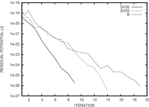
In the surface calculations obtaining the self-consistent one-electron potential is often a task of difficulty, because a large unit cell causes the electron density to slosh easily. Thus we have chosen (110) unrelaxed surfaces of silicon and gallium arsenide as the first two stringent test examples to show the properties of the SV prediction operator. A unit cell representing the (110) surface of each semiconductor contains ten atoms. The initial input one-electron potential is obtained from a linear superposition of electron density of the constituent atoms. When the SV prediction operator is employed, two special choices forNeigare chosen:Neig¼25

and Neig¼35. In each case all the calculated states have

participated in constructing the SV prediction operator. If the surface were insulating, we would need to deal with only the twenty lowest states. For comparison, the storage-saving, multiple-secant variant of Broyden’s algorithm alone is also employed.

For the Si surface, Fig. 1 shows on a semilogarithmic scale the iteration number versus an infinity norm of the residual potentialVres:

max

~ G G

jVresðGG~Þj:

The SV prediction operator has brought us the faster convergence. Increasing Neig leads to greater performance.

This is consistent with the fact that projecting the Hamil-tonian operator on a wider subspace (eq. (26)) is equivalent to imitating the Hamiltonian appeared in the left-hand side of the original KS secular equation (eq. (3)) more precisely.

For the GaAs surface, as shown in Fig. 2, the residual potential has converged slightly more slowly than for the Si surface. The overall results are, however, quite similar to those of the Si surface. Therefore, the SV prediction operator is highly recommendable when the unit cell is large.

3.3 Intermetallic compounds

We now turn out attention to the intermetallic compounds. The third example is Ce3Al in the L12 structure. Ce3Al exhibits high density of states near the Fermi energy originating in the4f and5d shells of the Ce atoms,2)which implies that a small change in the input one-electron potential

Vincauses a large change in the electron density, and thus in

the residual potential Vres. Therefore dealing with Ce3Al is another stringent test of the SV prediction operator. When the SV prediction operator is employed, two special choices for

Neigare chosen:Neig¼40andNeig¼50. Since5psemicore

[image:5.595.307.546.73.244.2]

states in the Ce atoms are treated explicitly in the present study, if Ce3Al were an insulator, the seventeen lowest states would suffice. In practice, however, typically the thirty-five lowest states are occupied significantly by valence and semicore electrons.

Figure 3 shows the convergence of the residual potential

Vres. Introducing the SV prediction operator has reduced the

1e-27 1e-26 1e-25 1e-24 1e-23 1e-22 1e-21 1e-20 1e-19 1e-18

2 4 6 8 10 12 14 16

RESIDUAL POTENTIAL (J)

ITERATION

SV35 SV25 B

Fig. 1 Convergence in the residual potentialVresin the case of the Si (110) surface. SVmdenotes the SV prediction operator constructed using them

lowest states at each iteration step, while B does the storage-saving, multiple-secant variant of Broyden’s algorithm. 1:0en stands for 1:010n_.

1e-27 1e-26 1e-25 1e-24 1e-23 1e-22 1e-21 1e-20 1e-19 1e-18

2 4 6 8 10 12 14 16 18 20

RESIDUAL POTENTIAL (J)

ITERATION

SV35 SV25 B

Fig. 2 Same as Fig. 1, except for the GaAs (110) surface.

1e-28 1e-27 1e-26 1e-25 1e-24 1e-23 1e-22 1e-21 1e-20 1e-19

2 4 6 8 10 12 14 16 18

RESIDUAL POTENTIAL (J)

ITERATION

SV50 SV40 B

[image:5.595.49.291.554.726.2] [image:5.595.312.548.592.768.2]

iterations more dramatically than in the case of the semi-conductor surfaces. Moreover, when the SV prediction operator is used, the convergence for Ce3Al is less heavily dependent onNeigthan for the semiconductor surfaces. This

indicates that the lowest and a few additional states, required to calculate the electron density properly, suffice to construct the efficient SV prediction operator for such metals as Ce3Al, which exhibits high density of states around the Fermi level. Ni3Al, in theL12 structure, is an intermetallic compound of theoretical magnetic moment per unit cell ranging from almost 0 to4:081024_J/T.65–68)_{This fluctuation suggests}

that Ni3Al lies near a threshold for the occurrence of the magnetic moment. In such a system the magnetic moment does not converge so smoothly or quickly as does the one-electron potential.48,69) Since the SV prediction operator incorporates the nonlinearity ofUU^ in eq. (9), however, it will make both the magnetic moment and the one-electron potential converge smoothly as well as quickly. This ex-pectation has led us to select the spin-polarized calculation of Ni3Al as the last test example. When the SV prediction operator is employed, two special choices forNeigare chosen: Neig¼30 and Neig¼35. If Ni3Al were an insulator, the seventeen lowest states would suffice. In practice, however, typically the nineteen lowest states are occupied significantly by valence electrons.

The SV prediction operator has accelerated the conver-gence inVin, as shown in Fig. 4, no matter how many states

are calculated. In addition, as shown in Fig. 5, the magnetic moment converges smoothly with the SV prediction oper-ator; otherwise it stalls until the tenth iteration step. Since our criterion of convergence is very tight, one may be tempted to loosen it. Comparison of Figs. 4 and 5, however, warns us that loosening the criterion to, for example, 11024_Ry leads to uncertainty in the magnetic moment of11025_J/ T without the SV prediction operator. With this respect, the SV prediction operator makes the spin-polarized calculations be not only faster, but also more reliable.

4. Conclusion

In the present paper we have developed the SV predictoion operator to reduces the number of iterations required to

obtain the self-consistent one-electron potential for the first-principles electronic-structure calculations within the plane-wave-based pseudopotential framework. We have derived the SV prediction operator by projecting the KS equation on the subspace spanned with eigenstates obtained from a one-electron potential for the previous iteration step. Furthermore we have shown that the SV prediction operator can be combinined with the Broyden-like algorithm.

We have verified that the SV prediction operator brought about the rapid convergence of the one-electron potential in the electronic-structure calculations of the semiconductor surfaces and intermetallic compounds. Another advantage of the SV prediction operator is that when the magnetic moment occurs, it converges as smoothly as does the one-electron potential. Considering these results and the ease of imple-mentation of the SV prediction operator, we strongly recommend it to those who use plane-wave-based methods. Moreover, we expect the SV prediction operator to retain its excellence in such formalisms as difference and finite-element methods, where the wavefucntions are expressed by an inevitably huge number of variables.

Acknowledgements

The authors wish to thank Prof. R. Yamamoto for stimulating discussions.

REFERENCES

1) W. Kohn and L. J. Sham: Phys. Rev.140(1965) A1133–A1138. 2) D. D. Koelling: Rep. Prog. Phys.44(1981) 139–212.

3) G. P. Srivastava and D. Weaire: Adv. Phys.36(1987) 463–517. 4) J. Ihm: Rep. Prog. Phys.51(1988) 105–142.

5) W. E. Pickett: Comput. Phys. Rep.9(1989) 115–197.

6) D. K. Remler and P. A. Madden: Mol. Phys.70(1990) 921–966. 7) M. C. Payne, M. P. Teter, D. C. Allan, T. A. Arias and J. D.

Joannopoulos: Rev. Mod. Phys.64(1992) 1045–1097. 8) T. Ito: J. Appl. Phys.77(1995) 4845–4886.

9) R. G. Parr and W. Yang:Density-Functional Theory of Atoms and Molecules, (Oxford Univ. Press, Oxford, 1989) 1–324.

10) R. Car and M. Parrinello: Phys. Rev. Lett.55(1985) 2471–2474. 11) M. C. Payne, J. D. Joannopoulos, D. C. Allan, M. P. Teter and D. H. 1e-27

1e-26 1e-25 1e-24 1e-23 1e-22 1e-21 1e-20 1e-19

2 4 6 8 10 12 14

RESIDUAL POTENTIAL (J)

ITERATION

SV35 SV30 B

Fig. 4 Same as Fig. 1, except for Ni3Al.

1e-29 1e-28 1e-27 1e-26 1e-25 1e-24

2 4 6 8 10 12 14

ERROR IN MAGNETIC MOMENT(J/T)

ITERATION

SV35 SV30 B

[image:6.595.306.547.71.243.2] [image:6.595.49.289.594.767.2]

Vanderbilt: Phys. Rev. Lett.56(1986) 2656–2656.

12) A. Williams and J. Soler: Bull. Am. Phys. Soc. B32(1987) 562–562. 13) I. Sˇtich, R. Car, M. Parrinrllo and S. Baroni: Phys. Rev. B39(1989)

4997–5004.

14) J. Garner, S. G. Das, B. I. Min, C. Woodward and R. Benedeck: Phys. Rev. B39(1989) 12899–12902.

15) G. W. Fernando, G.-X. Quian, M. Weinert and J. W. Davenport: Phys. Rev. B40(1989) 7985–7988.

16) M. P. Teter, M. C. Payne and D. C. Allan: Phys. Rev. B40(1989) 12255–12263.

17) M. J. Gillan: J. Phys. C1(1989) 689–711.

18) Y. Yamamoto and T. Fujiwara: Phys. Rev. B46(1992) 13596–13598. 19) F. Tassone, F. Mauri and R. Car: Phys. Rev. B50(1994) 10561–10573. 20) M. P. Grumbach, D. Hohl, R. M. Martin and R. Car: J. Phys. C.6

(1994) 1999–2014.

21) J. Hutter, H.P. Lu¨thi and M. Parrinello: Comput. Mater. Sci.2(1994) 244–248.

22) Y. Zempo, M. Ishida and M. Yoshida: J. Mol. Struct. (Theochem)310 (1994) 17–21.

23) M. Kohyama: Modelling Simul. Mater. Sci. Eng.4(1996) 397–408. 24) G. Kresse and J. Furthmu¨ller: Comput. Mater. Sci.6(1996) 15–50. 25) G. Kresse and J. Furthmu¨ller: Phys. Rev. B54(1996) 11169–11186. 26) J. L. Martins and M. L. Cohen: Phys. Rev. B37(1988) 6134–6138. 27) Since we certainly cannot list all the papers concerned with iterative

algorithms for the eigenvalue problem, we would like to introduce to the reader excellent bibliographies, A. Knyazev, http://liinwww.ira. uka.de/bibliography/Math/eigenproblem.html and http://liinwww. ira.uka.de/bibliography/Math/eigensolvers.html.

28) D. G. Anderson: J. Assoc. Comput. Mach.12(1965) 547–560. 29) C. G. Broyden: Math. Comput.19(1965) 577–593.

30) P. Pulay: Chem. Phys. Lett.73(1980) 393–398. 31) P. Pulay: J. Comput. Chem.3(1982) 556–560. 32) G. P. Kerker: Phys. Rev. B23(1981) 3082–3084.

33) K.-M. Ho, J. Ihm and J. D. Joannopoulos: Phys. Rev. B25(1982) 4260–4262.

34) B. I. Dunlap: Phys. Rev. A25(1982) 2847–2849.

35) P. Bendt and A. Zunger: Phys. Rev. B26(1982) 3114–3137. 36) G. P. Srivastava: J. Phys. A17(1984) L317–L321.

37) D. Vanderbilt and S. G. Louie: Phys. Rev. B30(1984) 6118–6130. 38) D. D. Johnson: Phys. Rev. B38(1988) 12807–12813.

39) J. F. Anett: Comput. Mater. Sci.4(1995) 23–42. 40) X. Gonze: Phys. Rev. B54(1996) 4383–4386. 41) V. Eyert: J. Comput. Phys.124(1996) 271–285.

42) M. Kawata, C. M. Cortis and R. A. Friesner: J. Chem. Phys.108(1998) 4426–4438.

43) A. Sawamura, M. Kohyama, T. Keishi and M. Kaji: Mater. Trans., JIM 40(1999) 1186–1192.

44) J. Auer and E. Krotscheck: Comput. Phys. Comm.118(1999) 139–144. 45) D. R. Bowler and M. J. Gillan: Chem. Phys. Lett.325(2000) 473–476. 46) A. Trellakis, A. T. Galick, A. Pacelli and U. Ravaioli: J. Appl. Phys.81

(1997) 7880–7884.

47) A. H. MacDonald, W. E. Pickett and D. D. Koelling: J. Phys. C13 (1980) 2675–2684.

48) D. J. Singh:Planewaves, Pseudopotentials and the LAPW Method, (Kluwer Academic Publishers, Boston, 1994) 1–115.

49) J. Ihm, A. Zunger and M. L. Cohen: J. Phys. C.12(1979) 4409–4422. 50) J. Ihm, A. Zunger and M. L. Cohen: J. Phys. C.13(1980) 3095–3095. 51) P. J. H. Denteneer and W. van Haeringen: J. Phys. C.18(1985) 4127–

4142.

52) D. M. Ceperly and B. J. Alder: Phys. Rev. Lett.45(1980) 566–569. 53) J. Perdew and A. Zunger: Phys. Rev. B23(1981) 5048–5079. 54) A. M. Rappe, K. M. Rabe, E. Kaxiras and J. D. Joannopoulos: Phys.

Rev. B41(1990) 1227–1230.

55) A. M. Rappe, K. M. Rabe, E. Kaxiras and J. D. Joannopoulos: Phys. Rev. B44(1991) 13175–13176.

56) N. Troullier and J. S. Martins: Phys. Rev. B43(1991) 1993–2006. 57) G. Kresse and J. Hafner: J. Phys. C6(1994) 8245–8257. 58) E. R. Davidson: J. Comput. Phys.17(1975) 87–94. 59) E. R. Davidson: Comput. Phys. Comm.53(1989) 49–60.

60) A. Sawamura, M. Kohyama and T. Keishi: Comput. Mater. Sci.14 (1999) 4–7.

61) L. Keinman and D. M. Bylander: Phys. Rev. Lett.48(1982) 1425– 1428.

62) P. E. Blo¨chl: Phys. Rev. B41(1990) 5414–5416. 63) M. Teter: Phys. Rev. B48(1993) 5031–5041.

64) S. G. Louie, S. Froyen and M. L. Cohen: Phys. Rev. B26(1982) 1738– 1742.

65) D. Hackenbracht and J. Ku¨bler: J. Phys. F10(1980) 427–440. 66) J. J. M. Buiting, J. Ku¨bler and F. M. Mueller: J. Phys. F13(1983)

L179–L184.

67) B. I. Min, A. J. Freeman and H. J. F. Jansen: Phys. Rev. B37(1988) 6757–6762.

68) J.-H. Xu, B. I. Min, A. J. Freeman and T. Oguchi: Phys. Rev. B41 (1990) 5010–5016.