Models and data analysis tools for the Solar Orbiter mission

Models and data analysis tools for the Solar Orbiter mission

A. P. Rouillard

, R. F. Pinto

, A. Vourlidas

, A. De Groof

, W. T. Thompson

, A. Bemporad

, S. Dolei

, M. Indurain

,

E. Buchlin

, C. Sasso

, D. Spadaro

, K. Dalmasse

, J. Hirzberger

, I. Zouganelis

, A. Strugarek

, A. S. Brun

, M.

Alexandre

, D. Berghmans

, N.E. Raouafi

, T. Wiegelmann

, P. Pagano

, C. N. Arge

, T. Nieves-Chinchilla

,

M. Lavarra

, N. Poirier

, T. Amari

, A. Aran

, V. Andretta

, E. Antonucci

, A. Anastasiadis

, F. Auchère

, L.

Bellot Rubio

, B. Nicula

, X. Bonnin

, M. Bouchemit

, E. Budnik

, S. Caminade

, B. Cecconi

, J. Carlyle

, I.

Cernuda

, J.M. Davila

, L. Etesi

, F. Espinosa Lara

, A. Fedorov

, S. Fineschi

, A. Fludra

, V. Génot

, M. K.

Georgoulis

, H. R. Gilbert

, A. Giunta

, R. Gomez-Herrero

, S. Guest

, M. Haberreiter

, D. Hassler

, C. J.

Henney

, R. A. Howard

, T. Horbury

, M. Janvier

, S. I. Jones

, K. Kozarev

, E. Kraaikamp

, A.

Kouloumvakos

, S. Krucker

, A. Lagg

, J. Linker

, B. Lavraud

, P. Louarn

, M. Maksimovic

, S. Maloney

, G.

Mann

, A. Masson

, D. Müller

, H. Önel

, P. Osuna

, D. Orozco Suarez

, C. J. Owen

, A. Papaioannou

, D.

Pérez-Suárez

, J. Rodriguez-Pacheco

, S. Parenti

, E. Pariat

, H. Peter

, S. Plunkett

, J. Pomoell

, J. M. Raines

,

T. L. Riethmüller

, N. Rich

, L. Rodriguez

, M. Romoli

, L. Sanchez

, S. K. Solanki

, O. C. St Cyr

, T.

Straus

, R. Susino

, L. Teriaca

, J. C. del Toro Iniesta

, R. Ventura

, C. Verbeeck

, N. Vilmer

, A. Warmuth

, A.

Walsh

, C. Watson

, D. Williams

, Y. Wu

, and A. N. Zhukov

(Affiliations can be found after the references)

Received February 19, 2019; accepted XX

ABSTRACT

Context.The Solar Orbiter spacecraft will be equipped with a wide range of remote-sensing (RS) and in-situ (IS) instruments to record novel and unprecedented measurements of the solar atmosphere and the inner heliosphere. To take full advantage of these new datasets, tools and techniques must be developed to ease multi-instrument and multi-spacecraft studies. In particular the currently inaccessible low solar corona below two solar radii can only be observed remotely. Furthermore techniques must be used to retrieve coronal plasma properties in time and in three dimensional (3D) space. Solar Orbiter will run complex observation campaigns that provide interesting opportunities to maximise the likelihood of linking IS data to their source region near the Sun. Several RS instruments can be directed to specific targets situated on the solar disk just days before data acquisition. To compare IS and RS, data we must improve our understanding of how heliospheric probes magnetically connect to the solar disk. Aims.The aim of the present paper is to briefly review how the current modelling of the Sun and its atmosphere can support Solar Orbiter science. We describe the results of a community-led effort by European Space Agency (ESA)’s Modelling and Data Analysis Working Group (MADAWG) to develop different models, tools, and techniques deemed necessary to test different theories for the physical processes that may occur in the solar plasma. The focus here is on the large scales and little is described with regards to kinetic processes. To exploit future IS and RS data fully, many techniques have been adapted to model the evolving 3D solar magneto-plasma from the solar interior to the solar wind. A particular focus in the paper is placed on techniques that can estimate how Solar Orbiter will connect magnetically through the complex coronal magnetic fields to various photospheric and coronal features in support of spacecraft operations and future scientific studies.

Methods.Recent missions such as STEREO, provided great opportunities for RS, IS, and multi-spacecraft studies. We summarise the achievements and highlight the challenges faced during these investigations, many of which motivated the Solar Orbiter mission. We present the new tools and techniques developed by the MADAWG to support the science operations and the analysis of the data from the many instruments on Solar Orbiter. Results.This article reviews current modelling and tool developments that ease the comparison of model results with RS and IS data made available by current and upcoming missions. It also describes the modelling strategy to support the science operations and subsequent exploitation of Solar Orbiter data in order to maximise the scientific output of the mission.

Conclusions.The on-going community effort presented in this paper has provided new models and tools necessary to support mission operations as well as the science exploitation of the Solar Orbiter data. The tools and techniques will no doubt evolve significantly as we refine our procedure and methodology during the first year of operations of this highly promising mission.

Key words. Sun: Solar wind, numerical modeling, solar corona, coronal mass ejections, energetic particles

1. General introduction:

Heliophysics is at the dawn of a golden age in observational capabilities. In addition to the on-going space missions like ? _{Corresponding author: Alexis P. Rouillard e-mail:}

[email protected]

the Solar-TErrestrial RElations Observatory (STEREO, Kaiser et al. 2008), the SOlar and Heliophysics Observatory (SOHO, Domingo et al. 1995), the Solar Dynamics Observatory (SDO, Pesnell et al. 2012), Hinode (Hinode, Tsuneta et al. 2008b), and the Interface Region Imaging Spectrograph (IRIS, De Pontieu et al. 2014), space agencies are launching in addition to Solar Orbiter (Solar Orbiter) (Müller et al. 2019), described in detail here, the following two complementary missions: the Parker Solar Probe by NASA and PROBA-3 by ESA. Parker Solar

Probe (PSP, Fox et al. 2016), which was launched on 12 August 2018, will, for the first time, measure the properties of the solar corona as close as nine solar radii from the solar surface. The PROBA-3 (Lamy et al. 2010; Renotte et al. 2016) will provide unprecedented white-light imaging of the low corona thanks to its revolutionary spacecraft (S/C) formation flying which reproduces the ideal observing conditions of solar eclipses. Data acquisition from the ground-based observatories such as the Global Oscillation Network Group (GONG, Hill et al. 1994; Harvey et al. 1996), GREGOR (GREGOR, Schmidt et al. 2012), and the Swedish 1-m Solar Telescope (SST, Scharmer et al. 2003); ground-based radio telescopes and neutron monitors spread around the globe; the Low-Frequency Array (LOFAR, van Haarlem et al. 2013) and the Daniel K. Inouye Solar Telescope (DKIST, Keil et al. 2011; Warner et al. 2018) will provide crucial complementary data. To take full advantage of this data so that we maximise our chances of answering the fun-damental questions on the solar atmosphere, we need advanced data-analysis techniques and models capable of exploiting the multi-instrumental and multi-viewpoint data obtained by these observatories. The Modeling and Data Analysis Working Group (MADAWG) was created by ESA, in conjunction with two other working groups focused on the coordination of in-situ (IS) measurements (Horbury et al. 2019b) and remote-sensing (RS) observations (Auchere et al. 2019)) to address these challenges head on, adapt existing tools and develop new ones to prepare scientific studies with Solar Orbiter and the future heliophysics observatories.

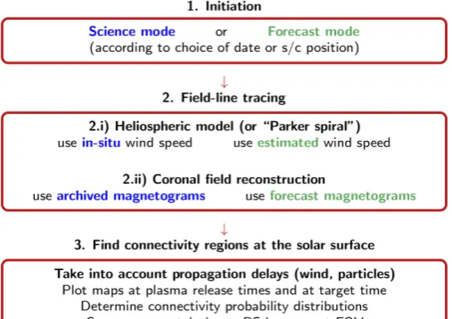
A majority of Solar Orbiter science goals rely on coor-dinated observations with multiple instruments (Müller et al. 2019), from IS instruments (Maksimovic et al. 2019; Horbury et al. 2019a; Owen & et al. 2019; Rodríguez-Pacheco et al. 2019) operating continuously along the orbit beginning in cruise phase, to the RS instruments (SPICE Consortium et al. 2019; Solanki et al. 2019; Krucker et al. 2019; Antonucci et al. 2019; Rochus et al. 2019; Howard et al. 2019) observing during three 10-day windows per orbit called Remote Sensing Windows (RSWs). The RSWs will typically be centred around perihelia as well as minimum and maximum heliographic latitudes. The operational constraints including limited telemetry due to orbital characteristics, variable data latency (up to 180 days) due to large variations in S/C-Earth distance, and limited memory space on board motivated the need for long-term planning of top-level science operations (Zouganelis et al. 2019). The mission science outcome depends on coordinated observations of unpredictable solar activity. The high-resolution science requires fine-pointing to a target which position cannot be pre-planned. Moreover the nominal period of operation of Solar Orbiter is about seven years, hence covering more than half a solar activity cycle from solar minimum to maximum, the latter being currently expected to occur around 2024. This means that we can expect large variations of the activity level of the Sun during the nominal phase.

The science planning (Zouganelis et al. 2019) therefore folds in several time frames for mission level planning that depend on coordinated observations during opportunity windows along the trajectory, variable down link and limited memory on board as well as restrictions on RS observation time, telemetry man-agement, and incompatibilities in electromagnetic cleanliness (EMC). The long-term plan (T - 12 to 6 months), medium-term plan (T - 1 month), short-term plan (T - 1 week) and very short term planning (VSTP) of science operations are described in the

science planning article in the present volume (Zouganelis et al. 2019). During the latter VSTP, the high-resolution FOVs, that is PHI’s High-Resolution Telescope (PHI/HRT, Solanki et al. 2019), the EUI High-resolution Imagers (EUI/HRI, Solanki et al. 2019) and the spectrometer SPICE (SPICE Consortium et al. 2019), require fine-pointing to target while changing solar activity will impose pointing updates with short turn-around for data selection and calibration updates. To provide the necessary visibility, low-latency (i.e. quicklook) data will be required (Sanchez et al. 2019).

Low-latency data, combined with modeling, can provide an important role for forecasting the location of targets and their magnetic connection with the S/C to choose targets and update the pointing. Once data has been acquired, models and tools will help interpret the daily low-latency data and decide which on-board data to select or prioritise for downlink (for those instruments with internal-storage, or those IS instruments using selective downlink capabilities). This is an important step to increase the likelihood of scientific studies that require combined IS-RS datasets. We described in this article the tools and models that we have put into place to help within this complex operational context.

Modeling also plays a central role for data analysis once the final data has been transmitted to the ground for the many reasons that are addressed in this article. Modeling compensates for an inherently incomplete sensing of the solar corona, can help connect different datasets and overall has become an essential tool to evaluate theories. At the time of writing this article we have not yet measured plasma IS in the corona inside 10 solar radii, solar plasma has been measured IS as close as 0.3 AU and as far as the limits of the heliosphere. Yet the physical mechanisms that produce the heating of the corona, the formation of the solar wind, the acceleration of solar energetic particles and Coronal Mass Ejections (CMEs) operate in the solar corona well inside 10 solar radii. To test the various theories and models proposed to exploit these phenomena, we need to retrieve the time-dependent evolution of the coronal plasma properties using different techniques supported by numerical models.

field structure of the corona is also very incomplete since we measure the full 3D magnetic field only in certain regions of the photosphere and chromosphere. Reconstruction techniques and models must be used to retrieve the 4D structure of the quiet and transient corona (see section 4), this is absolutely essential to make any kind of progress in our understanding of fundamental coronal processes. When connection can be established between particles and fields measured IS with their sources at the Sun, then a more complete picture of the physical processes coupling the solar corona to the heliosphere can be established (see section 5). All these constitute the great challenges that we face to prepare the Solar Orbiter mission.

2. Heritage of the recent STEREO era

The Sun-Earth Connection Coronal and Heliospheric

Investi-gation (SECCHI; Howard et al. 2008) onboard the STEREO

mission has provided since 2007, unprecedented imaging of solar storms from vantage points situated outside the Sun-Earth line. STEREO offered for the first time an uninterrupted imaging of plasma flows from the Sun to the Earth-like distances. The analysis of wide-angle imaging from multiple vantage points motivated the development of many algorithms and software tools in the last 10-15 years. The tools primarily focus on deriv-ing the 3D morphology of coronal and heliospheric structures, estimating their kinematics and direction of propagation in the corona and heliosphere. The following sections are purely intended to illustrate the power of using multiple viewpoints to infer the properties of coronal structures such as background streamers, coronal holes, CME flux ropes, shock waves. These techniques are being adapted and improved in preparation for Solar Orbiter as they have become integral parts of IS-RS studies (see section 3).

2.1. Locating coronal and solar wind structures in 3D

To locate structures in the optically-thin corona, 3D reconstruc-tions techniques constrained directly by coronal observareconstruc-tions have been made freely available in the IDLSolarsoftdistribution package, they include the basic Potential Field Source Surface (PFSS) model (e.g. Schrijver & De Rosa 2003), software for 3D reconstructions of coronal loops (e.g., Aschwanden et al. 2009), flux ropes (e.g. Thernisien et al. 2009), and shocks (e.g. Vourl-idas & Ontiveros 2009; Kwon et al. 2014). These techniques deploy forward modeling approaches, where the user attempts to fit a geometric shape, such as an ellipsoid for a shock or a ’croissant’-like structure for a flux rope, on snapshots of the tran-sient in two or three simultaneous views.

The requirement of fitting the forward model in multiple views simultaneously tightly constraints the fit and results in quite ro-bust reconstructions. To minimise the amount of free parameters, most models are rooted at Sun centre, rather than the source re-gion (hence deflections are harder to simulate) and ignore small scale distortions on the modelled shape (hence local distortions of the structure are not modelled). Such models are generally better suited for examining the evolution of the large-scale en-velope of transients and for investigating rotations or depar-tures from self-similar expansion. More complex forward mod-els have been used to account for distorted or irregular shapes of flux ropes and shocks (Wood et al. 2009) and for reconstruct-ing (and locatreconstruct-ing the solar origin) of Corotatreconstruct-ing Interaction Re-gions CIRs (Wood et al. 2010) that were first identified in

he-liospheric images by Rouillard et al. (2008) and Sheeley et al. (2008). A simpler approach to 3D reconstruction is the localiza-tion in space of a single point in a structure via direct geometric triangulation, also referred to as tie-pointing. The accuracy of the technique relies on the ability to identify the same feature in images from two viewpoints, preferably taken at the same time. This is not always an easy task, either in the low corona, where features are small and can be obscured by the viewing geometry, or the outer corona, where the features are generally smoother and much more extended in space. An example and the issues behind tie-pointing in the outer corona are discussed in Liewer et al. (2011). The techniques work well for features with intrin-sic small-scale structure, such as prominences (e.g., Panasenco et al. 2013; Thompson 2013) and comet tails (e.g., Thompson 2009). The tie-pointing routines are compatible with all WCS-compliant FITS data and are available inSolarsoft.

2.2. Feature tracking and trajectory analysis

Other techniques are used to derive 3D trajectories and the kinematic properties of out-flowing features in the outer corona and inner heliosphere from height-time measurements of a fea-ture. The techniques differ in their geometric assumption for transforming the observed elongation of the front (or other fea-ture) to heliocentric distance. The most popular assumptions are: the point propagates radially (fixed-φapproximation; Kahler & Webb 2007); the point lies at the Thomson Surface (point-P approximation); the point lies on the surface of an expanding sphere centered on the Sun (Harmonic Mean approximation; Lugaz et al. 2009); the point lies on the surface of a self-similarly expanding sphere propagating radially away from the Sun (Self-Similar Expansion approximation; Davies et al. 2013). Obvi-ously, all of these approximations make rather strong assump-tions about the direction and shape of the feature in question. The resulting kinematics should be interpreted carefully, as discussed in the comparison study by Lugaz (2010), which suggest that the radial propagation appears to be the more robust approximation. However, these approaches have some advantages. The fixed-phi technique is thought to be most adequate to determine the trajec-tory of streamer blobs far out in the heliospheric and connect those with IS measurements (Rouillard et al. 2010a,b). They are easy and quick to calculate and can be applied to single view-point measurements (preferably from offthe Sun-Earth line). A comprehensive application and comparison of these techniques in deriving the kinematic properties of CMEs in the inner helio-sphere is given in Möstl et al. (2014). All these techniques have been integrated in J-map visualization tools available either in Solarsoftsuch as SATPLOT (see section 6.5.1) or via interactive web-based interfaces such as the Propagation Tool (see section 6.5.2: Rouillard et al. 2017)

Fig. 1.A figure illustrating a successful linkage between a CME ob-served in white-light on STEREO-A on 3 June 2008 (panel e) with sub-sequent in situ signature at STEREO-B on 7 June 2008: the top pan-els show (a) plasma beta, (b) total plasma pressure, (c) number density from 2 to 7 June 2008 measured at B. (middle) STEREO-A elongation-time J-map combining HI-1 and HI-2 running difference images. The vertical dotted lines mark the extent of the ICME (Inter-planetary Coronal Mass Ejection) signature in the STEREO-B data. The ICME boundaries closely match the region bounded by the leading and trailing elongation-time tracks in the STEREO-A data (black arrows). The bottom panel displays one of the HI-1A running-difference images employed to build the J-map. From Rouillard (2011). Reprinted by per-mission of Solar Physics.

elongation as a function of time. Their kinematics can be eas-ily derived by fitting a variety of curves on these tracks based on the techniques introduced in the previous section. Crossing of tracks readily identify CME-CME or CME-CIR interactions. Diverging tracks in the low corona can mark the locations of collapsing loops such as those observed in the source regions of streamer blobs (e.g., Sanchez-Diaz et al. 2017a,b; Wang & Hess 2018). Diverging tracks can also result from projection effects associated with radially out-flowing transients emitted by a sin-gle source region co-rotating away from the observer, these were recurrently observed in HI images taken by STEREO-B (e.g., Rouillard et al. 2010a). J-maps can also be used to connect, in a concise way, solar structures to their IS counterparts as illus-trated in Fig. 1 (see review by Rouillard (2011) for more exam-ples). Overall J-maps are extremely useful but must be analysed with care due to projection effects.

2.3. Challenges faced so far when relating RS with IS data:

We illustrate briefly three areas where good progress has been achieved in recent years by combining RS and IS using recon-struction and tracking techniques such as those described in the previous paragraph. This will motivate the next parts that present recent and upcoming developments to improve models and tools for Solar Orbiter science.

2.3.1. Linking CMEs with ICMEs

Magnetometers onboard heliospheric observatories in the near-Earth environment sometimes display clear signatures of helical magnetic fields. A subset of those are called magnetic clouds (Burlaga et al. 1981) when a smooth and large magnetic field rotation is observed with associated drops in plasma beta and temperature. This helical topology is likely intimately linked to the initiation process of CMEs (e.g., Gosling 1990; Gopalswamy et al. 1998). RS detectors such as the coronagraphs and helio-spheric imagers onboard STEREO or SOHO display change in the coronal structure with the appearance of bright features in white-light observations (e.g., Vourlidas & Howard 2006; Webb et al. 2012). The observed patterns in the brightness of RS ob-servations are studied as different CME components (Vourlidas et al. 2013). The core, usually observed remotely as a dark area is surrounded by a bright rim and is accepted to be the flux rope cavity. The IS signature of this cavity long suspected to be the magnetic cloud (Dere et al. 1999; Wood et al. 1999), was clearly identified as such using STEREO J-maps by Möstl et al. (2009) and Rouillard et al. (2009). The brightness in the front defines the leading edge associated with the sheath and interplanetary (IP) shock in the in situ observations (e.g., Kilpua et al. 2011).

Lynch et al. (2010) and the review by Rouillard (2011) (see Fig. 1) paint a rather positive picture for our ability to con-nect RS observations and IS measurements of certain interplan-etary propagating (IP) structures, particularly under solar min-imum conditions. The reality, however, is more complicated. Despite the availability of continuous imaging and tracking of IP disturbances from the STEREO heliospheric imagers, CME time-of-arrivals and especially speeds at 1 AU can have errors upwards of 13 h and 200 km s−1_{, respectively, even for}

et al. 2011; Nieves-Chinchilla et al. 2013b). In contrast, from the in situ perspective, the magnetic field strength asymmetries observed can be interpreted as a consequence of the local ef-fect of flux rope expansion (Farrugia et al. 1993; Osherovich et al. 1993; Démoulin & Dasso 2009) or erosion (Dasso et al. 2007; Ruffenach et al. 2012), but it could also be a result of the distortion (Hidalgo et al. 2002; Berdichevsky 2013; Nieves-Chinchilla et al. 2018b). Longitudinal deflections during inner heliospheric transit are particularly hard to quantify because he-liospheric imaging is taken from and restricted along the eclip-tic plane. This is the reason, for example, why the “garden-hose spiral” nature of solar wind streams has never been imaged di-rectly but only inferred by de-projection techniques based on J-maps (Rouillard et al. 2008; Sheeley et al. 2008). While major progress was achieved with STEREO data, establishing the ex-act longitudinal extent of streamer blowouts (Vourlidas & Webb 2018), whether CMEs deflect longitudinally or merge with each other, where CIRs form or how shocks evolve require observa-tions away from the ecliptic (Gibson et al. 2018). This is an area where Solar Orbiter imaging, particularly from Solar OrbiterHI (Howard et al. 2019) will be trailblazing. However to fully ex-ploit this data we need to adapt our techniques to account for rapidly varying vantage points located outside the ecliptic plane.

2.3.2. Linking particle accelerators with SEPs

The onset of large CMEs can suddenly transform the corona into an efficient particle accelerator. Solar Energetic Particle (SEP) events can be produced by CME-driven shocks or by other acceleration processes in association with flares. The many processes that can produce SEP events are not well understood and more importantly not very well distinguishable from particle measurements made at 1 AU. The link between solar storms (CMEs and flares), the perturbations of the corona they induce and the production of Solar Energetic Particles is a topic of active research. We briefly illustrate recent results that exploited RS-IS observations from multiple vantage points to investigate the link between CME substructures and SEPs. We highlight the challenges faced that have motivated the developments of new models and techniques for Solar Orbiter.

HELIOS measurements near 0.3 AU have revealed that a seemingly single gradual SEP event measured near 1 AU can appear more complex at 0.3 AU with the occurrence of multiple peaks in SEP fluxes suggesting that multiple events occurred successively. These multiple flux enhancements are presumably due to the changing conditions at the particle source that is magnetically connected to the S/C but the propagation effects merge the events into one single long-lasting flux enhancement and decrease by 1 AU. This can either result from a changing magnetic connection to different particle accelerators or else from a single accelerator with strongly varying properties. It is therefore crucial to make measurements of energetic particles closer to the acceleration site so as to disentangle the properties linked to the acceleration site from the effects of particle transport.

The outer boundary of CMEs imaged in coronagraphs is the most likely location for shocks to develop as they mark the transition between the transient and the background corona. This region has therefore been the focus of many studies exploiting SOHO and STEREO data. The challenge resides in inferring when and where a shocks form on this bound-ary. Some early techniques derived, from a single viewpoint

situated along the Sun-Earth line (SOHO), the properties of shocks driven by CMEs propagating in the plane of the sky (Bemporad & Mancuso 2013). Improvements were brought by the application of 3D shock reconstruction techniques (see 2.1) to STEREO images from multiple viewpoints (e.g., Kwon et al. 2014; Rouillard et al. 2016). Important information on the formation and evolution of shock waves in the solar corona could then be obtained. Processing of these reconstructions provided the de-projected 3D expansion speed of the moving fronts in the corona for most CME directions (e.g., Rouillard et al. 2016), those speeds can be compared to the ambient Alfvén and magnetosonic speeds of the corona (provided by 3D models of the background solar corona) to derive the 3D Mach number of the entire moving shock. Recent studies have shown that pressure waves become shocks early on during the CME event (e.g., Rouillard et al. 2016; Plotnikov et al. 2017).

In order to compare derived shock properties with SEPs we need to determine how the shock connects magnetically to the S/C making in-situ measurements. This is likely the hardest and most uncertain step because, as already stated before, our knowl-edge of 3D magnetic fields both in the corona and in the inner heliosphere is uncertain. This point motivates the discussion in section 5. The simplest approach typically used is to consider that the interplanetary magnetic field extending between a S/C measuring SEPs and the upper corona is an Archimedean spi-ral defined by the plasma speed measured IS during the SEP. This spiral is traced down from the upper corona (typically at a source surface situated at 2.5 Rs) to the photosphere using a coronal model (see section 4.1.1). The alternative is to use the results of full magnetohydrodynamic (MHD) models typi-cally made available by numerical modellers via the Commu-nity Coordinated Modelling Center (CCMC, https://ccmc. gsfc.nasa.gov/). Comparative studies between shock waves and SEPs suggest a link between the strength of the shock quan-tified by the Mach number and the scattering-center compression ratio and the intensity of the SEP measured IS (e.g., Rouillard et al. 2016; Kouloumvakos et al. 2019). However to validate the shock hypothesis many questions must still be resolved concern-ing the timconcern-ing, longitudinal spread and composition of SEPs and the relative role of shock waves and flares as particle accelerators (e.g., Lario et al. 2017). General conclusions from these recent studies highlight the importance of improving our knowledge of 3D plasma coronal parameters where the strongest particle ac-celeration is occurring and the absolute necessity to improve in our understanding of magnetic field connectivity between IS S/C and the low solar corona.

2.3.3. Linking coronal plasma to the solar wind properties

Detection of the heated coronal plasma by IS measurements is mediated by the outflowing solar wind. Research over the last two decades (e.g., Hansteen & Leer 1995; Cranmer et al. 1999; Lionello et al. 2009; Downs et al. 2010; van der Holst et al. 2014; Pinto & Rouillard 2017; Usmanov et al. 2018) has shown that realistic coronal densities and solar wind mass fluxes can only be achieved with a detailed treatment of the thermodynamic processes throughout the computational domain from the upper chromosphere to the inner heliosphere. Thermal conduction is extremely important to transfer energy from the hot corona to the chromosphere that in turn enhances radiative processes (with its cooling effects) as well as chromospheric evaporation (and associated mass flows) feeding the solar wind. These energy exchange mechanisms are intimately linked to the distribution of plasma properties in the upper chromosphere and low corona. Knowledge of plasma densities and temperatures in these regions is therefore essential and in order to compare RS observations with model one must use realistic computations of the global magnetic field topology. Forward-modelling techniques can then be applied to confront model results to WL (white Light) or EUV imaging and spectroscopic observations from the top of the chromosphere to the corona to test if the temperatures and densities are correctly reproduced by the model (e.g., Downs et al. 2010; van der Holst et al. 2014; Pinto & Rouillard 2017). Assuming that heavy ions have the same temperature as the main plasma constituents and some typical coronal abundances, the brightness of the corona in EUV predicted by 3D models can be compared with EUV images from STEREO and SDO. Techniques that exploit images and spectroscopy have also been put in place to infer the distribution of coronal plasma temperature and speed (see section 4.3) (e.g., Dolei et al. 2018) that can also be compared with coronal mod-els. In this respect, white-light images are crucial to determine if the position and brightness of streamers and pseudo-streamers are correctly reproduced. Synchronous maps produced from several vantage points have become essential tools to help with these model evaluations as described in section 4.2.

One step further is to consider the ionisation level of heavy ions. In recent studies RS and IS data have also been com-bined with numerical models to test solar wind models at heights where the ionisation level of heavy ions becomes frozen in (e.g., Landi et al. 2014). These studies compared the predicted coro-nal brightness of emission lines from carbon and oxygen ions derived from the output of different solar wind models (e.g., van der Holst et al. 2014; Cranmer et al. 1999) with spectro-scopic observations. The predicted charge-state ratios were also compared with IS measurements. So far coronal models tend to under-estimate both the intensity of different emission lines and the charge state of different ions (Oran et al. 2015). This points to an inadequate modelling of ionisation processes such as the ef-fect of non-thermal particles or the effect of differential particle flows. New global coronal models are currently being developed (including in the MADAWG) that fully couple the main and mi-nor constituents and incorporate non thermal particles as well.

3. Future opportunities to link Solar Orbiter RS with IS data to address some of the key science questions

We briefly highlight here some examples of great opportunities that Solar Orbiter data will bring for future studies combining IS and RS data. This part introduces some of the technical

chal-lenges that we are currently facing to prepare for the arrival of these new datasets. The sections that follow present the solutions that the MADAWG is proposing to address some of these chal-lenges.

3.1. Investigations on the corona and the origin(s) of the solar wind(s)

As introduced in the previous section, the chromosphere-corona and solar wind are a coupled system that must be modelled as such. In order to compare these global models with RS obser-vations forward modelling has become a powerful approach. A forward modeling technique computes from a 3D data cube of plasma properties (derived by a model) a synthetic image or spectra for a vantage point by accounting for emission, ab-sorption and scattering processes of electromagnetic radiation as self-consistently as possible. Forward modeling is an essen-tial step at evaluating 3D coronal models close to the Sun in regions that even PSP will not measure directly. Coronal models can today be constructed using observed magnetograms (from MDI, HMI, and soon from the PHI instrument of Solar Orbiter, see section 4.1.2) to produce a realistic distribution of open and closed field regions (Miki´c et al. 2018; Réville & Brun 2017). The FORWARD modeling package is the most complete pack-age available in SolarSoft (Gibson et al. 2016). This tool pro-duces images in most EUV and WL lines that will be obtained by Solar Orbiter and will have to be adapted to include the Solar Orbiter’s fields of views. FORWARD has also become a central tool to compute synthetic spectro-polarimetric images compara-ble with current (CoMP) and future (DKIST) ground-based in-strumentation. In addition, the CHIANTI database (Landi et al. 2013) can be used to produce synthetic brightness profiles in dif-ferent emission lines typically observed in the chromosphere and corona in the X, UV and visible ranges. Creating synthetic pro-files out of such models using CHIANTI or FORWARD, spectra and images will be compared to Solar Orbiter’s unique RS data. Solar Orbiter’s EUI, Metis and Solar OrbiterHI will give us a new viewpoint to test background coronal models using forward modelling or image inversion (section 4.3). Synthetic RS obser-vations from the polar regions will be very useful at checking the relative locations of streamers and coronal holes against EUI and Metis images. We will finally understand how open and closed field lines interact due to their concomitant rigid and differential rotations.

de-tailed investigations of the composition of the coronal and solar wind plasmas. This includes investigations on the anomalously high abundance of elements with low First Ionisation Potential (the so-called FIP effect,e.g. Pottasch 1964; Fludra & Schmelz 1999).

Solar Orbiter’s SPICE instrument will produce maps of the rel-ative abundance of heavy ions near the Sun that will be com-parable with measurements by HIS, and will allow the testing of the solar wind models (Fludra & Landi 2018). Comparison of charge states between HIS and SPICE will also be possible, though it will require additional information from a coronal elec-tron temperature model, since SPICE measurements occur at al-titudes below the freeze-in of charge states measured by HIS. Several charge state and elemental abundance ratios will be in-cluded in HIS low-latency data to facilitate these comparisons on the VSTP scale for science operations.

3.2. Investigations on the global structure and origin(s) of CMEs

Multiview and multipoint observations of the CME/ICMEs have established the basic framework for the understanding of the multitude of physical evolutionary processes that the CME un-dergoes in the interplanetary medium (see Manchester et al. 2017). The advent of STEREO has meant to be a driver for many studies but also uncovered many issues and discrepancies related with the initial CME stages and evolution throughout the inter-planetary medium.

The techniques described in section 2.2 are necessary when the RS observations are obtained from within the ecliptic plane and provide only direct information on the radial and latitudinal extent of out-flowing structures such as CMEs or CIRs. The EUI, Metis and Solar OrbiterHI instruments will acquire coronal and heliospheric images from outside the ecliptic plane and therefore provide for the first time a direct view of the longitudinal and radial extent of solar features. Combined with images taken from inside the ecliptic plane by STEREO, SOHO or PROBA-3 and PSP, the full 3D structure of CMEs, their flux ropes and shocks, will be derived with greater confidence. Currently, the debate about the CME global 3D morphology, magnetic field configuration, and implications in terms of heliospheric evolutionary physical processes is open. For instance, we currently have very little information on the structure of CME legs and how they slowly become part of the recently opened and closed solar magnetic flux. A polar view will provide valuable information on this transition especially combined with data from PSP much closer to the Sun.

3D reconstruction techniques developed for STEREO Thernisien et al. (2009); Isavnin (2016); Wood et al. (2017) are being adapted to include Solar Orbiter’s fields of view and since the observation campaigns are rather short we should be able to produce catalogues of these 3D reconstructions to support research by the community. An illustration of future opportunities to reconstruct coronal shock waves using Solar Orbiter, STEREO, PSP and near-Earth orbiting S/C is shown in Figure 2.

Following the path of current ICME catalogs from Wind, ACE or STEREO, Solar Orbiter suite of in-situ instruments will be a valuable resource to identify ICMEs along the wide range of Sun distances of the mission. By using the models and techniques described by Nieves-Chinchilla et al. (2016, 2018a), the 3D reconstructions of the flux ropes inside ICMEs

will be available for the community. Thus, for instance, this is a valuable resource to accomplish campaign event analysis when Solar Orbiter is at suitable conjunction with PSP, STEREO and/or near-Earth solar-heliospheric observatories (Wind, Advanced Composition Explorer, SOHO, DSCVR). The 3D in-situ reconstructions are the more direct way to evaluate how the CMEs contribute to solar magnetic flux and helicity balance.

Trajectory analysis techniques require some deeper modifi-cations. Indeed the slow motion of the STEREO S/C meant that a CME moving outwards outside the ecliptic plane remained at fairly constant position angle throughout its transient to 1 AU. This is no longer the case with Solar Orbiter or PSP and new techniques are currently being considered that rely heavily on forward modelling, integrating self-consistently the changing viewpoint of the probes and the scattering/emission processes. Estimated trajectories will allow us to test full MHD propaga-tion models as such as the EUHFORIA model (see Pomoell & Poedts 2018 and section 5.3). They will allow us to refine our un-derstanding as well as our predictive skills of propagating CMEs, especially during the crucial first phases of evolution after their onset.

3.3. Investigations on the properties and origin(s) of SEPs

The variability of SEPs suggests rapid changes in the properties of the accelerator and the magnetic connectivity of that acceler-ator to the point of IS measurements. To test further the shock acceleration scenario we must pursue modelling of the the evo-lution of shock waves as accurately as possible to enable a com-plete modelling of particle acceleration with realistic shock pa-rameters Afanasiev et al. (2018). Since the number of fast CME events that Solar Orbiter will observe during RSWs will be rather limited, catalogs of triangulated CME shock waves that integrate Solar Orbiter data will also be produced and made available to the community. In addition the proximity of Solar Orbiter to the corona means that standard techniques to derive the release time of SEPs measured by Solar Orbiter such as velocity dispersion analysis and spectra of the different SEP events may be more accurate than those produced near 1 AU and can also be made available to the community.

Better coronal models will improve our computations of shock properties and provide more reliable estimates of the magnetic connectivity between the shock and the energetic particle detectors Rodríguez-Pacheco et al. (2019). To this end, the 3D shock triangulation codes (e.g., Kwon et al. 2014) readily available inSolarSoftand the Coronal Analysis of SHocks and Waves (CASHeW) framework (Kozarev et al. 2017), compatible with SolarSoft routines will be modified to naturally include these new viewpoints. Remote observations from Solar Orbiter will also enable a more accurate geometrical characterization of coronal and interplanetary shocks, so that non-radial propa-gation and small-scale structure of the fronts may be accounted for. Current efforts to prepare for Solar Orbiter data exploitation include the coupling of particle acceleration based on the theory of diffusive-shock acceleration and shock-drift acceleration to the 3D shock modeling (Afanasiev et al. 2018, e.g.).

Orbiter3Dpos1.png

Solar Orbiter_3Dpos_1.png

Fig. 2.A schematic to illustrate the possible synergies between mis-sions located in the inner heliosphere on 30 September 2024. The figure shows the relative positions of the planets as well as the Sun, SOHO, Solar Orbiter, PSP and STEREO-A. The fields of view of a subset of the instruments onboard these missions is also shown (SOHO: C2/C3, STEREO: COR-1 and COR-2, Solar Orbiter: Metis). In addition the 3D structure typically used to fit a flux rope and a shock in 3D are also shown.

by STIX (Krucker et al. 2019) and EUI (Rochus et al. 2019). The detection of flare accelerated particles close to the Sun will significantly reduce the influence of particle transport on esti-mates of the particle travel time and then on the particle escape time. The in-situ detection with EPD of energetic electrons with temporally correlated radio type III observations with RPW (Maksimovic et al. 2019) and ground-based observatories (in the case when they observe the same portion of the solar disk), and hard X-ray flare observations with STIX will allow the electron solar source region to be located without ambiguity and the magnetic connectivity to the S/C be well established. A more precise timing and association between IS energetic electrons and X-ray emitting electrons will allow in particular to re-investigate the relationship between the in-situ electron spectra and the electron spectra at the sun deduced from X -ray observations (see (e.g., Krucker et al. 2007). In this respect, new models have been developed in recent years that couple the large-scale evolution of magnetic fields with the acceleration of particles and the injection of these particles into the open magnetic field (Snow et al. 2017).

3.4. Investigations on the origin of the solar magnetic field

The solar magnetism originates from dynamo action in the so-lar interior within and at the base of its convective envelope. The most realistic solar dynamo models today compute self-consistently the complex and nonlinear interplay between con-vection and magnetic field. They generally rely on a combi-nation of physical mechanisms such as: strong shear in the tachocline and throughout the convective envelope (the Omega

effect), vortical inductive turbulent motions (the alpha effect), advection of the magnetic flux by the meridional circulation, and emergence of magnetic structures through the photosphere (the Babcock-Leighton effect). Observations of the photospheric magnetic field of the Sun are extremely valuable for our under-standing of the internal processes sustaining the solar magnetic field, along with helioseismic constraints. In particular, the de-tailed knowledge of the magnetic properties of the Sun at high latitudes (magnetic flux transport, strength of the polar field) is of paramount importance because they will allow to better char-acterise the intricate process of global polar field reversal.

Solar Orbiter, and in particular the PHI instrument will shed new lights on these processes. Observations of the Zeeman effect at the pole will provide valuable insights on how the flux can-cels out when the solar magnetic field reverses, what is the rel-ative importance of the small scale magnetic flux near the pole (Tsuneta et al. 2008a; Shiota et al. 2012), and how ultimately the poloidal field is regenerated (Benevolenskaya 2004). Further-more, new constraints on the patterns of the differential rotation and meridional circulation at the pole will be obtained through correlation tracking of small features, direct imaging of Doppler shifts and helioseismic observations from a high latitude van-tage point. This will provide critical inputs for dynamo models that are generally sensitive to the flows and their structure at high latitude (Charbonneau 2010). The deeper structure of the flows sustaining the solar dynamo down to the solar tachocline will also be probed with more accuracy thanks to stereoscopic he-lioseismic observations combining Solar Orbiter and, e.g. SDO and GONG. Altogether more precise constraints on the flows and field of the Sun will help disentangle whether separate dynamo processes are acting in our star, by leveraging these new key observations from Solar Orbiter in 2D and 3D mean-field (e.g. Charbonneau 2010; Yeates & Muñoz-Jaramillo 2013; Karak & Miesch 2017), 3D turbulent small-scale (e.g. Vögler & Schüssler 2007), and 3D large-scale (e.g. Brun et al. 2015; Strugarek et al. 2018) models of the solar dynamo. An example of such mod-els can be found in Figure 3 where a solar-like cyclic dynamo seated deep in the convective envelope of the star was shown to occur due to the non-linear interaction between the internal flows and the dynamo-generated large-scale magnetic field (Strugarek et al. 2017). Solar Orbiter will further bring important constraints to resolve the so-called spot-dynamo paradox, that is to under-stand whether magnetic spots are a simple manifestation of the deeply-seated solar dynamo, or play an active role in the dynamo allowing a cyclic behaviour of the solar magnetic field (Brun & Browning 2017).

Finally, Solar Orbiter will also provide important insights for the prediction of the solar cycle and solar activity. In-deed, Cameron & Schüssler (2015) and Nagy et al. (2017) have showed that the surface properties of the solar magnetic flux has a strong impact on our ability to predict the strength of the next solar cycle, because e.g. of the possible emergence of “rogue active region” late in the cycle phase. Such observational con-straints from various vantage points are needed today in order to be used in data-assimilation models to predict the length and strength of the upcoming solar cycle (e.g. Petrovay 2010; Hath-away & Upton 2016; Hung et al. 2017; Jiang et al. 2018).

4. Techniques and tools to restore the 4D corona

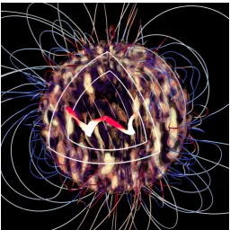
Fig. 3.Non-linear, 3D cyclic dynamo in global turbulent simulations of Strugarek et al. (2017). The rising/sinking convective cells are shown by the dark/bright patches in the convective envelope. A quadrant of the sphere has been cut out (white lines) to reveal the self-consistent generation of strong toroidal magnetic field (red-white ribbon) at the base of the simulated convection zone. A potential extrapolation of the magnetic field outside the star is shown with red/blue tubes labelling magnetic field lines exiting/entering the solar surface.

4.1. Inferring the 3D coronal magnetic field:

The magnetic field is the key player in most (if not all) processes taking place in the solar corona. It permeates all layers of the solar atmosphere, controls the flow and dissipation of energy, and shapes the coronal structures. We discuss in the next sections the challenges faced when modelling the 3D magnetic field.

4.1.1. Some challenges to model coronal magnetic fields:

The magnetic field is difficult to measure in the corona because it is weak and has a complex topology in most cases. Furthermore, the solar corona is optically thin at most wavelength ranges (visible, UV, and EUV) that are relevant to the measurement of the magnetic field.

Several methods show great promise for measuring the field in the low corona and complement each other. They are the Zee-man and Hanle (Hanle 1924) effects and the radio gyroresonance and bremsstrahlung. Radio gyroresonance and bremsstrahlung provide the magnetic field strength and the line-of-sight [LOS] component above on-disk ARs, respectively. Iso-Gauss surfaces can be inferred from the radio emissions but their heights in the solar atmosphere remain ambiguous (Zlotnik 1968; White & Kundu 1997; Lee et al. 1997, 1998; Brosius et al. 1997). Raouafi (2005, 2011) provide comprehensive reviews on the dif-ferent methods used or that can be used to measure the magnetic field directly in the solar corona.

The Zeeman and Hanle effects have been used to obtain di-agnostics of the coronal magnetic field (Harvey 1969; Casini & Judge 1999; Raouafi et al. 1999, 2002; Raouafi 2002). In the near

future, groundbased observatories will be key to exploring the low corona through direct polarimetric diagnostics of the mag-netic field using the Zeeman and Hanle effects. We expect the DL-NIRSP and Cryo-NIRSP instruments of the 4-meter DKIST (Keil et al. 2011) to provide routine measurements of the coro-nal field using these two mechanisms. Other telescopes, such as the COronal Solar Magnetism Observatory (COSMO; Tomczyk et al. 2016), will also contribute significantly. It is now clear that measuring magnetic field in the corona is a prerequisite for un-derstanding global phenomena such as space weather. Ground measurements alone may not be sufficient and the need for a space mission dedicated to this goal is now very obvious.

The Zeeman effect produces a frequency-modulated po-larization signal, which is sensitive to both the direction and strength of the magnetic field. Achieving accurate measurements of the coronal magnetic field through the Zeeman effect is dif-ficult, however, because the magnetic field is weak (typically of the order of 100 G in the strongest field regions above the photospheric imprint of solar active regions), the Zeeman split-ting scales with the wavelength squared, and emission lines have large Doppler widths (Bommier & Sahal-Brechot 1982; Raouafi et al. 2016). Coronal magnetic diagnostics through the Zeeman effect are thus best achieved with infrared spectral lines (Harvey 1969; Kuhn et al. 1996; Judge 1998). More accurate measure-ments have been achieved by Lin et al. (2000, 2004) using the Fe XIII 10747 Åline to measure fields at heights ranging between 1.12 and 1.15 Rfrom sun center. This type of measurements of

coronal field strength via the Zeeman effect suffered from very poor spatio-temporal resolution that is necessary to collect suffi -cient signal in the very weak circular polarization profile. Even at these wavelengths the fraction of circular polarization is only expected to be of the order of 10−4 _{(Querfeld 1982; Plowman}

2014). In such circumstances, measuring circular polarization associated with a 1 Gauss magnetic field in 15 minutes with a 2 arcsec resolution requires larger aperture telescopes, such as the Large Coronagraph (1.5 meter) on COSMO and DKIST.

Even in the best conditions (e.g. choice of spectral lines, large aperture telescopes), determining the 3D solar magnetic field from coronal polarimetry remains a real challenge. Indeed, the solar corona is an optically thin plasma at most wavelengths. Therefore, whether the polarization signal is due to Zeeman, Hanle, or some other mechanism, the signal is the integration of all the plasma emission along the line of sight. As a consequence, it is very difficult to obtain individual coronal magnetic field data at specific positions along the line of sight without stereoscopic observations (Kramar et al. 2013, 2016). Our knowledge of the 3D coronal magnetic field therefore relies on 3D modeling from photospheric and/or chromospheric surface measurements.

The most widely used numerical models that exploit surface vector magnetograms broadly fall into two categories: magneto-static (MHS) and MHD models. The former includes both the Force-Free Field (FFF) models (including potential and current-carrying magnetic fields) which do not consider the plasma and where the electric currents are parallel to the magnetic field lines (e.g., Wheatland et al. 2000; Wiegelmann 2004; Valori et al. 2005; Amari et al. 2006; Contopoulos et al. 2011; Malanushenko et al. 2014), and magnetostatic models which do (Low 1992; Aulanier et al. 1999; Wiegelmann & Neukirch 2006; Wiegel-mann et al. 2007; Zhu & WiegelWiegel-mann 2018). Such magnetostatic solutions are used as initial states to the magnetohydrodynamic models (Miki´c et al. 1999; Inoue et al. 2011; Feng et al. 2012; Zhu et al. 2013). Both these categories include local, i.e. limited to single active regions or to active region groups (e.g., Canou et al. 2009; Gilchrist et al. 2012; Jiang et al. 2014), and full Sun global models (e.g., Titov et al. 2011; Platten et al. 2014; Tadesse et al. 2014; Yeates et al. 2018). In practice, local current-carrying force-free, MHS and MHD models better account for the strong electric currents developing in the vicinity of active regions and are therefore better suited to model their complex magnetic field. Global models provide a full Sun 3D coronal magnetic field that allows to better describe the effects of remote connections be-tween active regions and with the solar wind, and can be used to derive the location and distribution of the suspected source regions of the solar wind (such as helmet streamers, pseudo-streamers, coronal holes). That being said, recent developments have been made to produce global models that also allow to account for the strong electric currents in active regions (e.g., Amari et al. 2018).

Despite all these models, there is currently no unique solu-tion of the 3D coronal magnetic field derived from the photo-spheric measurements. Apart from the fact that such models are built from different assumptions and numerical techniques that inherently result in differences in the final solution, some obser-vational limitations further enhance the lack of ground truth 3D coronal magnetic field. First, photospheric measurements of the transverse magnetic field, which allow to derive the photospheric vertical electric currents, are subject to the 180◦_ambiguity

(Har-vey 1969; Metcalf et al. 2006; Leka et al. 2009). Different meth-ods lead to different ambiguity removal, and hence, different boundary conditions. Second, existing MHS and MHD models do not use the photospheric vector magnetic field in the same manner (e.g., partial vs. full vector, pre-processing for current-carrying FFF models; see e.g., De Rosa et al. 2009), also leading to different boundary conditions. How the boundary conditions deduced from a simulated Solar Orbiter’s PHI instrument influ-ence the quality of 3D magnetic field models has been inves-tigated in Wiegelmann et al. (2010). Third, global models lack of proper boundary conditions. In particular, they require the si-multaneous full 4πsr measurement of the photospheric vector magnetic field, which is not possible from the single vantage

point given by Earth. Full 4πsr vector magnetograms must there-fore be built from non-simultaneous photospheric measurements such as, e.g. synoptic maps (see Section 4.1.2). However, this can have strong effects on global reconstructions of the magnetic field because changes occurring on the invisible or poorly ob-served surface of the Sun can cause strong changes in the global topology of the corona. All these issues directly affect our ability to infer the connectivity of a S/C to the regions where the solar wind forms, as well as to determine whether or not there is a universal threshold for solar flares and CMEs and thus predict them.

For the first time, the Solar Orbiter’s PHI instrument (Solanki et al. 2019) will provide surface magnetic field measurements from outside the Sun-Earth line and from outside the ecliptic plane. Despite possible issues with cross-calibration of magnetic field measurements between different instruments and observa-tories (see e.g., Bai et al. 2014; Riley et al. 2014; Watson et al. 2015), coordinated observations from Earth and Solar Orbiter’s PHI will provide better photospheric boundary conditions for 3D modeling. For instance, observations of the same solar re-gion from both Solar Orbiter’s PHI and Earth’s orbit (via, say, SDO/HMI) can enable the unique removal of the 180◦_ambiguity

in the transverse component of the photospheric magnetic field (Fig. 4, see Section 4.1.2). Solar Orbiter’s PHI vantage point will further provide larger simultaneous photospheric spatial cover-age for global models, reaching its maximum when at 180◦from the Sun-Earth line (although this will be accompanied with the resurgence of the 180◦ambiguity problem). PHI will also allow larger temporal coverage of active regions observed from Earth, providing more complete timeseries of photospheric vector mag-netograms for data-driven models of the 3D coronal magnetic field. Finally, EUV data of coronal loops from EUI will provide more information on the shape of magnetic field lines to help bet-ter constrain 3D magnetic field models (e.g., Malanushenko et al. 2012; Aschwanden 2013). A novel approach, dubbedNonlinear

Force-free Coronal Magnetic Stereoscopyis to combine

mag-netic field extrapolations from vector magnetograms with stere-oscopy from EUV-images (see Chifu et al. 2015, 2017). Using additional observations from out of the ecliptic by EUI will be of great benefit to improve both the stereoscopic 3D-reconstruction of loops and constrain the magnetic field models.

4.1.2. Opportunities to improve magnetograms with Solar Orbiter

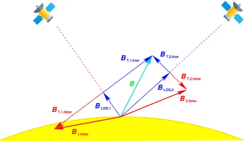
B T,1,true B

BT,1,false

B

B BT,2,false BT,2,true

BLOS,2

LOS,1 B

1,false

2,false

Fig. 4.Sketch of the ambiguity arising by deriving the magnetic field vector using the Zeeman effect. Observations from a single vantage point allows for two different solutions Bor B1,false. Stereoscopic ob-servations make possible the selection of the correct solution between

B,B1,falseandB2,false.

uncertainty with flux transport modeling (e.g., such as the uncer-tainties in the meridional drift or different rotation rates or lack of observations on the solar far-side), the Air Force Data Assim-ilative Photospheric flux Transport (ADAPT) model utilizes an ensemble (with typically 12 realizations) of synchronic synop-tic maps (based on Worden & Harvey 2000) and state-of-the-art data assimilative techniques (see, Hickmann et al. 2015) to rep-resent as realistically as possible the spread in the uncertainty of the state of the global photospheric magnetic field (Arge et al. 2010). The ADAPT global magnetic maps, using the available Earth/L1 perspective magnetograms, are publicly available1_and

used within the heliospheric modeling community, e.g., for time-dependent MHD simulations of the inner heliosphere (Merkin et al. 2016) and ensemble modeling of the large CME during July 2012 (Cash et al. 2015). In addition, ADAPT forecast maps are utilized to predict the observed F10.7 values (i.e., the solar radio flux at 10.7 cm) and bands within the VUV (vacuum ultra-violet, between 0.1 and 175 nm) solar irradiance (Henney et al. 2015). ADAPT maps are also integrated in the operational sup-port for the Solar Orbiter mission (see section 5).

The origin of magnetic forecast maps is given by single pho-tospheric magnetic field maps of the solar disk. Phopho-tospheric vector magnetic field maps obtained from a single vantage point are, however, strongly affected by the 180◦ _{ambiguity of the}

transverse Zeeman effect which leads to an ambiguity of the ob-tained field azimuth with respect to the line of sight and to a big uncertainty of the actual field strength (and even polarity) when transformed to the local, heliographic coordinate system. As only two solutions are possible, observations of the same so-lar region from another vantage point provide the unique oppor-tunity to resolve this ambiguity (see Fig. 4).

Coordinated observations between PHI and, e.g, HMI on-board SDO (see Scherrer et al. 2012) will lead to new methods to produce more realistic vector-magnetograms. Combining ob-servations from two vantage point requires, however, new devel-opments in order to overcome the obvious obstacles for a suc-cessful application of this technique. As shown in Fig. 5 the pri-mary obstacle is the geometric foreshortening and the necessity to cross-correlate observations from different instruments which will be affected by different geometric distortions, spatial res-olution and noise levels which becomes even more relevant as the spatial resolution of PHI changes with Solar Orbiter’s

or-1 _{https://www.nso.edu/data/nisp-data/adapt-maps/}

Fig. 5.MHD simulation of a realistic active region as seem at disk ceter (left panels) and at a heliocentric angle ofθ =60◦

(right panels). The synthesized spectra have been degraded using the instrumental parame-ters of the PHI-HRT telescope at a solar distance of 0.28 AU and subse-quently inverted.

bital position. PHI will sense this effect for the first time in the history of solar magnetography. Although PHI and HMI ob-tain their magnetic fields from observations of the same spec-tral line (Fei6173 Å) the different spectral resolution and helio-centric angles provide observations from different atmospheric heights. As it is well known that the magnetic field structure of the photosphere changes rapidly with height (see e.g. Rempel & Cheung 2014) a careful consideration of this effect is essen-tial and the final goal of such a development must be a com-bined stereoscopic inversion of the radiative transfer equation of both observations (i.e. using data from the PHI raw data obser-vation mode) which intrinsically consider the different forma-tion heights. A comprehensive space-based study of azimuth-disambiguated electric current density from two different angles and spatial resolutions will also provide unprecedented clues to-ward both understanding solar photospheric magnetism and ex-trapolating the photospheric boundary by any modeling means: magnetostatic, magnetohydrostatic, or magnetohydrodynamic -(see, e.g., Georgoulis 2018).

Blanco Rodríguez et al. 2018), assuming PHI-HRT observations at 0.28 AU solar distance, and a subsequent inversion of the ra-diative transfer equation has been carried out with the SPINOR code (Solanki 1987; Frutiger 2000). As the resulting maps of the magnetic field strength are quite comparable the field azimuth already hints to rather different solutions in the two models, e.g. at the left small pore at y = 200. More detailed studies, e.g. including also instrumental parameters of HMI, have to be de-veloped prior to establish a tool to stereoscopically resolve the 180◦ambiguity.

It is also well known that polar regions play a key role for the progression of the solar cycle and, likely, for the underlying dynamo mechanisms (see section 3.4 and, e.g. Charbonneau 2010; Cameron & Schüssler 2015; Petrie 2015). Solar dynamo models, therefore the testing of solar dynamo models, therefore, notably depends on improved vector magnetic field maps of the polar regions. And consequently, also do models that link solar dynamos to the properties of the 3D corona and wind (Pinto et al. 2011; Kumar et al. 2018).

Löptien et al. (2015) list the required observation campaigns and analysis tools allowing to better understand the dynamics of the surface and subsurface layers of the polar regions with measurements carried out by Solar Orbiter. Of particular inter-est is the latitudinal dependence of the large and small scale magnetic field structures and their temporal evolution in order to disentangle contributions from global and local dynamo ac-tions to the global solar magnetic field. In addition, the the mag-netic helicity, as an invariant of ideal magnetohydrodynamics, is assumed to denote a quantity which directly measures the prop-erties of the solar dynamo. Solar Orbiter will allow us to gener-ate improved helicity spectra and their temporal evolution along the solar cycle since during high latitude phases the obtained vector-magnetograms will be less dominated by active regions and false polarity detection because of the 180◦_azimuth

ambi-guity. In order to benefit from the inclined orbit, a study will be performed to determine whether the helicity spectra can be re-trieved from the standard PHI data products or if downloading raw data (Stokes parameters) is required. Ideally, this study will define a dedicated PHI operation mode to compute the helicity spectra onboard PHI as this instrument produces also its standard data products (cf. Albert et al. 2018). Overall it is indeed crucial to link magnetic flux emergence on all scales and latitudes on the solar surface to the internal dynamo mechanism and how these properties vary along the 11-yr cycle, in order to understand how the solar dynamo works in details. Solar Orbiter’s unique orbital trajectory jointly with PHI data measurements will provide such constraints.

4.1.3. Combining surface magnetograms with off-limb coronal polarimetry

Polarimetric measurements in the corona through the Zeeman and Hanle effects (described in section 4.1.1) allow us to diag-nose the strength and direction of the coronal magnetic field. Coronal polarimetry has received more and more attention in the last decade. The Coronal Multichannel Polarimeter (CoMP; Tomczyk et al. 2008) contributed to this field by providing off -limb coronal emission-line polarization measurements in the in-frared through the Fe XIII 10747 and 10798 Å lines. Such mea-surements have been obtained daily since 2011 and are available to the community either through the solarsoft package FOR-WARD (Gibson et al. 2016) or by download from the Mauna

Loa Solar Observatory website2. The circular polarization signal of these two Fe XIII lines is dominated by the Zeeman effect, while the Hanle effect dominates the linear polarization signal (Casini & Judge 1999). While CoMP is mainly sensitive to the linear polarization, coronal circular polarization measurements at these Fe XIII lines will be provided by the Daniel K. Inouye Solar Telescope (DKIST; see Keil et al. 2011, and references therein), which first lights are planned for late 2019.

Theoretical (e.g., Judge et al. 2006; Rachmeler et al. 2013; Dalmasse et al. 2016) and observational (e.g., Ba¸k-Ste¸´slicka et al. 2013; Rachmeler et al. 2014; Gibson et al. 2017) studies have shown that Fe XIII, off-limb coronal polarimetry can dis-tinguish between different 3D magnetic configurations such as, e.g. twisted flux ropes, sheared arcades, streamers, and pseudo-streamers. However, coronal polarimetry alone is not enough to provide the 3D vector magnetic field in the full coronal volume. In addition to the limitations discussed Section 4.1.1, the Hanle effect associated with the Fe XIII lines operates in the saturated regime (Casini & Judge 1999). In other words, the linear polar-ization signal is sensitive to the magnetic field direction but not its strength. Hence, while off-limb coronal polarimetry provides a unique type of information to constrain the vector magnetic field in the full coronal volume, it must be combined with other types of magnetic field measurements (e.g. photospheric or chro-mospheric) that are then integrated into 3D FFF and/or MHD models.

The Data-Optimized Coronal Field Model3 (DOCFM; Dal-masse et al. 2019) proposes such a solution by combining a parametrized FFF model with forward modeling of the coronal polarization signal in the Fe XIII lines. In this framework, the FFF model is parametrized through its electric currents4, which can either be a surface-boundary parametrization for FFF ex-trapolation methods, or a volume parametrization of the coronal electric currents for flux rope insertion methods (e.g., van Bal-legooijen 2004; Titov et al. 2014, 2018). The parametrized FFF model is then optimized by minimizing the mean squared er-ror between the polarization signal predicted for the FFF model and the real polarization signal (e.g. as observed by CoMP). The synthetic polarization signal associated with the FFF model is computed with the solarsoft FORWARD package (Gibson et al. 2016). In a recent study, Dalmasse et al. (2019) present a proof of concept using the flux rope insertion method of van Ballegooi-jen (2004) and CoMP-like data. They show that the DOCFM method opens new perspectives to retrieve the vector magnetic field in the coronal volume by combining off-limb coronal po-larimetry with on-disk surface magnetograms and parametrized FFF models.

For an ideal application of the DOCFM approach, the region of interest must be simultaneously observed from two vantage points, i.e. from atop to obtain the on-disk surface magnetic field, and from the side to measure the corresponding off-limb coro-nal polarimetric signatures. Future coordinated observations of Solar Orbiter with DKIST - when Solar Orbiter is in quadrature with Earth - will thus provide unprecedented opportunities for si-multaneous observations of on-disk surface magnetic fields and off-limb coronal polarimetry. Such measurements will constitute a unique set of observations to test new coronal magnetic field reconstruction techniques, infer the 3D coronal magnetic field of

2 _{https://mlso.hao.ucar.edu/mlso_data_calendar.php?}

calinst=comp

3 _{https://www2.hao.ucar.edu/hao-science/}

data-optimized-coronal-field-model-docfm