Simulated Experiments for Teaching CAD Techniques Using Analytic and Finite Element Solutions of Electromagnetic Two Dimensional Problems with Longitudinal Symmetry

ISSN Online: 1942-0749 ISSN Print: 1942-0730

DOI: 10.4236/jemaa.2019.116006 Jun. 30, 2019 79 Journal of Electromagnetic Analysis and Applications

Simulated

Experiments

for

Teaching

CAD

Techniques

Using

Analytic

and

Finite

Element

Solutions

of

Electromagnetic

Two-Dimensional

Problems

with

Longitudinal

Symmetry

Antônio

Flavio

Licarião

Nogueira,

Rodolfo

Lauro

Weinert,

Leonardo

José

Amador

Salas

Maldonado

Santa Catarina State University, Joinville, Brazil

Abstract

The paper describes an approach to teaching low-frequency electromagnetic CAD techniques to undergraduate students pursuing a degree course in elec-trical engineering. The simulated experiments make use of a two-dimensional open-access software based on the finite-element method. At the laboratory meetings, the problems are initially solved analytically. Upon this, students learn how to create the numeric model and how to define the sequence of field problems that lead to the required solution. Simulation tasks based on a force-producing electromagnet are used to introduce numeric techniques to determine magnetic field distribution, evaluation of energy storage and gen-eration of magnetic forces. The nature of the magnetic force generated in the air gaps of the C-core electromagnet is explained in detail. Magnetic forces are calculated by the classical and weighted versions of the method of Max-well stress tensor. The paper provides all the basic elements required for fur-ther exploration of devices with longitudinal symmetry.

Keywords

Actuators, Electromagnetic Engineering Education, Energy Storage, Finite Element Method, Magnetic Forces

1.

Introduction

The present work aims to encourage higher education teachers to use finite ele-ment programs as a compleele-mentary tool in the teaching of electromagnetics. The enhanced capability of the finite element method in the analysis of problems How to cite this paper: Nogueira, A.F.L.,

Weinert, R.L. and Maldonado, L.J.A.S. (2019) Simulated Experiments for Teach-ing CAD Techniques UsTeach-ing Analytic and Finite Element Solutions of Electromag-netic Two-Dimensional Problems with Longitudinal Symmetry. Journal of Elec-tromagnetic Analysis and Applications, 11, 79-99.

https://doi.org/10.4236/jemaa.2019.116006

Received: April 16, 2019 Accepted: June 27, 2019 Published: June 30, 2019

Copyright © 2019 by author(s) and Scientific Research Publishing Inc. This work is licensed under the Creative Commons Attribution International License (CC BY 4.0).

DOI: 10.4236/jemaa.2019.116006 80 Journal of Electromagnetic Analysis and Applications involving non-homogeneous, non-linear and time-dependent problems has been determinant in the choice of this numerical method. The manuscript takes the reader to a step-by-step simulation journey that provides all the basic elements required for the analysis of electromagnetic devices with longitudinal symmetry. It is worth noting that many practical electrical devices like motors, transformers and actuators possess longitudinal symmetry. The work will certainly benefit higher education teachers who intend to create new virtual laboratories or to in-troduce changes in the existing ones. A similar work for the exploration of axi-symmetric problems has been recently published and appears in [1]. Both papers contain a section devoted to the numeric modeling of the test problem that can serve as a template for future simulation practices on new topics.

Following the high impact of the first application of the finite element method in electrical engineering in 1969, industrial researchers and academic groups soon realized the need for training courses offered to designers and postgraduate students in order to overcome the difficulties in using such a versatile tool in industrial design and education.

There have appeared many papers describing experiences on the use of the fi-nite element method in the teaching of electromagnetics. Some papers describe the experience of academic groups in the development of their electromagnetic field simulators, and explain how these programs have been used as teaching tools [2]. Commercial finite element packages have also been successfully used as an aid in teaching electromagnetics around the world. The main disadvantage of commercial packages is the expensive licensing. In their work, Lowther and Freeman describe how laboratory courses on field simulation based on a com-mercial software have been devised and implemented in three different universi-ties, and discuss the advantages and disadvantages of finite-element CAD tools in the teaching environment [3].

At the turn of the century, open-access programs based on the finite element method have been released, and many of these programs have been used as teaching tools [4] [5] [6]. As a result, a limited and free of charge students’ ver-sion of commercial packages also started to be released. To make their product even more competitive, some companies have also allowed free access to a series of files containing lecture notes, problem workshops and tutorials based on the limited version of their software [7] [8]. In their experience in teaching electro-magnetics, Yin et al. have used a combination of two commercial simulation packages and in-house developed software [9].

DOI: 10.4236/jemaa.2019.116006 81 Journal of Electromagnetic Analysis and Applications and their familiarity with that mathematical tool has been the principal reason for the creation of MATLAB-based electromagnetic-fields virtual laboratories [14] [15]. The use of finite element methods in the teaching of electromagnetics is a topic of great interest, and new contributions to the art appear very often in specialized magazines [16], scientific journals [17] [18] and conference pro-ceedings [19] [20] [21] [22].

The discussion presented in the following is based on the authors’ teaching experience in the context of a thirty-hour course. The activities include 6 hours of lectures and 24 hours of laboratory classes. The object of the introductory lectures is to present basic concepts of the finite element method: domain dis-cretization, use of simple boundary conditions, polynomial trial functions, and formulation of the system of equations. The lectures are followed by a series of laboratory meetings where analytical calculations and field computations are made on simple physical devices. One of these meetings focuses on the creation of the numeric model of a force-producing electromagnet. This numeric model is employed in six simulated experiments chosen to introduce numeric tech-niques to determine magnetic field distribution, evaluation of magnetic energy storage, generation of magnetic forces and eddy current losses.

2.

The

Test

Problem

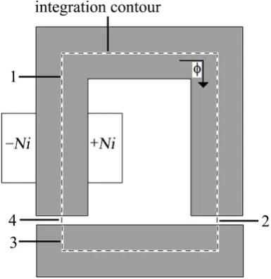
To make the matter concrete, the step-by-step description of the numeric model for planar problems is based on the same device that appears in the simulated experiments: the C-core electromagnet shown in Figure 1. The magnetic force generated in this device attracts the movable rectangular armature into the C-core electromagnet.

In the illustration, lg denotes the length of the two small air gap regions that

separate the movable armature from the stationary core. The winding has 250 turns and an intrinsic resistance of 7.5 Ω. In the dc operation, it carries a current of 5.33 A. In the ac operation, the peak current is also 5.33 A.

DOI: 10.4236/jemaa.2019.116006 82 Journal of Electromagnetic Analysis and Applications The electromagnet shown in Figure 1 represents one of the simplest devices that produce electromechanical forces, and has long been used to teach methods of magnetic force calculation. Two of the most popular types of linear actuators have stationary cores in the shape of “C” and “E”, and are commonly referred to as C-core and E-core actuators, respectively. A C-core actuator has been chosen by Kim, Lowther and Sykulski [23] to evaluate the accuracy of force computa-tion algorithms to determine global forces, as well as force distribucomputa-tion over the surfaces of magnetized bodies in contact. Different types of C-core actuators have also been used to demonstrate applications of the single-solution virtual work method [24].

3. Analytical Methods

Analytical calculations are important because they bring insight into the subject. When applied to devices with simple geometries, they can provide very accurate or even exact estimates of the quantity under investigation. It is the case of the analytic estimates of the magnetic field strength and attractive force of the C-core electromagnet described in Section 2. In problems involving more com-plicated slotted magnetized structures, all that can be expected from an analyti-cal solution is to establish the order of magnitude of the quantity under investi-gation. The main disadvantage of analytical calculations is the lack of flexibility in accommodating alterations in the device’s geometry, its sources and design constraints.

Analytical calculation of global parameters like stored energy, inductance and total forces are usually based on equivalent magnetic circuits containing the sources of magnetomotive forces and a number of interconnected reluctors crossed by the “circulating” magnetic fluxes. These circuits are used together with magnetic Ohm’s law and Ampère’s law to determine the approximate mag-nitude and direction of the magnetic field strength H or magnetic induction B in the regions of interest. In our simplified analytical approach, the iron sections of the device are modelled by assuming a high constant relative permeability, µr, in

the x and y directions. As a result, the problems are treated as magnetically li-near, and the magnetic energy storage is considered to be entirely confined to the air regions.

3.1.

Ampère’s

Law

In the analysis of simple devices like the electromagnet shown in Figure 1, the terminal current i and the number of turns N of the exciting winding are usually known, and Ampère’s law provides a method for determining the magnitude of the H-field,

d Ni.

⋅ =

∫



in-DOI: 10.4236/jemaa.2019.116006 83 Journal of Electromagnetic Analysis and Applications tegration contour indicated in (1) should be formed by the union of line-segments that cross the magnetized parts and air gaps in a way that the H-field is tangen-tial to each segment or contour section. In the illustration of Figure 2, each part or section of the integration contour is related to a number: section “1” follows the mean path of the stationary C-core; Sections 2 and 4 follow the mean path of the air gaps; and Section 3 follows the mean path of the movable armature.

Along each of the paths that form the integration contour, the magnitude of the H-field is more or less constant, the field direction is almost tangential to the path, and the integration can be approximated by the summation

4

1 k k

k= H l Ni

=

∑

where k represents the number of the contour section.

Under idealized conditions, the magnitude of the H-field and related magne-tomotive force drops Hl along the iron sections 1 and 3 of the integration con-tour shown in Figure 2 are negligible, so that

1 1 2 2 3 3 4 4

0 0

. H l H l H l H l Ni

→ →

+ + + = ₍₃₎

If the two air gap regions have the same geometric dimensions, H2 =H4 =Hg. If lg denotes the length of one air gap, the estimate for the uniform magnetic

field, Hg, in the air gap regions is computed by

. 2

g g

Ni H

l

= (4)

Once computed the magnitude of the magnetic field in the air gaps, the calcu-lation of the attractive force can be easily performed using the method of Max-well stress tensor.

DOI: 10.4236/jemaa.2019.116006 84 Journal of Electromagnetic Analysis and Applications

3.2.

The

Maxwell

Stress

Tensor

Method

Figure 3 contains an enlarged view of the actuator’s right-hand side air gap. In smooth magnetized surfaces, like the ones that form the millimetric gaps of this actuator, the H-field practically does not vary in magnitude from point to point, and its direction is perpendicular to each iron surface. For a magnetic flux φ

crossing the gap in the -y direction, the magnetic field intensity H emerges from the upper iron-air interface and penetrates the lower iron-air interface. To cal-culate the net force by integration of the Maxwell stress tensor method, it is firstly necessary to compute the distribution of the magnetic field in terms of the H- (or B-field) at all points in the air region surrounding the object on which the force is to be calculated. In the calculation of the total force acting on a rigid body, the integration surface S could be the surface of the body itself. In compu-tational practice, however, the use of a “surface of air” attached to the iron sur-face overwhelmingly facilitates the calculation. The area S of this surface of air is usually taken as the magnetic section of the magnetic pole, as indicated in the il-lustration. At any point of a given interface, the angle between the local force density vector dp and the surface vector dS—taken as the outward normal on the surface—is the double of the angle between the local magnetic field strength H and the surface vector dS. In this particular situation, vectors dp and dS are collinear on the two iron-air boundaries facing each other. As a result, the ele-mental local force density vector dp is directed downwards in the upper iron-air interface and upwards in the lower iron-air interface. In the illustration, the small arrows emerging from the two artificial layers of air represent the uniform distribution of the elemental force density vector dp.

The above discussion helps to explain the nature of the attractive force gener-ated at the air-gap region. The resulting magnetic force always tends to shorten the length of the air-gap and its value is computed by means of the surface integral of the local force density vector dp over one surface of air. According to Newton’s first law, the force acting on the opposite iron-air surface has the same magnitude and opposite direction.

DOI: 10.4236/jemaa.2019.116006 85 Journal of Electromagnetic Analysis and Applications In two-dimensional analysis, when magnetic forces are calculated by the me-thod of Maxwell stress tensor, the surface of integration becomes a contour of integration. In this example, the contour of integration should encompass the movable armature, and the choice of this contour affects the accuracy of com-puted forces. This happens because the comcom-puted field distribution, expressed in terms of the H- or B-field, is only an approximation to the true or “perfect” one, i.e., there is an inherent error in the numerical field distribution, and the inde-pendence of the values of computed forces relative to the choice of the integra-tion contour disappears. To overcome the difficulties encountered in choosing integration contours to get accurate and consistent force calculations from im-perfect numerical field solutions, McFee, Webb and Lowther [25] have proposed the method of weighted Maxwell stress tensor method. Despite the complexity of its mathematical derivation, the weighted approach became an essential simula-tion tool of modern electromagnetic CAD systems, wherein the contours of in-tegration and weighting functions are calculated in a completely automated process. The post-processing tasks necessary to use this method are presented in Experiment No 4.

4.

Finite

Element

Model

4.1.

Advantages

and

Disadvantages

of

the

Method

The finite element method is a numeric technique based on the theory of inter-polations to solve large-scale problems of high complexity employing a data structure that is, at the same time, simple and flexible. As a result, programs de-veloped for a particular discipline can be applied to solve problems in a different field with little or no modification. The main advantage of the method is its en-hanced capability to solve problems involving: 1) complex geometries; 2) non-linearities; 3) non-homogeneous media and 4) time-dependent phenomena. The typical unstructured finite-element meshes allow good representation of curved objects, easy insertion of short gaps as well as increased local resolution in regions wherein rapid variations of the solution are expected to occur.

Despite its worldwide popularity, the method of finite elements has disadvan-tages, and these include its rigorous mathematical derivation as well as the use of a large amount of input and output data. The method does not produce a gener-al closed-form solution, but only an approximate solution to the numeric model. The construction of a finite-element model invariably involves several us-er-defined parameters and numerous choices that affect the accuracy and con-sistency of the finite element solutions. In other words, different numeric models for a given problem may lead to different results, so the quality of the finite ele-ment simulations rely heavily on the experience of the user in constructing a fi-nite element model “adequate” to the problem. Besides, experience and judg-ment are needed to extract and examine the results.

4.2.

Problem

Definition

and

Geometry

DOI: 10.4236/jemaa.2019.116006 86 Journal of Electromagnetic Analysis and Applications simulation software based on the finite element method [4]. The work involves one numeric model and a set of problems defined on that model. The study in-volves a set of problems of magnetism, so it is necessary to select the solver for magnetics problems and, implicitly define the primary quantity of calculation, that is the magnetic vector potential A. In the two-dimensional analysis of prob-lems with translational symmetry, the magnetic vector potential A possesses on-ly a single component in the longitudinal or z-direction, and may be treated as a scalar quantity A.

The selection of the type of symmetry to be exploited—longitudinal in the case of planar problems—is followed by the identification of the length unit as-sociated with the dimensions prescribed in the model’s geometry. In problems with longitudinal symmetry, care must be taken to specify the “depth” parameter. The value prescribed to this parameter—in the same length unit selected for the model’s geometry—represents the length of the device in the “into the page” di-rection.

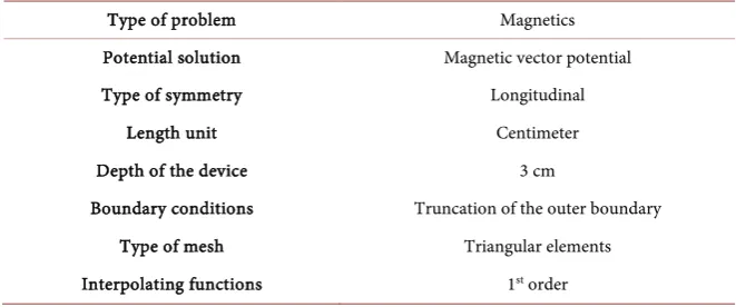
An outline of the numerical model with geometrical dimensions in centimeter is shown in Figure 4. The external rectangular region that appears in the illu-stration is an artificial boundary used to close the domain of analysis. The boundary conditions applied to this rectangular boundary are truncation of the outer boundaries. This technique assumes that no magnetic flux φ _{crosses the}

boundary in the normal direction. The usual way of applying this mathematical condition is by prescribing A = 0 at this boundary. The main features of the nu-meric model are summarized in Table 1.

DOI: 10.4236/jemaa.2019.116006 87 Journal of Electromagnetic Analysis and Applications Table 1. Features of the finite-element model.

Type of problem Magnetics Potential solution Magnetic vector potential Type of symmetry Longitudinal

Length unit Centimeter Depth of the device 3 cm

Boundary conditions Truncation of the outer boundary Type of mesh Triangular elements Interpolating functions 1st _order

4.3.

Problem

Assembly

The subdivision of the geometric domain into regions or “blocks” must consider the need of extra degree of mesh fineness in small air-gap regions and pole tips, as well as the need of separately quantifying the energy storage in some regions or areas of the device. In this particular actuator, one single region could be used to model all regions filled by air. However, this would not allow computing the amount of energy storage restricted to each small air-gap region, as required by some force calculation methods.

The proposed finite-element model contains eight regions, and these regions must be correlated to different material media. Initially, a label must be placed in each region, and this label will identify all triangular elements belonging to that region or “block”. The disposition of region labels in the geometric domain is il-lustrated in Figure 5(a). Labels “X1”, “X2”, “X3” and “X4” are placed in the re-gions that model the two air gaps, the stator window, and the external area of empty space, respectively. In the same manner, labels “Y1” and “Y2” are placed in the two non contiguous regions that represent the winding, and labels “Z1” and “Z2” are placed in the regions that model the stator and movable armature, respectively. Up to this point, the region labels are abstract entities, not yet de-fined. To carry on the problem assembly, it is necessary to associate material properties with region labels.

DOI: 10.4236/jemaa.2019.116006 88 Journal of Electromagnetic Analysis and Applications Figure 5. (a) Disposition of region labels; (b) Correlation

between region labels and materials data files.

It is worth noting that files of material properties may contain a large amount of information. Whereas the data file related to free space or “air” only provides the value of relative magnetic permeability of the material medium (µr x, =µr y, =1),

the data file of a soft magnetic material may contain all necessary information to fully characterize the ferromagnetic core of a power transformer, i.e., 1st

qua-drant B-H curve, loss curves, maximum relative permeability, electric conduc-tivity, lamination thickness and lamination fill factor. Certainly, some familiarity with soft magnetic materials used in industry is important to future engineers. Experiment N˚ 6 takes this fact into account.

4.4.

Exciting

Winding

The winding is modeled by the two non contiguous rectangular regions shown in Figure 5(a). These regions are identified by labels “Y1” and “Y2”. A “circuit property” must be assigned to both conductive regions. For a given circuit prop-erty, it is necessary to specify the magnitude of the terminal current and the winding’s number of turns. In addition, both conducting regions must be de-fined as series-connected.

en-DOI: 10.4236/jemaa.2019.116006 89 Journal of Electromagnetic Analysis and Applications force a magnetic flux φ in the clockwise direction, the specified number of turns is +250 for the left-hand side region and −250 for the right-hand side region. The sign on the number of turns indicates the direction of current flow asso-ciated with a positive-valued circuit current. According to the convention of this field simulator, a positive-valued circuit current flows in the “out-of-the-page” direction.

4.5.

Mesh

Refinement

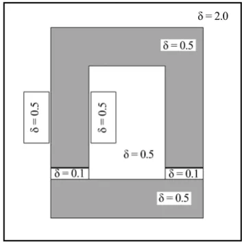
The labels placed in the different regions of the model are also used in the dialog that defines the “grain” of the mesh in one or more selected regions. The method employed to control the level of discretization in each region is based on the specification of a parameter, δ, known as “edge size”. This parameter defines a constraint on the largest possible size of the elements’ edges allowed in that re-gion. Values prescribed to this parameter in the eight regions of the model are indicated in the illustration of Figure 6.

Figure 7(a) contains a view of the right-hand side air gap and adjacent re-gions. Two enlarged views of the small rectangular region highlighted in the il-lustration are used to show the effect of mesh refinement. Figure 7(b) shows the coarse mesh created when the mesh generator is free to choose all elements’ size, whilst Figure 7(c) shows the result of the mesh refinement guided by the speci-fied values of the parameter δ.

5.

Experiments

5.1.

Experiment

1:

Magnetic

Force

at

dc

Operation

Consider the C-core electromagnet shown in Figure 1. A constant terminal vol-tage E = 40 V is applied to the exciting winding. Use the analytic formulae pre-sented in Section 3 and determine the attractive magnetic force acting on the movable armature.

DOI: 10.4236/jemaa.2019.116006 90 Journal of Electromagnetic Analysis and Applications Figure 7. (a) Enlarged view of the right-hand side

air gap; (b) Coarse mesh; (c) Refined mesh.

5.2.

Solution

to

Experiment

1

In dc operation, the inductive reactance XL= jwL of the electric circuit is null,

and the current is only limited by the resistance of the winding. The terminal current I is constant and computed by Ohm’s law,

5.33 A. E

I R

= = (5)

Under idealized conditions, Ampère’s law provides an estimate for the statio-nary and uniformly distributed magnetic field strength Hg in the two air gap

re-gions,

3

250 5.33 666.25 kA m,

2 2 10

g g

NI H

l −

×

≅ = =

× (6)

where lg denotes the length of one air gap.

In both air gaps, the force density vector p is uniformly distributed, and its magnitude is computed by

2 2 0 ₂g N m .

H

p=

µ

If S denotes the stator’s magnetic section, the attractive force Fg in one air gap

is given by the product pS,

2

0 ₂g N.

g

H

F =

µ

The total force, F, attracting the movable armature is the double,

( )

0 2

2 .

4

g

g

NI

F F S

l µ

DOI: 10.4236/jemaa.2019.116006 91 Journal of Electromagnetic Analysis and Applications Substitution of numeric values gives F = 503 N for the idealized force calcula-tion. It is worth noting that the magnetic force varies with the magnetic field in-tensity squared. Under idealized conditions and for a giving magnetomotive force NI, (4) yields the highest estimate for the air-gap field intensity and (9) produces the highest estimate for the attractive force acting on the movable ar-mature. Computation of the attractive force under non idealized conditions will be subject of analysis on Experiment N˚4.

5.3.

Experiment

2:

Relative

Permeability

and

Tangential

H

-Field

One of the most important properties of ferromagnetic materials is their large relative permeability µr. Iron with 0.2% impurities has a relative permeability of

about 6000, and some alloys reach a relative permeability of 106_{. For a given}

ex-citation Ni, the idealized analytic calculations assume that the magnetic field in-tensity, H, is null in the magnetized parts of the electromagnet and, therefore (4) yields the highest estimate for the magnetic field intensity, Hg, in the air gaps. To

investigate what happens in computational practice, two similar problems may be defined on the numeric model. The only feature differentiating the two mag-netostatic problems is the relative permeability of the soft magnetic material used in the magnetic core: 1018 Steel in the first solution and M-36 Steel in the second one. The corresponding values of the relative permeabilities are: µr = 529

for the 1018 Steel, and µr = 1,616 for the M-36 Steel. In the investigation, the

quantity of prime interest is the tangential component, Htan, of the magnetic field

intensity.

5.4.

Solution

to

Experiment

2

To facilitate the analysis, the magnetic portions of the electromagnet, stator and armature, are treated as non laminated, isotropic and magnetically linear mate-rials. The relative permeability of isotropic materials has the same value in all directions and, in a two-dimensional analysis, µrx =µry. Under the assumption of magnetic linearity, the value of the relative permeability is constant, and does not vary with the magnetic field intensity. In the numeric model, properties of the two selected soft magnetic materials should be associated with labels Z1 and Z2: 1018 Steel in the first problem and M-36 Steel in the second one. Both ma-terial data files must be edited to enforce the option “Linear B-H relationship”. By doing this, the value corresponding to the steepest slope of the non linear B-H data set, known as maximum relative permeability, will be attributed to the relative permeabilities µrx and µry in all subsequent calculations.

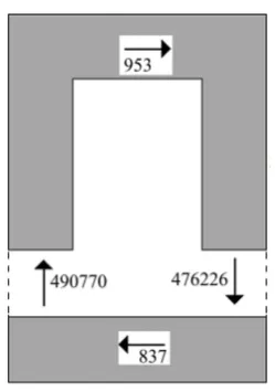
Mean values of the H-field tangential component along the integration con-tour shown in Figure 2 are summarized in Table 2. For the first problem, the averaged values of the tangential H-field along the contour are shown in Figure 8. In the mean, the magnitude of the tangential component, Htan, in the two

magnetic sections is only 0.2% of the averaged magnitude of the tangential component, Htan, in the two air gaps. A careful observation of the results

DOI: 10.4236/jemaa.2019.116006 92 Journal of Electromagnetic Analysis and Applications Figure 8. Averaged tangential H-field

when the core material is 1018 Steel.

Table 2. Mean value of the tangential H-field in units of A/m.

Region Core material and relative permeability Analytic calculation 1018 Steel, µr = 529 M-36 Steel, µr = 1,616

Stator 953 389 0

Right gap 476,226 584,362 666,250

Armature 837 342 0

Left gap 490,770 599,013 666,250

even more pronounced when the core is made of the more “permeable” material M-36 Steel. As the relative permeability increases from 529 to 1,616, the ratio of the tangential H-fields in the two material media decreases from 0.2% to 0.06%. This helps to explain why in many simplified analytic calculations no attempt is made to compute the magnitude of the tangential H-field in the magnetic sec-tions.

5.5.

Experiment

3:

Energy

Storage

in

Magnetic

Materials

Investigate how the relative permeability of the material employed in the ferro-magnetic core affects the storage of ferro-magnetic energy in the ferroferro-magnetic core and air-gap regions.

5.6.

Solution

to

Experiment

3

DOI: 10.4236/jemaa.2019.116006 93 Journal of Electromagnetic Analysis and Applications For this, a series of new material data files have been created, each one contain-ing a filename and values of the relative magnetic permeability in the x- and y-directions. To facilitate the future use of these materials files, the filename suggests the value of the relative permeability. For example, filename Mu_r 500 suggests a materials data file for a soft magnetic material with relative permea-bility µr = 500 in the x- and y-directions.

When post-processing the finite-element solutions, it is necessary to quantify: 1) the energy stored in the ferromagnetic core; 2) the energy stored in the two air gaps; and 3) the energy stored in the whole geometric domain. The effect of an increasing magnetic relative permeability on the amount of energy stored in the ferromagnetic core and air gaps is presented in the graph of Figure 9. The cha-racteristic plotted using a solid line represents the percent stored energy in the ferromagnetic core, whilst the characteristic with circular marks represents the percent stored energy in the two millimetric gaps. Observation of former cha-racteristic shows a pronounced decay of the energy stored in the ferromagnetic core along the leftmost portion of the curve: as the relative permeability increas-es from 500 to 4,000, the percent stored energy in the ferromagnetic core drops from 27% to 4.5%. This variation ought to be compared to the simultaneous in-crease, from 60% to 80%, in the useful, force-producing stored energy in the two air-gap regions.

5.7.

Experiment

4:

Relative

Permeability

and

Magnetic

Force

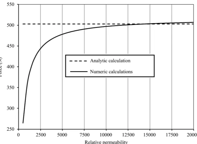
Investigate how the relative permeability of the material employed in the ferro-magnetic core affects the value of the ferro-magnetic force acting on the movable ar-mature when the exciting winding is supplied by a dc current of 5.33 A. The magnetically produced forces must be evaluated numerically, using the numeric method of weighted Maxwell stress tensor.

5.8.

Solution

to

Experiment

4

The first step of the investigation is the definition of a sequence of similar prob-lems with increasing values of the core’s relative permeability. Like in experi-ment N˚3, value of the relative permeability varies from 500 to 20,000, in steps of 500. Once the sequence of problems has been generated, it is necessary to launch the solver and then inspect the results. The post-processing of each fi-nite-element solution involves three main steps, to know: 1) the block or region that represents the movable armature must be selected; 2) the “surface integral” command must be selected; and 3) the task “force via weighted stress tensor” must be chosen from the drop list.

DOI: 10.4236/jemaa.2019.116006 94 Journal of Electromagnetic Analysis and Applications Figure 9. Percentage of stored energy: 1) in the ferromagnetic core: solid line; 2) in the air gaps: circular marks.

Figure 10. Computed forces versus relative permeability.

DOI: 10.4236/jemaa.2019.116006 95 Journal of Electromagnetic Analysis and Applications the second region. For relative permeabilities close to 11,000, the ferromagnetic core is already heavily saturated. As a result, the magnetic field strength at the gaps and the resulting attractive force converge to the values computed analyti-cally by (6) and (9), respectively. For relative permeabilities greater than 11,000, the percent error between numeric and analytic force calculations is less than 1%, i.e., numeric and analytic calculations of the attractive force are computationally equivalent.

5.9.

Experiment

5:

Magnetic

Force

at

ac

Operation

Consider the C-core electromagnet shown in Figure 1. The exciting winding is supplied by an ac sinusoidal current at the operating frequency of 60 Hz. The peak value, Ip, of the terminal current is 5.33 A, the same value of the terminal

current at the dc operation. Use the analytic approach and determine the attrac-tive magnetic force acting on the movable armature for this operating condition.

5.10.

Solution

to

Experiment

5

When the exciting winding is supplied by an alternating current, the magnetic field strength H alternates and so does the force density vector p. If Ip denotes

the peak value of the ac current, the instantaneous current is

( )

( )

i t =I ωt (10)

and the magnitude of the force density vector in the two air-gap regions is com-puted by

( )

2 2

2

0 ₈ 2 N m .

g

n i t p

l

µ

= (11)

The instantaneous force density vector can be expressed, either in terms of the fundamental angular frequency ω as

( )

( )

0 ₈ 2 cos N m ,

p

g

n I

p t t

l

µ ω

= (12)

or in terms of the double angular frequency 2ω,

( )

(

)

0 ₈2 1 1 cos 2_{2 2} N m .

p

g

n I

p t t

l

µ  ω 

= _ + _

  (13)

The product of the force density times the area S gives the attractive force in one air gap. For two air gaps, the value ought to be doubled. The alternating at-tractive magnetic force F (t) acting on the movable armature is thus given by

( ) ( )

(

)

1 1

2 cos 2 N.

2 2 8

p

g

n I

F t S t

l

µ  ω 

= _ + _

  (14)

Substitution of numeric values yields the following expression for the double-frequency attractive force:

( )

(

)

DOI: 10.4236/jemaa.2019.116006 96 Journal of Electromagnetic Analysis and Applications In the graph of Figure 11, one can identify three important features of the si-nusoidal characteristic that represents the double-frequency magnetic force: 1) its peak value is equal to fdc, the value of the stationary dc magnetic force,

represented in the graph by the horizontal solid line; 2) its minimum value is zero; 3) its mean value, represented by the horizontal dashed line, is equal to fdc/2, half the value of the dc magnetic force.

It is worth noting that the alternating magnetic field due to the exciting winding generates an alternating attractive force that drops to zero twice each cycle of the driving alternating current. This would cause undesired mechanical vibration of the magnetized parts and metallic contacts attached to the actuator at the “closed” position. In practice, this does not happen. Industrial ac actuators and contactors contain restoring springs and shading rings designed in a way that the net attractive force never drops below the mechanical forces created by the restoring springs. The reduction of the flux due to the exciting winding oc-curs simultaneously to the increase in the magnetic flux due to the currents in-duced in the shading rings, so that the circulating magnetic flux never drops to zero. A detailed discussion on the combined effect of the fluxes provided by the ac exciting winding and shading rings may be found in [26].

5.11.

Experiment

6:

Eddy

Current

in

Laminated

Cores

Most electric power equipment employ cores built up out of thin laminations in the attempt to reduce eddy current effects. To gain some experience on the analysis of electric devices used in real-world engineering, specify the core of the electromagnet as a laminated structure. Use the built-in library to choose the material employed in the laminations. Try to find a soft magnetic material with maximum relative permeability higher than 1,000. The peak value of the 60-Hz exciting terminal current is 5.33 A. The quantity of prime interest in the analysis is the eddy current loss.

5.12.

Solution

to

Experiment

6

Data files for soft magnetic materials are found in separate file directories, to know: 1) Low Carbon Steel; 2) Magnetic Stainless Steel; 3) Silicon Iron; 4) Cobalt Iron; and 5) Nickel Alloys. The first material used in Experiment N˚ 2, the 1018 Steel, belongs to the family of “low carbon steels”, and may be disregarded be-cause its maximum relative permeability is only 528. The second material, the M-36 Steel, belongs to the family of “silicon irons”, and satisfies the problem’s constraint: its maximum relative permeability is µr = 1,616. Other special

attributes of the M-36 laminated structure include: the electric conductivity of the lamination σlam = 2.0 MS/m, the thickness of each lamination Tlam = 0.635

mm, and the fill factor of the pack of laminations, FFlam = 0.98 per unit. If only

DOI: 10.4236/jemaa.2019.116006 97 Journal of Electromagnetic Analysis and Applications Figure 11. Variation of ac and dc magnetic forces.

When post-processing the field solution, it’s necessary to choose the task “to-tal losses” from the drop list related to the numeric surface integration over the ferromagnetic core. This experiment illustrates an application wherein eddy currents are restricted by lack of space, not by the high resistivity of the core’s material. For this problem, the eddy current loss amount to 1.31 watt, and this represents only 0.6% of the apparent power input. This level of power loss is completely satisfactory for most practical design constraints.

6.

Conclusion

The work discusses the use of finite element programs as a complementary tool in the teaching of electromagnetics. All simulations in the virtual laboratory make use of a two-dimensional open-access software. An important aspect of the laboratory of simulations is its library of simulated experiments. Considerable time and effort is necessary to build and maintain a library of simulated experi-ments. The library must be updated periodically, and new experiments must in-corporate the enhancements of the field simulator. To reach efficient and effec-tive training, qualitaeffec-tive and quantitaeffec-tive issues have to be considered when planning the activities in the laboratory of simulations. A small number of as-signed experiments may take the students to draw simple conclusions restricted to a particular class of problems. On the other hand, the indiscriminate use of a very large number of experiments may result in an exhaustive activity that ad-versely interferes with the time students need for exercising their creativity and thinking deeply during the laboratory classes and homework.

Acknowledgements

Thanks are given to David Meeker for the use of the electromagnetic field simu-lator FEMM (http://www.femm.info/wiki/HomePage). Thanks are also due to the Brazilian Federal Agency for Postgraduate Studies (CAPES), for the spon-sored access to several scientific web sites.

Conflicts

of

Interest

DOI: 10.4236/jemaa.2019.116006 98 Journal of Electromagnetic Analysis and Applications

References

[1] Nogueira, A.F.L., da Costa, V.H.P. and Weinert, R.L. (2017) Simulated Experiments for Teaching Mutually-Coupled Circuits CAD Techniques Using Analytic and Fi-nite Element Solutions. Journalof Electromagnetic AnalysisandApplications, 9, 183-202. https://doi.org/10.4236/jemaa.2017.911016

[2] Trlep, M., Hamler, A., Jesenik, M. and Stumberger, B. (2006) Interactive Teaching of Electromagnetic Field by Simultaneous FEM Analysis. IEEE Transactions on Magnetics, 42, 1479-1482. https://doi.org/10.1109/TMAG.2006.871437

[3] Lowther, D.A. and Freeman, E.M. (1993) A New Approach to Using Simulation Software in the Electromagnetics Curriculum. IEEETransactionsonEducation, 36, 219-222. https://doi.org/10.1109/13.214701

[4] Meeker, D.C. (2019) Finite Element Method Magnetics, User’s Manual, Version 4.2.

http://www.femm.info/wiki/HomePage

[5] Baltzis, K.B. (2008) The FEMM Package: A Simple, Fast, and Accurate Open Source Electromagnetic Tool in Science and Engineering. JournalofEngineeringScience andTechnologyReview, 1, 83-89. https://doi.org/10.25103/jestr.011.18

[6] Tera Analysis Ltd. (2018) QuickField: Finite Element Analysis System. User’s Guide, Version 6.3.2. http://quickfield.com/downloads/quickfield_manual.pdf

[7] Emson, C.R.I. and Edwards, J.D. (2008) Using Commercial Design Software as an Aid for Teaching Electromagnetics. 2008 IET 7th International Conference on Computation in Electromagnetics, Brighton, 7-10 April 2008, 68-69.

https://doi.org/10.1049/cp:20080225

[8] Mentor: A Siemens Business. Products & Solutions.

https://www.mentor.com/products/mechanical/magnet/magnet/

[9] Yin, W.-L., Zhao, Q., Zhang, K. and Qu, Z.-G. (2018) New Developments in Teaching Electromagnetics through Advanced Numerical Simulations and Virtual Experiments. CreativeEducation, 9, 2878-2883.

https://doi.org/10.4236/ce.2018.916216

[10] Rossi, L.N., Silva, V.C., Martinho, L.B. and Cardoso, J.R. (2008) A Geometrical Ap-proach of 3-D FEA for Educational Purposes Applied to Electrostatic Fields. IEEE TransactionsonMagnetics, 44, 1674-1677.

https://doi.org/10.1109/TMAG.2007.916164

[11] Cardoso, J.R. (2016) Electromagnetics through the Finite Element Method: A Sim-plified Approach Using Maxwell’s Equations. CRC Press, Boca Raton.

https://doi.org/10.1201/9781315366777

[12] Özgün, Ö. and Kuzuoglu, M. (2018) MATLAB-Based Finite Element Programming in Electromagnetic Modeling. CRC Press, Boca Raton.

https://doi.org/10.1201/9780429457395

[13] Sadiku, M.N.O. (2018) Computational Electromagnetics with MATLAB. 4th Edi-tion, CRC Press, Boca Raton. https://doi.org/10.1201/9781315151250

[14] Markovic, M. (2013) Computer Aided Teaching and Learning in an Undergraduate Electromagnetics Class. Proceedingsofthe 2013 AmericanSocietyforEngineering EducationPacificSouthwestConference,Riverside, 18-20 April 2013, 583-603. [15] Song, S.H., Antonelli, M., Fung, T.W.K., Armstrong, B.D., Chong, A., Lo, A. and

Shi, B.E. (2018) Developing and Assessing MATLAB Exercises for Active Concept Learning. IEEETransactionsonEducation, 62, 2-10.

https://doi.org/10.1109/TE.2018.2811406

DOI: 10.4236/jemaa.2019.116006 99 Journal of Electromagnetic Analysis and Applications Tu, K.-M., Lin, H.-C. and Peng, S.-T. (2016) Promoting Effective Education in Electromagnetics. IEEEAntennas&PropagationMagazine, 58,99-129.

https://doi.org/10.1109/MAP.2015.2501228

[17] Browne, D.R., Flint, J.A. and Pomeroy, S.C. (2012) Implementing a Mobile Virtual Electromagnetics Laboratory. IET Science, Measurement and Technology, 6, 398-402. https://doi.org/10.1049/iet-smt.2011.0122

[18] Notaroš, B., McCullough, R., Manić, S.B. and Maciejewski, A.A. (2019) Comput-er-Assisted Learning of Electromagnetics through MATLAB Programming of Elec-tromagnetic Fields in the Creativity Thread of an Integrated Approach to Electrical Engineering Education. Computer Applications in Engineering Education, 27, 271-287. https://doi.org/10.1002/cae.22073

[19] Escobar, J.H., Sánchez, H., Beltrán, J.R., De la Hoz, J. and González, J.D. (2016) Virtual Experimentation in Electromagnetism, Mechanics and Optics: Web-based Learning. JournalofPhysics: ConferenceSeries, 685, 1-4.

https://doi.org/10.1088/1742-6596/687/1/012078

[20] Días-Chacón, J.M., Hernández, C.A., Brauer, V.M., Valle, A.N., Ovando-Martínez, R.B.B. and Adeniyi, A.A. (2017) Development of a Didactic Set of 3D-FEM Magne-tostatic Simulations by Using a Free Software. 2017 IEEE International Autumn MeetingonPower, ElectronicsandComputing, 8-10 November 2017, Ixtapa, Mex-ico, 1-6.https://doi.org/10.1109/ROPEC.2017.8261649

[21] Ferreira, G., Cardoso, G., Lima, C., Vukovic, A. and Thomas, D. (2017) Teaching Electromagnetics in an Electrical/Electronic Engineering Undergraduate Course: The Hybrid Option. I IEEEWorldEngineeringEducationConference, Santos, Bra-zil, 19-22 March 2017, 41-45. https://edunine.eu/edunine2017/proc/works/30.pdf

[22] Segvi, L. (2019) From Engineering Electromagnetics to Electromagnetic Engineer-ing: Teaching/Training Next Generations. 2019 13thEuropeanConferenceon An-tennasandPropagation (EuCAP), 31 March-5 April 2019, Krakow, Poland, 1-2. [23] Kim, D.H., Lowther, D.A. and Sykulski, J.K. (2005) Efficient Force Calculations

Based on Continuum Sensitivity Analysis. IEEE Transactions on Magnetics, 41, 1404-1407. https://doi.org/10.1109/TMAG.2005.844343

[24] Nogueira, A.F.L. (2011) Analysis of Magnetic Force Production in Slider Actuators Combining Analytical and Finite Element Methods. JournalofMicrowaves, Optoe-lectronicsandElectromagneticApplications, 10, 243-249.

http://dx.doi.org/10.1590/S2179-10742011000100022

[25] McFee, S., Webb, J.P. and Lowther, D.A. (1988) A Tunable Volume Integration Formulation for Force Calculation in Finite-Element Based Computational Magne-tostatics. IEEETransactionsonMagnetics, 24, 439-442.

https://doi.org/10.1109/20.43951

[26] Nogueira, A.F.L. and Maldonado, L.J.A.S. (2013) Analysis of AC Contactors Com-bining Electric Circuits, Time-Harmonic Finite Element Simulations and Experi-mental Work. InternationalJournalofResearchandReviewsinAppliedSciences, 14, 513-525.