3D pose estimation in videos using convolutional neural network

POSE ESTIMATION IN VIDEOS USING CONVOLUTIONAL

NEURAL NETWORKS

A thesis submitted in partial fulfillment of the requirements

for the degree of

Doctor of Philosophy in Computer Science

at the

University of Canterbury

by

A

BSTRACT

This thesis proposes, develops and evaluates different convolutional neural network based methods for 3D single-person pose estimation in RGB video. The research goals are achieved by studying image processing methods that use machine learning algorithms and applying them to different aspects of the task of pose estimation. The theoretical framework for fulfilling these goals is based on the design of the convolutional neural network for pose estimation task, which has been explored and extended in this work.

Different object detection, object tracking, and activity recognition methods have been compared and evaluated in this thesis. State-of-the-art pose estimation methods which can regress pose from images are extensively reviewed and used as the starting point of this thesis. The thesis also introduces pose-guided image synthesis methods which can be used to create images that contain a person in a given human pose.

This thesis proposes a three-stage CNN-based framework for 3D pose estimation for a single person in RGB video. The task of 3D pose estimation in RGB video is divided into three sub-tasks: human object detection, 2D pose estimation, and 3D pose regression. A state-of-the-art object detection method called Faster RCNN, a state-of-the-art 2D pose estimation method known as Stacked Hourglass, and a greedy-style 3D pose reconstruction method called Projection Matching Pursuit are applied to complete the three sub-tasks respectively. Then the proposed 3D pose estimation framework is evaluated on Human3.6M dataset and an Olympic figure-skating video. The results prove that the proposed framework produces a visually satisfactory 3D pose estimation for many of the poses but not for unusual poses such as those often seen in figure-skating.

A

CKNOWLEDGMENTS

I am very grateful to my supervisor Prof. Ramakrishnan Mukundan for the encouragement of my independent research. He gave me a lot of freedom to choose my research topic and methodology. He also supported me both mentally and research-wise. Every time if I come up with new ideas or want to try new methods, he is always very supportive. Every time when I encounter difficulties in my research, he can always guide me to think in a new way. The relationship between my supervisor and me is always respectful and caring. I also thank Mukundan for his support in my non-research life, for his wise advice during the whole journey of my Ph.D.

I would also like to acknowledge my co-supervisor Prof. Richard Green. I appreciate him to offer me a lot of help whenever I ask. It is my pleasure to appreciate his encouragement and support.

My colleagues at Mukundan’s group-- Musibau Adekunle Ibrahim, Tieta Putri, Prerna Singh, Ori Ganoni, Dibash Basukala, Haipeng Li, Huidong Bai, Anthony Yin—helped me through my exploration during my Ph.D. I appreciate our discussion and exchange of new ideas.

Many thanks to the whole faculty and colleagues from the Department of Computer Science and Software Engineering for all the help during my Ph.D. Thanks for the friendly and supportive environment of the department so as to let me have a spacious lab to work in and an efficient computer to work with.

I would like to thank my parents. Although my isolated nature does not really help our relationship in most cases, their support and love are always on my side, which gives me strength whenever I am struggling in my life.

C

ONTENTS

1 INTRODUCTION ... 14

1.1 RESEARCH GOALS ... 15

1.2 MOTIVATION... 16

1.3 RESEARCH METHODOLOGY ... 18

1.4 THESIS CONTRIBUTIONS ... 19

1.5 THESIS ORGANIZATION ... 20

2 BACKGROUND ... 23

2.1 OVERVIEW OF SOME BASIC IMAGE PROCESSING TECHNIQUES ... 23

2.1.1 Object detection... 23

2.1.2 Object tracking ... 29

2.1.3 Activity recognition ... 36

2.2 POSE ESTIMATION... 44

2.2.1 Benchmarks ... 45

2.2.2 Overview of pose estimation methods ... 47

2.3POSE-GUIDED IMAGE SYNTHESIS ... 59

2.3.1 GAN based method ... 60

2.3.2 Human image generation ... 68

3 SINGLE-PERSON 3D POSE ESTIMATION IN RGB VIDEOS ... 71

3.1 MATERIALS AND METHODS ... 72

3.1.1 Human object detection ... 72

3.1.2 2D human pose estimation ... 82

3.1.3 3D joint position regression ... 91

3.2EVALUATION ... 96

3.2.1 Evaluation on Human3.6M Dataset ... 96

3.2.2 Evaluation on Olympic skating video ...102

3.3SUMMARY ...108

4 3D HUMAN POSE DATASET AUGMENTATION USING GENERATIVE ADVERSARIAL NETWORK ... 110

4.1METHOD ...111

4.1.1 Pose data generation ...113

4.1.2 Mask image generation ...114

4.1.1 RGB image generation ...117

4.1.1 VNect network for evaluation ...118

5.1 MATERIALS AND METHODS ...131

5.1.1 Dataset ...131

5.1.2 Methods ...133

5.2 EVALUATION ...135

5.3 SUMMARY ...141

6 CONCLUSION AND FUTURE WORK ... 142

6.1 CONCLUSION ...142

6.2 LIMITATION AND FUTURE WORK...145

L

IST OF

T

ABLES

TABLE 2-1: EVALUATION OF OBJECT DETECTION METHODS ... 30

TABLE 2-2: THE PERFORMANCE OF METHODS ON UCF101 DATASET ... 43

TABLE 2-3: THE COMPARISON OF HUMAN POSE DATASETS ... 45

TABLE 2-4: PCKH0.5 INDEX OF POSE ESTIMATION METHOD IN MPII DATASETS ... 52

TABLE 2-5: EVALUATION OF THE 3D POSE ESTIMATION METHODS ... 58

TABLE 3-1: QUANTITATIVE EVALUATION OF THE PROPOSED APPROACH ON HUMAN3.6M (SHANGGUAN & MUKUNDAN, 2017A) ...100

TABLE 4-1: THE PERFORMANCE OF MODELS ON DIFFERENT JOINTS (PCK0.2 & MPJPE) (SHANGGUAN & MUKUNDAN, 2019A) ...125

TABLE 4-2: THE PERFORMANCE OF MODELS ON DIFFERENT ACTIVITIES (PCK0.2 & MPJPE) (SHANGGUAN & MUKUNDAN, 2019A) ...127

TABLE 5-1: EXAMPLE OF ACTION LABEL IN MPII DATASET (M. ANDRILUKA ET AL., 2014) ...131

TABLE 5-2: RESULTS ON MPII HUMAN POSE (PCKH0.5) ...136

L

IST OF

F

IGURES

FIGURE 1-1: ONE EXAMPLE OF THE TASK OF POSE ESTIMATION (GEORGIOS PAVLAKOS, ZHU, ZHOU, &

DANIILIDIS, 2018)... 14

FIGURE 1-2: THE MAIN METHODS PROPOSED/USED IN THIS THESIS ... 19

FIGURE 2-1: THE PIPELINE OF THE DISCRIMINATIVE METHODS (BABENKO, YANG, & BELONGIE, 2009) ... 33

FIGURE 2-2: THE FRAMEWORK OF TLD ALGORITHM (KALAL ET AL., 2012) ... 35

FIGURE 2-3: DIFFERENT STRATEGIES TO FUSE FEATURES (KARPATHY ET AL., 2014) ... 39

FIGURE 2-4: SUMMARIZATION OF RECENT ACTIVITY RECOGNITION METHOD (CARREIRA & ZISSERMAN, 2017)... 41

FIGURE 2-5: REPRESENTATION OF HUMAN POSE, BY LOCATING KEY JOINTS (BEARMAN & DONG, 2015) ... 44

FIGURE 2-6: THE LABORATORY SETTING OF POSES RECORDING IN 3D HUMAN POSE DATASETS (CMU, 2011)... 46

FIGURE 2-7: PICTORIAL STRUCTURES (PEDRO F. FELZENSZWALB & HUTTENLOCHER, 2005) ... 48

FIGURE 2-8:THE DIFFERENCE BETWEEN COORDINATES NET AND HEATMAP NET (TOMPSON ET AL., 2014;TOSHEV &SZEGEDY,2014) ... 49

FIGURE 2-9: ARCHITECTURE AND RECEPTIVE FIELDS OF CPM (WEI, RAMAKRISHNA, KANADE, & SHEIKH,2016) ... 50

FIGURE 2-10: THE ARCHITECTURE OF STACK HOURGLASS (NEWELL ET AL., 2016) ... 50

FIGURE 2-11:THE FRAMEWORK IN TWO-STAGE APPROACHES (MARTINEZ ET AL.,2017) ... 54

FIGURE 2-12:THE MULTI-SOURCE DISCRIMINATOR (YANG ET AL.,2018) ... 55

FIGURE 2-13:THE GENERATOR OF GAN(HUI,2018) ... 61

FIGURE 2-14:THE TRAINING PROCESS OF GAN ... 61

FIGURE 2-15:MODE COLLAPSE OF GAN(BERTHELOT,SCHUMM,&METZ,2017) ... 62

FIGURE 2-16:THE ARCHITECTURE OF DCGAN(RADFORD,METZ,&CHINTALA,2015) ... 63

FIGURE 2-17:THE ARCHITECTURE OF POSE GUIDED SINGLE PERSON IMAGE GENERATION GAN (MA ET AL.,2017;MA ET AL.,2018) ... 68

FIGURE 2-18:THE PERFORMANCE OF POSE GUIDED PERSON IMAGE GENERATION (MA ET AL.,2017; MA ET AL.,2018) ... 69

FIGURE 2-19:SOME GENERATED IMAGES OF CLOTHNET (LASSNER ET AL.,2017)... 70

FIGURE 3-1:THE PIPELINE OF PROPOSED 3D POSE ESTIMATION FRAMEWORK ... 71

FIGURE 3-2:AN EXAMPLE OF THE BOUNDING BOX ... 73

FIGURE 3-7: THE ANCHORS IN RPN ... 77

FIGURE 3-8: THE DIFFERENCE BETWEEN FOREGROUND ANCHORS AND GROUND TRUTH ... 78

FIGURE 3-9: THE PROCESS OF ROI POOLING LAYER ... 81

FIGURE 3-10: THE STRUCTURE OF CLASSIFICATION LAYERS ... 82

FIGURE 3-11: THE REPRESENTATION OF HUMAN POSE IN MPII HUMAN POSE DATASETS (NEWELL ET AL., 2016) ... 83

FIGURE 3-12: THE ARCHITECTURE OF STACKED HOURGLASS NETWORK (NEWELL ET AL., 2016) ... 84

FIGURE 3-13: THE STRUCTURE OF STARTING LAYERS ... 85

FIGURE 3-14: THE STRUCTURE OF RESIDUAL MODULE ... 85

FIGURE 3-15: THE STRUCTURE OF ONE HOURGLASS MODULE ... 86

FIGURE 3-16: THE STRUCTURE OF THE TWO-STACKED HOURGLASS MODULE ... 86

FIGURE 3-17: THE STRUCTURE OF FOUR-STACKED HOURGLASS MODULE ... 87

FIGURE 3-18: THE WHOLE STRUCTURE OF A ONE-LEVEL HOURGLASS NETWORK ... 88

FIGURE 3-19: ONE EXAMPLE OF GROUND TRUTH HEATMAP OF LEFT ELBOW ... 88

FIGURE 3-20: AN EXAMPLE OF OUTPUT HEATMAPS (BULAT & TZIMIROPOULOS, 2016) ... 89

FIGURE 3-21: THE STRUCTURE OF LEVEL-TWO STACKED HOURGLASS NETWORK ... 90

FIGURE 3-22:AN EXAMPLE OF A BOUNDING BOX GENERATED BY FASTER RCNN NEURAL NETWORK (SHANGGUAN &MUKUNDAN,2017A) ... 97

FIGURE 3-23:AN EXAMPLE OF 2D POSE GENERATED BY STACKED HOURGLASS NETWORK (SHANGGUAN & MUKUNDAN, 2017A) ... 98

FIGURE 3-24: AN EXAMPLE OF 3D POSE GENERATED BY PROJECTION MATCHING PURSUIT METHOD (SHANGGUAN &MUKUNDAN,2017A) ... 99

FIGURE 3-25: COMPARISON BETWEEN 2D AND 3D JOINT POSITION ERRORS (SHANGGUAN & MUKUNDAN,2017A) ...101

FIGURE 3-26: A SAMPLE OF THE OUTPUT BOUNDING BOX FOR THE SKATING VIDEO (SHANGGUAN & MUKUNDAN,2017A) ...103

FIGURE 3-27: SAMPLES OF BOUNDING BOXES OF THE SKATING VIDEO (SHANGGUAN & MUKUNDAN, 2017A) ...104

FIGURE 3-28:SAMPLES OF 2D POSE ESTIMATION OF THE SKATING VIDEO (SHANGGUAN &MUKUNDAN, 2017A) ...104

FIGURE 3-29:SAMPLES OF 3D POSE ESTIMATION OF THE SKATING VIDEO (SHANGGUAN &MUKUNDAN, 2017A) ...105

(SHANGGUAN & MUKUNDAN, 2017A) ...108

FIGURE 4-1: THE OVERALL GENERATIVE ADVERSARIAL BASED PIPELINE FOR DATA AUGMENTING METHOD ...111

FIGURE 4-2: THE OVERALL GENERATIVE ADVERSARIAL BASED PIPELINE FOR DATA AUGMENTING METHOD (SHANGGUAN & MUKUNDAN, 2019A) ...112

FIGURE 4-3: THE STRUCTURE OF POSEVAE (SHANGGUAN & MUKUNDAN, 2019A)...114

FIGURE 4-4: PROCESS OF GENERATING MASK IMAGES FROM POSE DATA (SHANGGUAN & MUKUNDAN, 2019A) ...115

FIGURE 4-5: THE NETWORK STRUCTURE OF MASKGAN (SHANGGUAN & MUKUNDAN, 2019A) ...116

FIGURE 4-6: THE NETWORK STRUCTURE OF RGBGAN (SHANGGUAN & MUKUNDAN, 2019A) ...117

FIGURE 4-7: THE GROUND TRUTH OF HEATMAPS AND LOCATION MAPS FOR VNECT (MEHTA ET AL., 2017)...119

FIGURE 4-8: THE ARCHITECTURE OF VNECT NETWORK (MEHTA ET AL., 2017). ...119

FIGURE 4-9: THE OUTPUT HEATMAPS AND LOCATION MAPS OF VNECT NETWORK (MEHTA ET AL., 2017)...120

FIGURE 4-10: THE PRE-PROCESSING OF IMAGES FROM HUMAN3.6M DATASET (SHANGGUAN & MUKUNDAN,2019A) ...122

FIGURE 4-11:THE RESULTS OF POSEVAE(SHANGGUAN &MUKUNDAN,2019A) ...123

FIGURE 4-12:THE RESULTS OF MASKGAN(SHANGGUAN &MUKUNDAN,2019A)...124

FIGURE 4-13: THE RESULTS OF RGBGAN (SHANGGUAN & MUKUNDAN, 2019A) ...125

FIGURE 5-1: THE STRUCTURE OF EARLY ACTION-SPECIFIC HOURGLASS NETWORK...133

FIGURE 5-2:THE STRUCTURE OF LATE ACTION-SPECIFIC HOURGLASS NETWORK ...135

FIGURE 5-3:THE PCK COMPARISON CURVE OF TABLE 5-2 ...137

L

IST OF

A

BBREVIATIONS AND

A

CRONYMS

ANOVA Analysis of Variance ARP Average Retrieval Precision ARR Average Retrieval Rate AUC Area Under the Curve BEGAN Boundary Equilibrium GAN C3D 3D Convolutional Networks CF Correlation Filter

CGAN Conditional GAN

CNN Convolutional Neural Network CPF Cascade Prediction Fusion CPM Convolutional Pose Machines CPU Central Processing Units DCGAN Deep Convolutional GAN DMHS Deep Multitask Human Sensing EBGAN Energy-Based GAN

ECO Efficient Convolution Operators FID Fréchet Inception Distance FPN Feature Pyramid Networks

FPS Frames Per Second

FSTCN Factorized Spatio-Temporal Convolutional Networks GAN Generative Adversarial Network

G-RMI Google Research and Machine Intelligence

HD High-definition

HOF histogram of optical flow HOG histogram of oriented gradients I3D Inflated 3D Convolutional Networks iDT improved Dense Trajectories InforGAN Informational GAN

IoU Intersection over Union

LCR Localization Classification Regression

mAP mean Average Precision MBH Motion Boundary Histograms MLP Multi-layer Perceptron

MPJPE Mean of Per Joint Position Error

MSE Mean Square Error

NN Neural Network

ORLM Occlusion-Robust Location Maps OTB Object Tracking Benchmark PCA Principal Component Analysis PCK Percentage of Correct Keypoints RCNN Region-based Convolutional Network ResNet Deep residual network

R-FCN Region-based Fully Convolutional Network

RGB Red Green Blue

RMPE Regional Multi-person Pose Estimation ROI Region of Interest

RPN Region Proposal Networks SAGAN Self-Attention GAN

SGAN Stacked GAN

SMPL Skinned Multi-Person Linear Model SPP Spatial Pyramid Pooling

SSD Single Shot multibox Detector SVD Singular Value Decomposition SVM Support Vector Machine

T3D Temporal 3D Convolutional Networks TLD Tracking Learning Detection

TSN Temporal Segment Network VAE Variational Autoencoders VOT Visual Object Tracking WGAN Wasserstein GAN

1

Introduction

Pose estimation in computer vision area refers to the task of estimating the location of key joints of human body in images or videos. As shown in figure 1-1, by locating these key joints, the human’s skeletal information can be appropriately described so that this information can be further used for another computer vision tasks such as activity recognition, human object tracking, and human character animation. The key joints being estimated usually include: head, neck, wrist, shoulders, elbows, knees, ankles, and hips.

This thesis aims to research the field of 3D single human pose estimation in video using convolutional neural network (CNN). This chapter provides the research goals and the motivation of the research. Additionally, the main contents of this thesis are outlined in this chapter.

1.1

R

ESEARCH GOALS

There are many aspects that can be researched in pose estimation area. In this thesis, 3D pose estimation is the main research topic. Due to the fact that 3D pose estimation in many cases is highly dependent on 2D pose estimation, 2D pose estimation is also going to be covered in this thesis.

In this thesis, the problem of 3D pose estimation is analyzed using RGB videos. Videos can be regarded as sequences of RGB image frames. So, the task of pose estimation in sampled images is conducted first. Then the results of pose estimation in all frames are combined and smoothed subsequently to generate the result of pose estimation in RGB videos. Pose estimation on RGBD images or RGBD video is not considered in this thesis. Additionally, the images and the videos used in this research are all shot by a monocular camera. So multi-view images or videos are not considered in this study.

This thesis focuses on single-person pose estimation. In other words, in this thesis, there is only one person in the images being processed. If there are multiple people in images, the pose estimation method takes the location of the target person as input so that only one person in the images or the videos is focused. In this case, identifying the correlation of human bodies like matching the joints to different human bodies in images with multiple people is not concerned in this study.

Some of the important research questions that are addressed in this thesis are presented below:

 What has been done so far in pose estimation area?  How is CNN applied for 3D pose estimation in RGB video?  What are the main implementation aspects to be considered?

 What is the bottleneck of the current CNN pose estimation methods?

 How does the CNN method perform to tackle a wide range of pose of human body?

 How to generate image-pose data pair for the training of CNN? Can generative adversarial network help in dataset augmentation?

 How to apply action information for the training of CNN? Is action information helpful for the improvement of pose estimation CNN?

1.2

M

OTIVATION

real time, and these videos need to be processed and analyzed for both commercial and academic purposes. An accurate, fast, and robust 3D pose estimation method for RGB videos would be significantly helpful for these purposes.

Recently, the area of pose estimation benefits greatly from the fast evolution of convolutional neural network. Convolutional neural network has dominated the area of image processing. It also has achieved great success in the area of pose estimation. It is fair to say that almost all the methods for the task of pose estimation are based on convolutional neural network.

Despite the achievement of CNN-based method in the area of pose estimation, there are still many drawbacks in current CNN-based methods in many aspects of pose estimation on RGB videos such as a lack of training data, the inability of generalization, and low accuracy on 3D pose estimation.

To solve these problems, recent developments in other areas of computer vision can be applied to many aspects of the task of 3D pose estimation using RGB videos. Overall, the summary of the motivations of this thesis includes the following points:

 Current pose estimation method cannot regress 3D pose from single view RGB images or videos. The result of 2D pose estimation may serve as a starting point to infer the 3D poses.

 Action information can serve as prior knowledge or conditional constraint to help the training of neural network so that the accuracy of the pose estimation network can be improved by adding action information into the pose estimation.

1.3

R

ESEARCH METHODOLOGY

The methods used for the task of pose estimation in this thesis are mainly based on convolutional neural network (hereafter referred to as CNN). The main foci on the CNN method in this thesis are the design of the network architecture, the processing of data for training and evaluation of the neural network, and also training techniques of CNN such as a selection of loss functions and optimization methods.

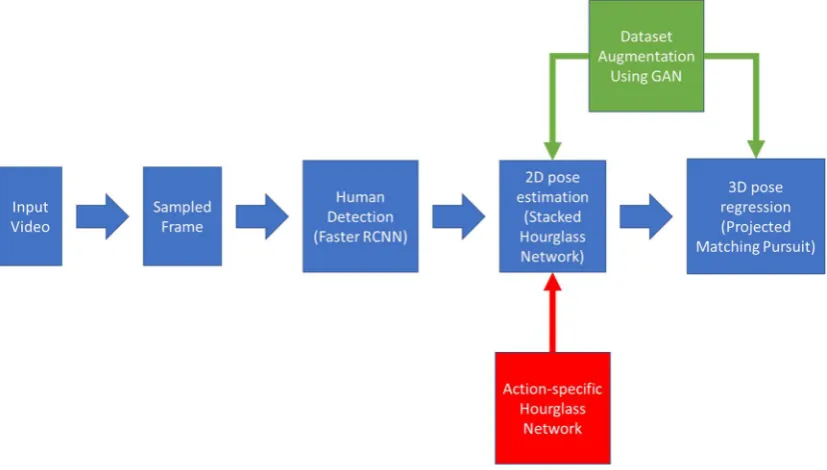
Figure 1-2: The main methods proposed/used in this thesis

Figure 1-2 shows the main methods proposed and used in this thesis as described from chapter 3 to chapter 5. The blue parts of figure 1-2 in the middle is the main 3D pose estimation pipeline detailed in chapter 3. The green part is the data augmentation method applied to different stages of the main pipeline, and it is proposed in chapter 4. The red part is the proposed action-specific hourglass network which is proposed in chapter 5.

1.4

T

HESIS CONTRIBUTIONS

The main contributions of this thesis are three-fold. Firstly, a novel three-stage CNN-based framework is proposed to estimate 3D pose of single person in RGB videos. The experiment in chapter 3 shows that this CNN-based framework can produce 3D pose estimation in RGB videos. This work is presented in the following papers:

ShangGuan, H., & Mukundan, R. (2017, December). 3D video-based motion capture using Convolutional Neural Networks. In 2017 International Conference on Image and Vision Computing New Zealand (IVCNZ) , Christchurch, 4-6 Dec 2017 (pp. 1-6). IEEE. DOI: 10.1109/IVCNZ.2017.8402458A (ShangGuan & Mukundan, 2017a)

GAN-based dataset augmentation method is proposed to solve the problem of lacking training data for unusual poses. The experiment detailed in chapter 4 shows that this GAN-based method can augment small human pose data to help the training of 3D pose estimation neural network. This work is presented in the paper:

ShangGuan, H., & Mukundan, R. (2019, June). 3D Human Pose Dataset Augmentation Using Generative Adversarial Network. In 2019 International Conference on Graphics and Signal Processing (ICGSP), Hong Kong, 1-3 June 2019 (ShangGuan & Mukundan, 2019a)

An action-specific 2D pose estimation method is developed to enhance the 2D pose estimation network by inputting action information. The experimental results presented in chapter 5 show that the proposed 2D action-specific pose estimation method can generate more accurate results.

1.5

T

HESIS ORGANIZATION

The remaining parts of this thesis are organized as follows:

this chapter. Finally, pose-guided image synthesis methods are reviewed as the basis used for the proposed dataset augmentation method in chapter 4.

Chapter 3 proposes an overall framework for 3D single human pose estimation in RGB videos based on the reviews of the related image processing areas presented in chapter 2. The three stages of the proposed pose estimation framework namely, human object detection, 2D pose estimation, and 3D pose estimation are introduced first. The methods adopted in each of the three stages are then detailed one by one. Next, a quantitative evaluation on Human3.6M dataset (Ionescu, Papava, Olaru, & Sminchisescu, 2014), and qualitative evaluation on an Olympic ice-skating video, of the three-stage method, are shown in this chapter. The merits and drawbacks of the proposed methods are discussed based on the evaluation. This proposed framework can generate 3D pose from RGB video. However, it shows defects on unusual poses. To solve this problem, data augmentation and exploitation of action information are applied and presented as two solutions.

Chapter 5 proposes an action-specific 2D pose estimation method. The proposed 2D pose estimation method tries to exploit action information for the training of 2D pose estimation neural networks. The reason why only 2D pose estimation is considered is due to a lack of 3D human pose dataset with well-annotated action information. The MPII 2D human pose dataset (M. Andriluka, Pishchulin, Gehler, & Schiele, 2014) and the containing action information are assessed first. Then two action-specific 2D pose estimation networks designed to exploit the action information of MPII datasets are presented. Next, these two designs of neural networks are evaluated using MPII datasets. The results of the experiment and comparison are presented at last. The results, however, show that action information offers limited help for the improvement of 2D pose estimation neural networks.

Chapter 6 provides the conclusion of this thesis. The main contributions of the thesis are outlined in this chapter. Also, the limitations of this research are discussed. Possible future research to extend the work and alternative solutions to remove the limitations of the research are presented.

2

Background

In this chapter, a review of previous works related to pose estimation is presented. The methods and concepts presented in this chapter are used as the basis for the main contribution of this thesis in the following chapters. Pose estimation is a sub-area of image processing. The features extracted from raw image data by image processing algorithms are used for further analysis. Section 2.1 provides an overview of some basic image-processing techniques. Section 2.2 presents the state-of-the-art pose estimation method. Section 2.3 presents an overview of pose-guided image synthesis methods.

2.1

O

VERVIEW OF SOME BASIC IMAGE PROCESSING TECHNIQUES

2.1.1

O

The most significant challenge which object detection task faces is that targets in images have a wide variation in scale, illumination, viewpoint, texture, and poses (P. F. Felzenszwalb, Girshick, McAllester, & Ramanan, 2010). A method which can detect one kind of objects may fail to detect the other kinds. Also, a method suitable for large object detection may not necessarily perform well with small object detection. For example, a region that contains an object can either cover more than 90% of the whole image or less than 10% of images, which makes methods for large objects detection fail to detect small objects.

Traditionally, an object detection method scans a large number of regions in an image. Then from each region, it extracts handcrafted features such as SIFT (Lowe, 2004), HOG (Dalal & Triggs, 2005), and Haar-like (Lienhart & Maydt, 2002) features. At last, a classifier such as SVM (Cortes & Vapnik, 1995), AdaBoost (Freund & Schapire, 1997), or DPM (P. F. Felzenszwalb et al., 2010) is applied to the extracted features to produce classification results.

Many deep learning-based object detection methods have achieved significant success. The framework of these methods can be divided into two kinds (Z. Q. Zhao, Zheng, Xu, & Wu, 2019): region proposal-based framework and the regression/classification-based framework.

2.1.1.1

R

-

Region proposal-based framework can be divided into two modules: one region proposal module for object localization and one classifier for object classification. Before the proposal of the Region-based Convolutional Network method (RCNN) (Girshick, Donahue, Darrell, & Malik, 2014a) is proposed, object detection techniques scan the whole image using a sliding window as region proposals, and the classification task has to be conducted in every sliding window. The calculation in a large number of sliding windows brings large computational loads and results in a slow process.

SPP-Net (He, Zhang, Ren, & Sun, 2015) improves the RCNN method. It only computes the CNN features once on the whole image. By applying a spatial pyramid pooling (SPP) module to normalize the scale of the extracted feature within the regional proposals, SPP-Net saves a lot of computation time. However, as in RCNN, the selective searching module used in SPP-Net is still quite slow and occupies big disk space.

Fast RCNN (Girshick, Donahue, Darrell, & Malik, 2014b) is based on SPP-Net and RCNN method. It adopts a SoftMax function for the CNN classifier and replaces the SPP module by ROI pooling module. The VGG16 convolutional network is introduced for feature extraction. It has also achieved end-to-end training by introducing multi-task losses. The fast RCNN is much faster than the original RCNN and much more accurate than SPP-Net. However, the bottleneck of Fast RCNN is still the selective searching region proposal module, which is still slow and disk-consuming.

Faster RCNN (Ren, He, Girshick, & Sun, 2017) improves the Fast RCNN method by replacing the selective searching region proposal module by a region proposal neural network. Faster RCNN firstly extracts feature maps of the whole inputted image and then uses a regional proposal neural network to regress the region proposal. Next, the regressed region proposals are cropped by a Region of Interest (ROI) pooling layer for final classification and localization. The Faster RCNN method is much faster than other previous methods. It can even be used for real-time object detection. However, due to the use of fixed scale anchor box mechanism in region proposal network, it is hard for Faster RCNN to detect small objects.

features are fed into an RPN as in Faster RCNN to regress ROI. Next features in the ROI are fed into a position-sensitive score maps network for classification. The R-FCN achieved better accuracy than Faster RCNN and is also faster than Faster RCNN. However, small object detection remains a problem.

Feature Pyramid Networks (FPN) (T. Lin et al., 2017) is developed to overcome the small object detection problem of faster RCNN. ResNet is adopted as a fundamental building block in FCN. First, a pyramid structure of feature maps with different scale is extracted. Then the features of different scale are fused for final prediction. Because information on the different scale has been kept for a final prediction, small objects are better detected by FCN.

Mask RCNN (He et al., 2018) is another extension of Faster RCNN. It replaces the RoI pooling layer by RoIAlign layer to provide scale equivariance and translation-equivariance with the regional proposals. ResNet 101 and an FPN are also used for feature extraction. Except for the object classification tasks and object localization tasks, it adds a mask generation task by adding an FCN layer after the RoIAlign layers. The FCN layer is paralleled to another two classification and localization layers.

2.1.1.2

R

/C

-

Regression/Classification-based framework uses an end-to-end one-step framework to regress object location and classification globally, unlike the two module design in the region proposal-based framework. This method is much easier to train and faster to process. The significant works of this framework include YOLO (Redmon & Farhadi, 2017) and SSD (Szegedy et al., 2015).

centroid coordinates, and a confidence score. This confidence score is a multiplication of the probability of containing an object and the Intersection over Union (IoU) between the predicted boxes and the ground truth. The design of CNN in YOLO is inspired by the GoogleNet (Szegedy et al., 2015), which is deeper and contains an inception module. The regressed bounding boxes are merged by Non-Maximum suppression method. The Yolo method is much faster than previous ones due to the simplicity of networks. However, the accuracy is lower than the other methods.

SSD method is another method applying an end-to-end CNN architecture. The input image is fed into several convolutional layers with different filter size to output several feature maps. Then these feature maps are used to predict bounding boxes by being processed by an extra feature CNN layer. Each of the boxes has the coordinates of the center, the width, the height and the probability of containing each class of object. At last, Non-Maximum suppression method is also used to merge these bounding boxes for final prediction. SSD method achieved better accuracy without lowering the process speed.

YOLOv2 (Redmon & Farhadi, 2017) is the extension of YOLO method. YOLOv2 applies many tricks to improve the performance such as batch normalization, high-resolution classifier, convolutional with anchor boxes, dimension clusters, direct location prediction, fine-grained features, and multi-scale training. These tricks significantly increase the accuracy and speed of YOLOv1.

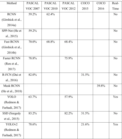
the ground truth bounding box is greater than a threshold (normally 0.5), the prediction is regarded as true prediction. In object detection, presion value 𝑝 is the fraction of true prediction over all the prediction, and it measures the accuracy of the prediction. Recall value 𝑟 is the fraction of true prediction over all the ground truth targets, and it measures how much all the positive objects have been found. Unfortunately, precision value and recall value are negatively correlated. So as a compromised metric between these two values, mAP is introduced to evaluate the performance of object detection methods. mAP is calculated as in equation 2-1.

𝑚𝐴𝑃 =∑ 𝐴𝑣𝑒𝑃(𝑞) 𝑁

𝐴𝑣𝑒𝑃 = 𝑝(𝑟)𝑑𝑟

(2-1)

Where 𝑁 is number of classes. 𝑞 is certain class. 𝐴𝑣𝑒𝑃 is average precision. 𝑟 is recall value, and 𝑝(𝑟) is presicion value at recall value 𝑟.

2.1.1

O

Object tracking is the next level of understanding images after object detection. The purpose of object tracking is to locate the target object in the consecutive input image frames, then to get the whole trajectories of the movement of the target. Usually, the location of targets at first frame will be given, and the object tracking framework needs to locate the target in the following frames.

Table 2-1: Evaluation of object detection methods

Method PASCAL VOC 2007 PASCAL VOC 2010 PASCAL VOC 2012 COCO 2015 COCO 2016 Real-Time RCNN

(Girshick et al., 2014a)

59.2% 62.4% No

SPP-Net (He et al., 2015)

59.2% No

Fast RCNN (Girshick et al.,

2014b)

70.0% 68.8% 68.4% No

Faster RCNN (Ren et al.,

2017)

78.8% 75.9% No

R-FCN (Dai et al., 2016)

82.0% 31.5% No

Mask RCNN (He et al., 2018)

39.8% No

YOLO (Redmon & Farhadi, 2017)

63.7% 57.9% Yes

SSD (Szegedy et al., 2015)

83.2% 82.2% 31.5% No

YOLOv2 (Redmon & Farhadi, 2017)

78.6% 21.6% Yes

Object tracking method faces the following challenges: deformation, illumination variation, blurry of fast motion, background clutter, out-of-plane and in-plane rotation, scale variation, occlusion, and out-of-view. These challenges make accurate and fast object tracking difficult to achieve.

performance than before in terms of both speed and accuracy. These methods can be categorized into two kinds: the generative methods and the discriminative methods. These two kinds of methods are discussed below.

2.1.1.1

G

The generative methods directly detect the moving areas from two consecutive frames, then identify the moving object, and locate the object of interest at last. So, motion detection is the first step of object tracking in this method. Generally, motion detection means extracting the changing area of image frames from the static background. For this purpose, the optical flow method is commonly adopted by the generative methods.

Optical flow is defined as the representation of the movement of objects in consecutive image frames over time caused by relative movement of objects and background. Many methods can be used to calculate optical flow. Among them, the Lucas-Kanade method (D. Lucas & Kanade, 1981) is the most popular one.

Lucas-Kanade method is based on two assumptions. One is that the object’s color does not change too much between consecutive frames. Which means:

𝐼(𝑥, 𝑦, 𝑡) = 𝐼(𝑥 + 𝛥𝑥, 𝑦 + 𝛥𝑦, 𝑡 + 𝛥𝑡) (2-2)

Where 𝐼(𝑥, 𝑦, 𝑡) is the pixel intensity of time 𝑡 at location (𝑥, 𝑦), and 𝑥 + ∆𝑥, 𝑦 + ∆𝑦, 𝑡 + ∆𝑡 are the new location and time of the moving point at the next frame.

The other assumption is that the relative movement of objects between consecutive frames is small. Based on Taylor Series, it can be represented:

𝐼(𝑥, 𝑦, 𝑡) = 𝐼(𝑥 + 𝛥𝑥, 𝑦 + 𝛥𝑦, 𝑡 + 𝛥𝑡) +𝜕𝐼 𝜕𝑥∆𝑥 +

𝜕𝐼 𝜕𝑦∆𝑦 +

𝜕𝐼

From these equations it follows that:

𝜕𝐼 𝜕𝑥∆𝑥 +

𝜕𝐼 𝜕𝑦∆𝑦 +

𝜕𝐼

𝜕𝑡∆𝑡 = 0 (2-4)

Which results in:

𝜕𝐼 𝜕𝑥𝑉 +

𝜕𝐼 𝜕𝑦𝑉 +

𝜕𝐼

𝜕𝑡= 0 (2-5)

Where 𝑉 , 𝑉 are the 𝑥 and 𝑦 components of velocity or optical flow of 𝐼(𝑥, 𝑦, 𝑡).

Thus:

𝐼 𝑉 + 𝐼 𝑉 = −𝐼 (2-6)

Which has two unknown variables, 𝑉 and 𝑉 .

Assuming that in a small window around (𝑥, 𝑦), the velocity is a fixed variable. So, at point 1, 2…n in this small window, 𝑉 and 𝑉 satisfy:

𝐼 𝑉 + 𝐼 𝑉 = −𝐼

𝐼 𝑉 + 𝐼 𝑉 = −𝐼

⋮

𝐼 𝑉 + 𝐼 𝑉 = −𝐼

(2-7)

These equations are over-determined so that they can be solved by the least squares principle as a compromise solution.

Other generative methods include mean-shift method (Comaniciu, Ramesh, & Meer, 2003), Camshift method (Bradski, 1998), Kalman filter method (Tamer, 2001) and so on. These methods build a model of the target area, based on its color or other features of the current frame and find the most similar patch in the next frame. Among these methods, the ASMS method (Vojir, Noskova, & Matas, 2013) is one of the best. It added scale estimation on the standard mean-shift framework, which can achieve 125 fps.

2.1.1.2

D

Recently the discriminative methods have outperformed the generative methods. Compared to the generative methods, the discriminative methods adopt a classic pattern which uses machine learning method to process image features. It uses the target area as a positive sample and background area as negative samples to train a classifier. Then this classifier is used to detect the target at next frame around the old location. Figure 2-1 shows the pipeline of discriminative methods.

Figure 2-1: The pipeline of the discriminative methods (Babenko, Yang, & Belongie, 2009)

discriminative methods generally perform better than the generative methods. The idea of the discriminative method is tracking by detection.

Before 2012, two classical discriminative methods of tracking by detection are TLD (Kalal, Mikolajczyk, & Matas, 2012) and Struck (Hare et al., 2016). Struck adopts Haar-like feature and structured SVM to classify an image patch into a true or false target. It also adopts an overlapping based sampling method for training. According to the Hare et al. (2016), Stuck can achieve 20 fps with 46% of mAP.

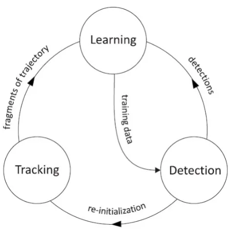
TLD is more focusing on long term object tracking. The structure of the TLD framework is shown in figure 2-2 as below. As shown in figure 2-2, TLD has three modules: tracking, learning, and detection. It combines traditional optical flow tracking method and object detection method to solve the deformation and the obstruction problem in object tracking. At the meantime, an online iterative learning mechanism is also applied to update the parameters of the tracking module and the detection module, which helps to result in a more stable, robust and reliable tracking performance. TLD can achieve 30fps and 42.5% mAP of accuracy.

which can better reflect the similarity between two images. The more features or bigger scales are introduced, the more accurate the tracking is. However, as compensation, the slower it would be.

Figure 2-2: The Framework of TLD algorithm (Kalal et al., 2012)

Generally, CF methods are much faster. However, the bottleneck of the speed of the CF methods is the strategy of the model update, and training set sampling. Model update on every frame would boost accuracy but would be slower. Sampling only on last image frame or over last several frames would also affect the performance of the application.

In recent years, deep learning methods have also been used in object tracking. GOTURN (Held, Thrun, & Savarese, 2016) method trains a deep convolutional filter on ALOV300+ (Smeulders et al., 2014) and ImageNet datasets. It is the first end-to-end deep learning-based tracking framework. It can achieve 100fps, which is comparably faster than other deep learning methods.

convolutional operator to speed up the calculation. Then a generative sample space model is proposed to maintain the diversity of samples. Also, ECO updates the model in every six frames to solve model drift problem. However, ECO can only achieve eight fps.

2.1.1.3

B

To evaluate these methods, two major benchmarks have been proposed, OTB database (Y. Wu, Lim, & Yang, 2015) and VOT database (M. Kristan et al., 2015; Matej Kristan et al., 2015; M. Kristan et al., 2013), (Matej Kristan et al., 2016). OTB (Object Tracking Benchmark) has 100 more videos, mostly small videos. VOT (Visual Object Tracking) are challenges in object tracking area held every two years. There are three significant differences between these two benchmarks:

 All the videos in VOT are color videos, but in OTB quarter of videos are grey scale videos. Also, VOT videos have higher resolution. It results in the different performance of color-based tracking methods on these two benchmarks.

 In VOT challenge, the tracking initializes at the first frame. Whereas in OTB, it starts at a random frame.

 VOT focuses on short-term tracking, and OTB focuses on long-term tracking. Short term tracking tolerates model drifting, but long term tracking does not.

2.1.2

A

learning algorithm in object detection and tracking, the task of activity recognition remains an unsolved problem due to the following challenges:

1. The diversity of representation of activity: activity recognition task involves capture spatiotemporal feature and context throughout multiple frames. The same activity can be shown differently due to the different environment setting such as lighting, obstruction, resolution, camera viewpoint, background, or different people who perform in a different style. With the same activity, the feature extracted from the videos can be different. Additionally, in a video, the beginning and the end of action are hard to be identified. All of the challenges above affect the activity recognition of a video.

2. Huge computation cost: compared to simple 2D image processing, the multi-frame video feature extraction requires 3D convolution networks for activity recognition problems which contain much more trainable parameters, and takes much longer time to train.

happens, which is hard to go through for training. New datasets called Kinetics-600 (Kay et al., 2017) and Moments in Time (Monfort et al., 2019) are released. Kinetics-600 contains a massive scale of well-annotated video clips of more than 600 types of activities, and every type of activity is contained in more than 600 video clips. Moments in Time dataset contains one million 3 seconds labeled video clips. Compared with other datasets, Moments in Time dataset is more focused on different actions rather than the different context of actions. These new datasets show the potential to solve the problem of lack of benchmark.

To overcome these challenges, many methods have been developed. Traditionally, the activity recognition task is divided into three major steps (Dollár, Rabaud, Cottrell, & Belongie, 2005; Laptev, 2005; Wang, Kläser, Schmid, & Cheng-Lin, 2011; Wang & Schmid, 2013):

1. Local high-dimensional features are extracted to describe a local region in a video.

2. These locally extracted features are combined to encode video-level features. 3. A classifier is trained to classify the combined features into the final prediction.

After convolutional neural network is introduced to extract features and classify for prediction, the activity recognition CNN can be divided into two categories: single stream networks and two steam networks.

For single stream networks, only the spatial information of frames is used to infer the classifications of activities. The ground-breaking research of these methods is the work (Karpathy et al., 2014). According to this work (Karpathy et al., 2014), Karpathy et al. tried multiple strategies to fuse the extracted features for further prediction, as shown in figure 2-3.

In figure 2-3, red, green and blue boxes indicate convolutional, normalization and pooling layers respectively. In slow fusion, the parallel layers share weights.

Figure 2-3: Different strategies to fuse features (Karpathy et al., 2014)

first stage. Slow fusion architecture adopts a multi-stage fusion architecture, which is a balance between early fusion and late fusion.

In single stream networks, only spatial information of one frame is captured in most networks, which ignores temporal information. Hence, each of the explored strategies above shows much worse performance than the iDT method which uses the handcrafted spatiotemporal feature.

For two stream method, based on the failure of previous works, optical flow is introduced to capture the motion features of videos. So, network architecture in this method has two separated parts, one for the spatial feature extraction and the other for temporal feature extraction. The spatial context network takes only a single frame of the video as input, and the temporal network takes pre-calculated optical flow as input. The optical flow contains information from multiple frames. The two networks are trained separately. Then the extracted features are combined at the following stage to train a classifier like SVM for prediction. This method is proposed by Simmoyan and Zisserman (Simonyan & Zisserman, 2014a). Though it has achieved better performance than single stream method, it still has many drawbacks such as missing long-range temporal information, false label assignment, and considerable pre-computation effort for optical flow.

Figure 2-4: Summarization of recent activity recognition method (Carreira & Zisserman, 2017)

To capture long-term motion information throughout videos, the long short-term memory networks (LSTMs) which are capable of learning long-term dependencies seem a natural option. Long-term recurrent convolutional network (LRCN) is developed by Donahue (Donahue et al., 2015) for video visual recognition and description. It adopts LSTM to encode the computed spatial information for the following prediction. In this work, different input choices including RGB input, weighted RGB and optical flow input are tested and compared. This method proposes an end-to-end trainable framework. The result of this work shows that it is still hard to avoid missing of long-range temporal information and pre-calculation of optical flow.

networks to combine the extracted features across consecutive frames, which has achieved better results.

Feichtenhofer et al. (Feichtenhofer, Pinz, & Zisserman, 2016) have developed a novel TSN method which takes a two-steps fusion strategy. At the first step, temporal feature and spatial feature are fused as same as previous methods. Then at the second step, after several layers of processing, the post-processed spatial feature will be fused again with the post-processed spatiotemporal feature for final prediction. This method improves the performance of C3D without increasing the number of parameters by applying a soft-attention technique.

TSN (L. Wang et al., 2018) method also adopts the two-stream architecture. The contribution of TSN is that it proposes a sparsely sampling strategy and explores the usage of batch normalization and dropout techniques for long term temporal information extraction. Other evolutions of TSN adopt different fusion techniques (Lan, Zhu, Hauptmann, & Newsam, 2017; B. Zhou, Andonian, Oliva, & Torralba, 2017).

updating. This method can successfully transfer the knowledge from 2D pre-trained networks to the T3D networks.

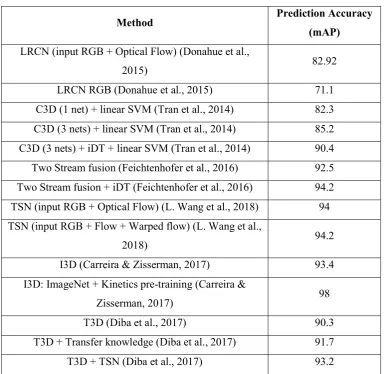
Table 2-2: The performance of methods on UCF101 dataset

Method Prediction Accuracy

(mAP)

LRCN (input RGB + Optical Flow) (Donahue et al.,

2015) 82.92

LRCN RGB (Donahue et al., 2015) 71.1 C3D (1 net) + linear SVM (Tran et al., 2014) 82.3 C3D (3 nets) + linear SVM (Tran et al., 2014) 85.2 C3D (3 nets) + iDT + linear SVM (Tran et al., 2014) 90.4

Two Stream fusion (Feichtenhofer et al., 2016) 92.5 Two Stream fusion + iDT (Feichtenhofer et al., 2016) 94.2 TSN (input RGB + Optical Flow) (L. Wang et al., 2018) 94 TSN (input RGB + Flow + Warped flow) (L. Wang et al.,

2018) 94.2

I3D (Carreira & Zisserman, 2017) 93.4 I3D: ImageNet + Kinetics pre-training (Carreira &

Zisserman, 2017) 98

T3D (Diba et al., 2017) 90.3

T3D + Transfer knowledge (Diba et al., 2017) 91.7 T3D + TSN (Diba et al., 2017) 93.2

2.2

P

OSE ESTIMATION

Pose estimation in computer vision area is a task to locate humans’ key joints in single-view images or videos. As shown in Figure 2-5, by locating these key joints, a human’s skeletal information can be appropriately described so that this information can be further used for another computer vision tasks like activity recognition, human object tracking, human animation. The key joints being estimated usually include: head, neck, wrist, shoulders, elbows, knees, ankles, and hips.

Figure 2-5: Representation of human pose, by locating key joints (Bearman & Dong, 2015)

Pose estimation faces several challenges:

 The variety of human poses: human body is soft, flexible and diverse. A human can play a wide variety of poses. Every joint of the human body has six degrees of freedom. Different poses played by same people present an entirely different appearance. Also, when different people play the same pose, they can result in different presentation due to the differences in height, weight or other conditions.

can tackle one kind of environment setting would not be suitable for another one. Additionally, in many images, parts of a human body are obstructed. So, it is even harder to estimate these joints.

 A lack of benchmarks: Annotating images for pose estimation takes a considerable effort. Years before, most pose estimation datasets were created in a laboratory setting, which means that they lack the complexity of the environmental settings. 2D pose estimation benchmark like LSP and MPII dataset contains the massive scale of images in the wild. However, most 3D human pose benchmarks contain images produced in a laboratory, which makes 3D human pose estimation area progresses much slower.

2.2.1

B

Table 2-3: The Comparison of Human Pose datasets

dataset numbers of samples number of joints

Posetrack (Mykhaylo Andriluka et al., 2017) 20K 17 LSP (Johnson & Everingham, 2010) 2K 14

FLIC (Sapp & Taskar, 2013) 20K 9

MPII (M. Andriluka et al., 2014) 25K 16

MSCOCO (T.-Y. Lin et al., 2014) 300K 18

AI challenger (J. Wu et al., 2017) 270K 14

For evaluation of pose estimation method, many human pose benchmarks have been created. Some information on 2D human pose benchmarks is listed as table 2-3.

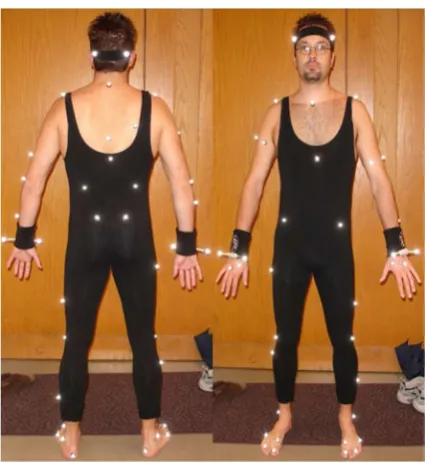
Figure 2-6: The laboratory setting of poses recording in 3D human pose datasets (CMU, 2011)

For 3D pose estimation, it is difficult to collect 3D human pose information in an outdoor or natural environment. So, almost all of the 3D human pose data sets are collected in laboratory settings such as HumanEva (Sigal, Balan, & Black, 2009), Human3.6m (Ionescu et al., 2014), MPI-INF-3DHP (Mehta et al., 2016), and CMU Mocap Dataset (CMU, 2011). All of the pose data in these datasets are recorded by Motion capture sensors wearing at the body of subjects in a laboratory setting, as shown in figure 2-6.

Because all of these datasets are recorded in a laboratory setting, these data cannot represent human poses in real life scenarios. A pose estimation method which can tackle some of the datasets is not necessarily suitable for pose estimation in the wild. Another problem of these datasets is that there are a lack of unusual poses such as skating or gymnastics, which would result in many incompatible issues of the pose estimation methods.

DensePose (Alp Güler, Neverova, & Kokkinos, 2018) focuses on the UV prediction of 3D Human body. It created a database called COCO-Densepose-dataset based on MSCOCO database. This COCO-Densepose-dataset has images with UV coordinates of 50K people. Also, human part segmentation is included. This database allows CNN to predict UV coordinates of the 3D human body so that better texture mapping is possible for the future CNN-based pose estimation methods.

2.2.2

O

Figure 2-7: Pictorial Structures (Pedro F. Felzenszwalb & Huttenlocher, 2005)

This kind of method cannot cover the diversity and complexity of human poses. When machine learning is introduced into pose estimation area, it has been the universal method of design. Below is a review of machine learning based pose estimation methods.

2.2.2.1

S

2D

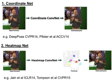
Figure 2-8: The difference between Coordinates Net and Heatmap Net (Tompson et al., 2014;

Toshev & Szegedy, 2014)

Figure 2-9: Architecture and receptive fields of CPM (Wei, Ramakrishna, Kanade, & Sheikh,

2016)

Stack Hourglass network adopts a classical encoder-decoder architecture as shown in figure 2-10. It uses residual modules to keep the original information through the layers, which enables to better capture features from multi-scale resolutions. Like in CPM, intermediate supervision in every stage is conducted to avoid the vanishing gradient problem. Stack hourglass network has achieved much higher accuracy than previous methods, and also processes significantly faster than CPM. Since it has been proposed, the single-person pose estimation methods mostly adopt the stack hourglass architecture, such as Structured Feature Learning (Chu, Ouyang, Li, & Wang, 2016), Adversarial Posenet (Y. Chen, Shen, Wei, Liu, & Yang, 2017) and CPF (Hong Zhang et al., 2019).

2.2.2.2

M

-

2D

Multi-person 2D pose estimation tackles images with more than two people. It needs to not only locate the key joints in the image but also find out which key joint belongs to which person. There are two kinds of methods for this problem: top-down approaches and bottom-up approaches.

Top-down approaches break down the multi-person pose estimation task into two sub-tasks. Firstly, it detects all the people in the image and locates them by object detection method. Secondly, to every detected person, it applies single-person pose estimation for final prediction. This kind of approaches includes RMPE (Fang, Xie, Tai, & Lu, 2017), Mask RCNN (He et al., 2018), G-RMI (G. Papandreou et al., 2017), Cascaded Pyramid (Y. Chen et al., 2018) and so on. The drawback of these approaches is that false human detection will affect the accuracy of the final pose result.

Hidalgo, Simon, Wei, & Sheikh, 2018; Z. Cao, Simon, Wei, & Sheikh, 2017; Simon, Joo, Matthews, & Sheikh, 2017), DeepCut (Z. Cao et al., 2017; Simon et al., 2017), ArtTrack (Eldar Insafutdinov, Pishchulin, Andres, Andriluka, & Schiele, 2016; Pishchulin et al., 2016), Associative Embedding (Newell, Huang, & Deng, 2017), and Mid-Range Offsets (George Papandreou et al., 2018) all belong to this kind of approaches. The drawback of these approaches is that it will result in false estimation of correlation of joints.

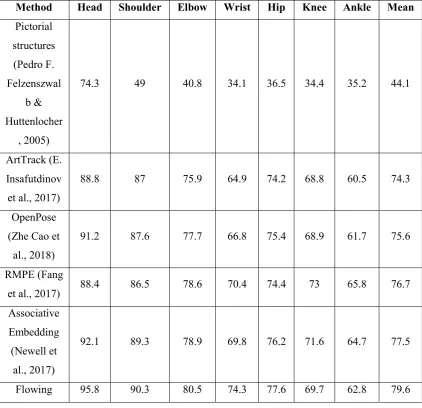
Some of the results of the mentioned methods above are shown below in table 2-4. In the MPII database, PCKh0.5 is metric of PCK setting when the threshold is 50% of the head bone link.

Table 2-4: PCKh0.5 index of pose estimation method in MPII datasets

Method Head Shoulder Elbow Wrist Hip Knee Ankle Mean

Pictorial structures (Pedro F. Felzenszwal b & Huttenlocher , 2005)

74.3 49 40.8 34.1 36.5 34.4 35.2 44.1

ArtTrack (E. Insafutdinov et al., 2017)

88.8 87 75.9 64.9 74.2 68.8 60.5 74.3

OpenPose (Zhe Cao et

al., 2018)

91.2 87.6 77.7 66.8 75.4 68.9 61.7 75.6

RMPE (Fang

et al., 2017) 88.4 86.5 78.6 70.4 74.4 73 65.8 76.7 Associative

Embedding (Newell et

al., 2017)

92.1 89.3 78.9 69.8 76.2 71.6 64.7 77.5

Convnets (Tompson et

al., 2014). Deepcut (Pishchulin et al., 2016)

94.1 90.2 83.4 77.3 82.6 75.7 68.6 82.4

Deepercut (Eldar Insafutdinov

et al., 2016)

96.8 95.2 89.3 84.4 88.4 83.4 78 88.5

CPM (Wei et

al., 2016) 97.8 95 88.7 84 88.4 82.8 79.4 88.5 Stacked

Hourglass (Newell et al., 2016)

98.2 96.3 91.2 87.1 90.1 87.4 83.6 90.9

Adversarial Posenet (Y. Chen et al.,

2017)

98.1 96.5 92.5 88.5 90.2 89.6 86 91.9

CPF (Hong Zhang et al.,

2019)

98.6 97 92.8 88.8 91.7 89.8 86.6 92.5

2.2.2.3

3D

In terms of 3D pose estimation, there are two types of approaches: two-stage approaches and one stage approaches.

work developed by Marinez et al. in 2017 (Martinez, Hossain, Romero, & Little, 2017). In this work, the framework is shown in figure 2-11.

Figure 2-11: The framework in Two-stage approaches (Martinez et al., 2017)

As shown in figure 2-11, The 2D pose estimation module is trained both by 3D data from Human3.6M datasets, and other 2D pose datasets. The 3D depth regression module is trained by 3D pose data solely. This design enables the model to transfer restriction-free data from the wild for 3D pose estimation.

Figure 2-12: The multi-source discriminator (Yang et al., 2018)

Coarse-to-Fine volumetric prediction (G. Pavlakos, Zhou, Derpanis, & Daniilidis, 2017) is another two-stage approach. It adopts 3D volumetric representation for the human pose. For each joint, it discretizes the space around the subject and uses a convolutional network to regress per voxel likelihood. A significant advantage of the volumetric representation is that it casts the highly non-linear problem of direct 3D coordinate regression to a more manageable form of prediction in a discretized space. A Coase-to-fine strategy is also used in this method.

One stage approaches (Vosoughi & Amer, 2018)regress 3D poses regression directly from an image. For example, VNect (Mehta et al., 2017) is developed to tackle real-time 3D human pose estimation from mono-view images by applying deep ResNet (He, Zhang, Ren, & Sun, 2016) for human pose regression. All of this kind of methods require a large number of labeled training data to train the CNN properly. The method (Mehta et al., 2018) is an extension of VNect by introducing an Occlusion-Robust Location Maps (ORLM) that make VNect robust for partial occlusions of the human body.

Recently, SMPL-based (Loper, Mahmood, Romero, Pons-Moll, & Black, 2015) method is developed to enable full shape estimation. The SMPL model allows human body model to be decomposed into pose and shape parameters, so it can be used to sample parameters to produce human body model and images. It also can be used to match the shape from an image. Georgios et al. (2018) ’s method is one of them which allows end-to-end estimation of 3D pose from a single RGB image (Omran, Lassner, Pons-Moll, Gehler, & Schiele, 2018; Georgios Pavlakos et al., 2018). Georgios et al. (2018) ’s method also adopts two-stage approaches. At the first stage, it trains a convolutional neural network to output a heatmap for 2D pose estimation and also to output a mask of the human body which is supervised by pixel-wise binary cross entropy loss. Then at the second stage, a poseprior and shapeprior are trained. The poseprior is applied to regress 72 pose parameters of SMPL model from 2D key point estimation result, and the shapeprior is used to estimate the shape parameters of the SMPL model from a 2D mask. The training data used here are generated by sampling from the SMPL model.

key point loss. These three training tasks all lead to better accuracy in 3D pose estimation and shape estimation. The SMPL model is also used in this method for evaluation. Another shape estimation method (Xu et al., 2018) is developed by using silhouette-based pose refinement method to improve the 3D pose estimation and shape estimation.

For 3D pose estimation in video, Detect-and-Track method (Girdhar, Gkioxari, Torresani, Paluri, & Tran, 2018) is proposed to estimate 3D poses from videos by adopting 3D Mask R-CNN. 3D Mask R-CNN is an extension of 2D Mask R-CNN (He, Gkioxari, Dollár, & Girshick, 2017). It replaces the 2D convolutional layers in Mask R-CNN by 3D convolutional layers to process videos. So the RPN in 2D Mask R-CNN becomes 3D tube proposal network (TPN) to detect spatiotemporal proposal tubes. Then these tubes are used to extract 3D features by RoIAlign method. These features are fed into a classifier network to determinate its categories and also fed into a pose estimation network to regress joints positions in every frame of a video. The joints positions in every frame are linked by a deep recurrent neural network (RNN) as introduced in object tracking in section 2.1.2. So the Detect-and-Track method can decide which joints belong to which person. This method has achieved success in PoseTrack database (Mykhaylo Andriluka et al., 2017). Based on Detect-and-Track method, several methods (Pavllo, Feichtenhofer, Grangier, & Auli, 2018; F. Zhou & De la Torre, 2016) are also proposed to use temporal convolutions.

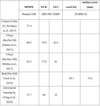
Evaluation of the mentioned methods on different datasets is shown in table 2-5. The results shown in table 2-5 are all taken from the original paper.

The accuracy of 2D and 3D pose estimation task can be evaluated by the mean of per joint position errors (MPJPE), which is the Euclidean distance of the estimated joints positions to the ground truth (ShangGuan & Mukundan, 2017a). Another metric for evaluation of pose estimation is Percentage of Correct Keypoints (PCK) which represents the percentage of pose estimation that falls within a normalized distance of the ground truth.

Table 2-5: Evaluation of the 3D pose estimation methods

MPJPE PCK AUC voxel IoU

surface error (mm)

Human3.6M MPI-INF-3DHP SURREAL

Coarse-to-fine (G. Pavlakos

et al., 2017)

71.9

VNect (ResNet 50) (Mehta et al.,

2017)

80.5 79.4 41.6

VNect (ResNet 100) (Mehta et al.,

2017)

82.5 77.8 41

BodyNet (Gül Varol et al.,

2018)

58.1 73.6

Adversarial learning by (Yang et al.,

2018)

simple effect (Martinez et

al., 2017)

52.1

2.3

P

OSE

-

GUIDED IMAGE SYNTHESIS

As recent human pose estimation methods are mostly based on convolutional neural network, which needs a large amount of well-annotated images for training. Hence one of the bottlenecks of CNN based pose estimation method is a lack of training data. Pose-guided image synthesis method can create images that contain a person performing a given human pose. It can be used for video synthesis. It also can be used to augment datasets for the training of human pose estimation neural networks.

There two kinds of pose-guided image synthesis method. One of them is to use a 3D mesh model to animate 3D sequences of motion capture data. The idea is that it can randomly assign poses to mesh models and then easily record them.

Surreal datasets (G. Varol et al., 2017) are built on ground truth pose data from Human3.6m dataset. It contains 6 million frames of photo-realistic renderings of people. The shape, texture, viewpoint, and pose are variated in this dataset. The human mesh model used in SURREAL is SMPL body model. Given raw 3D mocap pose data, it can fit realistic human mesh using Mosh method (Loper, Mahmood, & Black, 2014). The SURREAL dataset contains the massive scale of the ground truth of depth, body part, optical flow, 2D/3D pose and surface normal.

all 30 seconds long, recorded at 30 fps. These videos are recorded in a photorealistic video game which is Grand Theft Auto V developed by Rockstar North.

Another method for pose-guided image synthesis is using neural network-based methods such as Variational Autoencoders (VAE) (Kingma & Welling, 2013), Generative Adversarial Networks (GAN) (Goodfellow et al., 2014) and Autoregressive models (e.g., PixelRNN (Oord, Kalchbrenner, & Kavukcuoglu, 2016)). Recently, GAN based methods achieved popularity in image synthesis areas by their excessive ability to generate photorealistic images through adversarial training. Hence, it shows potential to generate images for the training of pose estimation method.

2.3.1

GAN

2.3.1.1

I

GAN

Generative adversarial network now is the most popular image synthesis method in the image processing area. This kind of network adopts a creative adversarial two-module architecture, one generator 𝐺 to synthesize images, and one discriminator 𝐷 to evaluate the quality of the synthesized images.

Figure 2-13: The Generator of GAN (Hui, 2018)

The discriminator 𝐷 provides guidance for generator 𝐺 to synthesize the target kind of images. Without discriminator 𝐷, the generator will output random noises. The discriminator is a binary classifier. The standard training process of GAN is shown in Figure 2-14.

Figure 2-14: The training process of GAN

1. Mode collapse: the generator fails to output wide varieties of images. Partial collapse happens often. As shown in figure 2-15, many of output images are very similar.

Figure 2-15: Mode Collapse of GAN (Berthelot, Schumm, & Metz, 2017)

2. Gradient vanishing: sometimes, the discriminator is trained much better than the generator, which makes the gradient of the generator vanish. So the generator stops learning.

3. Non-convergence: the model never converges when the parameters oscillate. It is most likely caused by unbalanced training between a discriminator and a generator.

4. Unknown hyperparameters: GAN is sensitive to the setting of hyperparameters. Sometimes, GAN can only perform well with a short range of hyperparameters setting. Tuning these hyperparameters are not easy.

2.3.1.2

T

GAN

The GAN has been researched for years. Many varieties of GAN have been proposed to improve the performance of GAN. These varieties mainly focused on two aspects of GAN: network design and cost function.

 Network design

DCGAN (Heusel et al., 2017) is one of the most popular GAN network designs. The architecture of the DCGAN is shown in figure 2-16. The main idea of DCGAN is to apply a convolutional neural network to better the performance of GAN. It uses convolutional stride layer to replace the max pooling layer in original GAN. The transposed convolutional layer which replaces the fully-connected layer is also applied for upsampling. Additionally, Batch normalization is applied in DCGAN.

Figure 2-16: The architecture of DCGAN (Radford, Metz, & Chintala, 2015)