Spatial correlation of two dimensional Bosonic multimode condensates

Spatial correlation of two-dimensional bosonic multimode condensates

Wolfgang H. Nitsche,1,*Na Young Kim,1,†Georgios Roumpos,1,‡Christian Schneider,2Sven H¨ofling,2,3,4 Alfred Forchel,2_{and Yoshihisa Yamamoto}1,4

1_{E. L. Ginzton Laboratory, Stanford University, Stanford, California 94305, USA} 2_{Technische Physik, Universit¨at W¨urzburg, Am Hubland, 97074 W¨urzburg, Germany} 3_{School of Physics & Astronomy, University of St Andrews, St Andrews KY16 9SS, United Kingdom}

4_{National Institute of Informatics, Hitosubashi, Chiyoda-ku, Tokyo 101-8430, Japan}

(Received 10 October 2015; published 23 May 2016)

The Berezinskii-Kosterlitz-Thouless (BKT) theorem predicts that two-dimensional bosonic condensates exhibit quasi-long-range order which is characterized by a slow decay of the spatial coherence. However previous measurements on exciton-polariton condensates revealed that their spatial coherence can decay faster than allowed under the BKT theory, and different theoretical explanations have already been proposed. Through theoretical and experimental study of exciton-polariton condensates, we show that the fast decay of the coherence can be explained through the simultaneous presence of multiple modes in the condensate.

DOI:10.1103/PhysRevA.93.053622

I. INTRODUCTION

Two-dimensional bosonic systems at low temperatures have been observed to exhibit spatial coherence over long distances [1–5]. Although Bose-Einstein condensation with true long-range order is not possible in such systems [6,7], they can still exhibit quasi-long-range order by condensing into a state which is described by the Berezinskii-Kosterlitz-Thouless (BKT) theory [8,9]. In this case, the first-order spatial correlation function is predicted to decay with a power law (algebraically), whose exponent must always be1/4 [5,10]. Previous studies [5] however observed that the measured coherence of an exciton-polariton condensate typically decays much faster than allowed by the BKT theory and tried to explain this through noise caused by the continuous generation and decay of exciton-polaritons. Here, we show through theoretical and experimental studies of an exciton-polariton condensate that the fast decay of the spatial coherence can be explained through simultaneous condensation into several spatioenergetic modes. The Nozi`eres principle [11] in general predicts that condensation will only occur into a single mode since condensate fragmentation is energetically costly due to the Fock exchange term; however multimode condensation is possible in the studied exciton-polariton system where the energy uncertainty caused by the short boson lifetime is greater than the Fock exchange energy.

*_{Corresponding author. Present address: Halliburton, Houston,}

Texas 77032.http://www.nitsche.mobi; [email protected] †_{Present address: University of Waterloo, 200 University Avenue} West, Waterloo, Ontario N2L 3G1, Canada.

‡_{Present address: Google, Mountain View, California 94043.} Published by the American Physical Society under the terms of the

Creative Commons Attribution 3.0 License. Further distribution of this work must maintain attribution to the author(s) and the published article’s title, journal citation, and DOI.

II. BOSONIC CONDENSATE WITH CONSTANT DENSITY

We study a finite-sized two-dimensional bosonic con-densate with a nearly constant particle density n_total(x,y) throughout the condensate. In this paper, we focus on the case,

ntotal(x,y)≈nconstH(Rspot−

x2+_y2_),

whereH is the Heaviside step function. This corresponds to the most relevant case of a condensate occupying a circular area with radius Rspot; but condensates with rectangular or

other forms could be studied in an analog way. Such a condensate with a constant density cannot be in a single quantum-mechanical mode since this would require a wave function whose amplitude is constant within the circular area and zero everywhere else, but such a wave function is not an eigenfunction to the Schr¨odinger equation. However a nearly constant total density is possible if condensation occurs simultaneously into several spatioenergetic modes s which

gives1a total wave function of the form

total(x,y,t)=

s

s(x,y,t), (1)

where a mode numbersis described by

s(x,y,t)=Asψs(x,y)e−itEs/eiηs(x,y,t). (2)

Due to the circular symmetry of the condensate, each base-function ψs can be expressed [12] (in polar coordinates) as

ψs(r,φ)=Jm_s(ksr) exp(imsφ)H(Rspot−r), (3)

where the orbital quantum numberms is an integer,J is the

Bessel function of the first kind, the positive ks is chosen so

that the Bessel function reaches one of its zeros atr=Rspot,

andEs is the energy corresponding to base-functionψs. The

amplitudesAsare determined by the condition,

total(x,y,t)total† (x,y,t) =ntotal(x,y). (4)

1_{Here, we assume a condensation fraction of nearly 100%; if we}

The realηs(x,y,t) represents phase noise and can, for

ex-ample, be explained by the thermal excitation [10] of phononic long-wavelength phase fluctuations. Without this phase noise, coherence could exist over arbitrary long distances which is not possible [6,7] in our two-dimensional system. The· · · brackets indicate time averaging.

III. CORRELATION FUNCTION OF OUR SYSTEM

The first-order spatial correlation function can be defined as

g(1)(x1,y1,x2,y2)=

|(x1,y1,t)†(x2,y2,t)|

|(x₁,y₁,t)|2_|(x

2,y2,t)|2

, (5)

and it reaches a value of 1 if there is perfect coherence between points (x₁,y₁) and (x₂,y₂), but its value is 0 if there is no coherence between these points. The coherence for each individual modescan therefore be written as

g_s(1)(x1,y1,x2,y2)= |

s(x1,y1,t)s†(x2,y2,t)|

|s(x1,y1,t)|2|s(x2,y2,t)|2

= |exp{i[η(x1,y1,t)−η(x2,y2,t)]}|. (6)

It can be shown [10] that for condensation into a single-modes, this coherence function over long distances behaves

like

g(1)_s (x₁,y₁,x₂,y₂)∝

(x₁−x₂)2+(y₁−y₂)2 ₋ap

, (7)

withap 1/4. For short distances, the coherence function is

expected to converge towards 1. The coherence of the total systemtotalcan be calculated [using Eqs. (1), (2), and (6)] as

g(1)_total(x1,y1,x2,y2)

= |total(x1,y1,t)total† (x2,y2,t)|

|_total(x₁,y₁,t)|2|_total(x₂,y₂,t)|2

= s|As|2ψs(x1,y1)ψs†(x2,y2)g(1)s (x1,y1,x2,y2)

s|Asψs(x1,y1)|2 s|Asψs(x2,y2)|2

. (8)

Here we used

expiηs1(x1,y1,t)−ηs2(x2,y2,t)

exp

−iEs1−Es2

t

=expiηs1(x1,y1,t)−ηs2(x2,y2,t)

δ(s1,s2), (9)

which assumes that the energies are nondegenerate so that fors1=s2all interference terms with exp[−i(Es1−Es2)t /]

-100 -5 0 5 10

0.5 1

x( m)

g

(1

)(x

,-x

)

0 5 10

0 0.5 1

r( m)

D

e

n

s

it

y

(a

.u

.)

n_wanted I_pump

n

total = s|As s|

2

|A

4 4| 2

= |1.95e-0.54428 iJ 2(0.5136r)|

2

|A_{5 5}|2 = |0.46e-2.31 iJ_-2(0.5136r)|2

|A_{7 7}|2 = |0.72e1.7499 iJ₁(0.7016r)|2

|A_{8 8}|2 = |1.45e-2.847 iJ_-1(0.7016r)|2

|A

9 9| 2

= |1.03e-0.26699 iJ 0(0.8654r)|

2

x( m)

y

(

m)

-10 -5 0 5 10

-10

-5

0

5

10

0 0.5 1

x( m)

y

(

m)

-10 -5 0 5 10

-10

-5

0

5

10

0 1 2 3 4

x( m)

y

(

m)

-10 -5 0 5 10

-10

-5

0

5

10

0 0.5 1

x( m)

y

(

m)

-10 -5 0 5 10

-10

-5

0

5

10

-3.14 0 3.14

(c) (b)

(a)

(d) (e) (f)

FIG. 1. Simulated data. (a) A total densityntotal(r) compared to thenwanted(r)=H(10μm−r)×1a.u. The contributions|Ass(r,φ)|2

of the individual modes are also shown. (b) A total densityntotal(x,y). (c) The interference signal as it would be measured by the camera

of a Michelson interference setup. (d) The phase as it would be determined through evaluating interference data. (e) A correlation function

gtotal(1) (x,y,−x,y) as it would be calculated from the interference data. (f) All the values of (e) but plotted as a function ofx. Each gray point

-100 -5 0 5 10 0.5

1

x( m)

g

(1

)(x

,-x

)

-100 -5 0 5 10

0.5 1

x( m)

g

(1

)(x

,-x

)

-100 -5 0 5 10

0.5 1

x( m)

g

(1

)(x

,-x

)

x( m)

y

(

m)

-10 -5 0 5 10 -10

-5

0

5

10

0 0.5 1

x( m)

y

(

m)

-10 -5 0 5 10 -10

-5

0

5

10

-3.14 0 3.14

x( m)

y

(

m)

-10 -5 0 5 10 -10

-5

0

5

10

0 0.5 1 x( m)

y

(

m)

-10 -5 0 5 10 -10

-5

0

5

10

-3.14 0 3.14

x( m)

y

(

m)

-10 -5 0 5 10 -10

-5

0

5

10

0 0.5 1 (e)

(d)

(c)

(f) (a) (b)

(g) (h) (i)

x( m)

y

(

m)

-10 -5 0 5 10 -10

-5

0

5

10

-3.14 0 3.14

FIG. 2. Measured data. (a)–(c) Measured phase (a) and visibility (b) and (c) of an exciton-polariton condensate with nearly constant density which has been created by pumping the sample with a top-hat profile at low temperature (≈7K). The decay of the visibility is significantly faster than measured (i) for a single-mode BKT condensate [4] with quasi-long-range order. Pseudovortices which appear as forks in (a) are clearly visible. Each gray point in (c) corresponds to one pixel of (b), and the continuous black line in (c) has been calculated by averaging all the gray data points with the samexvalue. (d)–(f) The same kind of measurement (still with a top-hat pump profile) at≈200K where the coherence can only be explained by VCSEL lasing. Nevertheless, the behavior is the same as for (a)–(c), which confirms that the visibility is determined by the presence of several quantized modes rather than by the intrinsic coherence properties of a condensate. (g)–(i) The same kind of measurement at low temperatures (≈5K) with a Gaussian pump profile which excites a single-mode exciton-polariton condensate. No pseudovortices (forks) appear in the phase map (g).

average out to zero.2 _{Equation (8) shows that even if each}

individual mode is perfectly coherent (g(1)_s ≈1), the overall coherenceg_total(1) can nevertheless exhibit a fast decay as a direct result of the simultaneous excitation of several modess. The

details of which modess are excited are determined by the

spatial particle densityn_total(x,y) with which the condensate is created. This also implies that if we create a condensate having a (nonconstant) particle densityntotal(x,y)= |s˜(x,y)|2which

comprises only one chosen modes˜, we getAs =0 fors=s˜,

2_{If the camera which records the interference image has an}

integration time of t=1s, this assumption will be true as long as the energy difference between different states is larger thanE= h/t≈6.63×10−34_J=4.14×10−15_{eV. Even for two modes as}

defined in Eq. (3) which differ only by the sign ofms, under real

experimental conditions there will always be a sufficient symmetry breaking which causes an energy difference of more than thisE.

butAs_˜ =0, and the coherenceg_total(1) becomes identical to the

coherenceg_s(1)_˜ of the chosen mode.

IV. MICHELSON INTERFEROMETER

The correlation function and phase of a condensate could, for example, be determined with a Michelson interferometer which flips the signal in one arm around the y axis so that effectivelytotal(x,y) interferes withtotal(−x,y) as explained

in previous papers [4,5]. The measured intensity (as a function of the path-length difference L between both arms of the Michelson interferometer),

I_measured=IB+IAsin (w L−ϕ0) (10)

tells us the phaseϕ0 and the visibilityg(1)=IA/IB for each

point. The average intensityIB is approximately proportional

to temporal coherence and similar aspects do not affect the measurement.

V. SIMULATED DATA

For the simulation, we choose a few possible modessand

fit the amplitudesAsso thatntotal(x,y) is approximately

pro-portional toH(10μm−x2_+y2_{) as shown in Figs.1(a)and} 1(b). The intensity [Fig.1(c)] of the Michelson interference image as it would be measured is

I_interference(x,y)∝ |_total(x,y,t)+_total(−x,y,t)eiα(x)|2

=

s

|As|2{|ψs(x,y)|2+ |ψs(−x,y)|2

+2g_s(1)(x,y,−x,y) × [ψs(x,y)ψs†(−x,y)e−

iα(x)_{]}, (11)}

where the phase differenceα(x)≈w L+vxis determined by the path-length differenceLand the different angle with which the signals from both arms reach the plane where the intensity is measured.3_{Even with the assumption ofg}(1)

s ≈1

(which we used for the simulations since the predicted slow algebraic decay is negligible over the small condensate size), theg(1)_total(x,y,−x,y) which we simulated using Eq. (8) shows a clear decay [Fig. 1(f)]. The simulated interference signal [Fig. 1(c)] and the simulated interference phase [Fig. 1(d)] show forks in the fringes which look similar to trapped vortices [13], but in our case, where we did not assume any trapped vortices, they are an artifact caused by the simultaneous presence of multiple modess.

VI. EXPERIMENTS WITH EXCITON-POLARITONS

To confirm our theoretically derived predictions about the spatial coherence of a two-dimensional bosonic conden-sate, we performed measurements with exciton-polaritons. Exciton-polaritons are a quantum-mechanical superposition of quantum-well (QW) excitons with cavity photons [14], and they behave as bosonic quasiparticles. At low temperatures, they show condensation [3,15] accompanied by spatial co-herence [1,3–5]. The photons which leak out of the sample during the decay of the exciton-polaritons can easily be measured and they preserve the energy, in-plane-momentum, and coherence properties of the decaying exciton-polaritons. Therefore, we perform Michelson interferometry of the leaked photons; this has been performed with the setup described in previous papers [4,5] and is much easier than performing direct interference of an actual bosonic condensate with itself. This measurement allows us to determine the first-order spatial coherence function as well as the interference phase. The sample used for these measurements (the same as in previous experiments [4]) consists of four GaAs QWs in an AlAs

3_{The constantw≈E/(c) depends on the energyEof the photons}

emitted by the condensate. Technically, each modes has a slightly

different energyEsof the photons emitted by the condensate, but we

can neglect this (especially for|Esmin−Esmax|Lc). In the same way, we may also assume thatvis constant.

λ/2 cavity which is confined on both sides by AlAs/AlGaAs Bragg reflectors. A helium flow cryostat is used to keep it at low temperatures. The sample is nonresonantly excited by perpendicular incident continuous-wave laser light at a wavelength which coincides with a reflection minimum of the Bragg reflector. The laser is chopped at 100 Hz with a duty cycle of 5% to reduce thermal heating. The incident laser beam initially has a Gaussian spatial profile, but for most measurements, an additional beam shaper is used to change it to a top-hat form. The top-hat form excitation is intended to create an exciton-polariton condensate with a constant density throughout the area where the laser spot excites the sample [12] and no exciton-polaritons outside of this area.

VII. SPATIALLY RESOLVED MEASUREMENT

Measured data [Figs.2(a)–2(f)] with a top-hat excitation of the sample behave as the simulation [Figs.1(d)–1(f)] predicts: We see a fast decay of the spatial coherence [Figs. 2(c) and 2(f)], and “pseudovortices” are visible as forks in the phase [Figs. 2(a) and 2(d)]. The measurement shown in Figs.2(a)–2(c)has been performed at low temperatures where coherence is the result of exciton-polariton condensation. However the data for Figs.2(d)–2(f)have been measured using the same sample at a higher temperature of around 200 K where strong coupling is lost; thus, we attribute the evolution of spatial coherence to conventional vertical-cavity surface-emitting lasing (VCSEL) in the weak-coupling regime. The

k( m-1)

E

(e

V

)

-2 0 2

1.596

1.595

1.594

1.593 min

max k( m-1)

E

(e

V

)

-2 0 2

1.587

1.585

1.585

1.584 min

max

k( m-1)

E

(e

V

)

-2 0 2

1.608

1.607

1.606

1.605 min

max k( m-1)

E

(e

V

)

-2 0 2

1.600

1.599

1.598

1.597 min

max

(d) (c)

(a) (b)

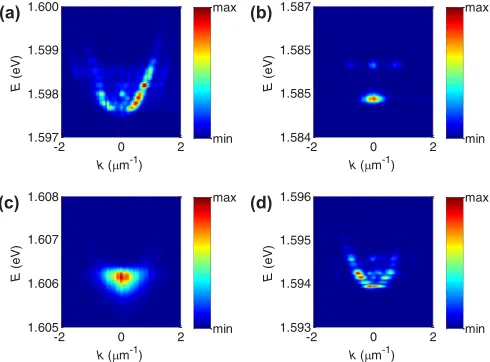
FIG. 3. Measured dispersion. (a) The same experimental condi-tions as in Figs.2(a)–2(c)(exciton-polariton condensation with top-hat pump profile at≈7K). Many quantized modes at different energy levels are clearly visible. (b) The same experimental conditions as in Figs.2(d)–2(f) (VCSEL lasing with top-hat pump profile at ≈200K). At least two quantized modes at different energies can be seen. (c) The same experimental conditions as in Figs.2(g)–2(i)

pseudovortices appear in both cases [Figs.2(a)and2(d)]. This indicates that [as the simulation in Fig. 1(d) also showed] they are not related to real vortices in a BKT condensate but rather they are artifacts from simultaneous emission at different energies Es so that it does not even matter if s

represents a BKT condensate or a VCSEL mode. If we slightly move the sample, the pseudovortices do not move with the sample but stay at a fixed position relative to the pump beam. This also shows that they cannot be real vortices trapped at defects of the sample. For comparison, we also performed similar measurements [4] with a Gaussian spatial pump profile, which has only a non-negligible overlap with the lowest mode1. In this case, condensation occurs only

into this mode [Fig.3(c)], and as expected, quasi-long-range order, which only decays very slowly has been observed, and no pseudovortices appeared [Figs.2(g)–2(i)].

VIII. SPECTROSCOPIC ENERGY-RESOLVED MEASUREMENT

Finally, to confirm that the simultaneous population of multiple modes reduces the spatial correlation, we performed an energy-resolved measurement which allows us to measure the correlation function of the individual modes (Fig.4). The setup is again similar to the previously used one [4,5], but this time the interference image is projected onto the entrance slit of a spectrometer [Fig.4(a)]. If this slit is widely opened and the grating aligned to act as a mirror (0th order), the spectrometer CCD camera records positionx- andy-resolved interference images [Fig.4(b)] in which we see interference fringes. However the spectrometer can also be used to perform positionx- and energyE-resolved measurements by closing the entrance slit so that only the signal with y≈0 enters the spectrometer and aligning the grating in such a way (first

-10 0 10

0 0.5 1

x( m)

g

(1

) (x

,-x

)

Fromx, yresolved Adding all modes Weighted average Phase sensitive average

x( m)

E

(m

eV)

-10 0 10

1596

1595

1594

x( m)

y

(m

)

-10 0 10

-10

0

10

(e)

(d) (c)

(f)

(a) (b)

9 10

8

2 1 4 3 6 7

5

Sample

Camera

Mirror Reflection prism

Pump laser

Leaking photons

Δ

L

Flipped signal

Signal Signal

Interference signal

-10 0 10

0 0.5 1

x( m)

g

(1

) (x

,-x

)

1 2 3 4 5 6 7 8 9 10

-10 0 10

0 200 400 600

x( m)

In

tens

it

y

(a.

u.

) I

(mode 6) measured

I(mode 6)

A

I(mode 6)

B max min

max

min

FIG. 4. Spectrometric-resolved interference measurement (exciton-polariton condensate with nearly constant density, created at≈8K with top-hat pumping). The estimated detuning was−8 meV, which is far red-detuned. (a) A spectroscopic interference setup. (b) A positionx -andy-resolved interference image (for one specific path-length differenceL). (c) A positionx- and energyE-resolved interference image, again for one specific path-length difference. Here, we can identify at least ten individual modes at different energy levels. (d) Evaluation for the sixth mode.I_measured(mode 6)has been measured at one specific path-length difference, whereasI_A(mode 6)andI_B(mode 6)have been calculated by using the measuredImeasured(mode 6)from many different path-length differences. (e) Visibilitiesg

(1) (modes)=I

(modes)

A /I

(modes)

B for the ten individual modes. (f)

order) that the one-dimensional interference signal which passes through the slit becomes spectrally resolved and is recorded as anx-andE-resolved image [Fig.4(c)]. The data in this image have been recorded with one specific path-length difference L, but the same kind of measurement has also been performed for many different path-length differences. In this spectrographic data, we can identify at least ten individual modes at different energy levels. The 11 horizontal lines show the (manually determined) borders between individual modes; this means, for example, we assume that any signal in the energy interval labeled 6 (which is between the sixth and the seventh horizontal lines) corresponds to the sixth quantized mode. Within each individual mode, interference fringes are again obvious, and if the measurement is repeated with changing path-length differences, these fringes move in the horizontalx direction. Figure4(d)depicts the evaluation for the sixth mode (but exactly the same evaluation has also been performed for all the other modes). The black line is determined as I_measured(mode6)(x)=E7

E6 Imeasured(x,E)dE where E6 andE₇ are the energy levels at which we drew the sixth and seventh lines in Fig.4(c) andImeasured(x,E) is the measured

spectrally resolved data in Fig.4(c). This means the black line shown in Fig. 4(d) corresponds to one specific path-length difference in the same way as the data shown in Fig. 4(c). The clear oscillations inI_measured(mode6)(x) correspond again to the interference fringes, and they appear to move in the horizontal x direction if one changes the path-length difference L. By performing the same integration for multiple path-length differences we getI_measured(mode6)(x,L), which is not shown in the figure, and by performing the sine fit explained in Eq. (10), we determine I_A(mode6)(x) and I_B(mode6)(x) as well as the (not shown) phaseϕ₀(mode6)(x). In Fig.4(e), we show the visibilities which we calculate for each of the ten individual modes as g(1)_(modes)(x,−x)=I_A(modes)(x)/I_B(modes)(x). The continuous black line in Fig. 4(f) displays the overall visibility which has been determined from the position-resolved measurement where only data within the area between the black lines in Fig. 4(b) have been considered. Since these data have been measured without spectral energy resolving, they are equivalent to the data shown in Fig. 2(c). The dotted line in Fig.4(f)has been calculated by undoing the energy resolution. For this, we performed the same evaluation as in Fig. 4(d), but we started by integrating over all energies from E1 to

E11. We notice that the dotted line which we get this way is

approximately the same as the continuous black line which we got without using any spectroscopy. This confirms that we can undo the spectroscopy by integrating over the energy of the

spectroscopic data. For comparison, the dashed line shows the average of the correlation of the individual modes, weighted by their intensities, this means

g_{weighted average}(1) (x,−x)=

10

s=1I (modes)

B (x)g

(1)

(modes)(x,−x)

10

s₌1I (modes)

B (x)

.

(12)

As expected, this weighted average which we get from eval-uating individual modes is more coherent than the correlation which has been determined without energy resolution. Finally, we use the correlations, intensities, and phases of the individual modes to calculate a phase-sensitive average (continuous gray line) using

g(1)_{phase-sensitive average}(x,−x)

=

10

s₌1I (modes)

B (x)g

(1)

(modes)(x,−x) exp iϕ (modes)

0

10

s=1I (modes)

B (x)

,(13)

which follows from Eq. (8); as expected it fits the non-energy-resolved data which confirm our theory.

IX. CONCLUSION

In conclusion, we showed through theoretical and experi-mental studies that an exciton-polariton BKT condensate with constant spatial density always consists of several modes. Their simultaneous presence causes a faster than expected decay of the spatial coherence (which can explain the result of Ref. [5] where the coherence decays with a power law whose exponent is larger than allowed under the BKT theory) and the appearance of pseudovortices which look similar to pinned vortices [16–19] or a vortex lattice [13] in a BKT phase. The higher spatial coherence of individual modes has been recovered through energy-resolved measurements, and we showed [Fig.4(f)and Eq. (9)] that the signals from different modes are incoherent from each other.

ACKNOWLEDGMENTS

This research has been supported by the Japan Society for the Promotion of Science (JSPS) through its “Funding Program for World-Leading Innovative R&D on Science and Technology (FIRST Program),” by Navy/SPAWAR Grant No. N66001-09-1-2024, and by National Science Foundation Grant No. ECCS-09 25549. W.H.N. acknowledges a Gerhard Casper Stanford Graduate Fellowship for support.

[1] H. Deng, G. S. Solomon, R. Hey, K. H. Ploog, and Y. Yamamoto,

Phys. Rev. Lett.99,126403(2007).

[2] Z. Hadzibabic, P. Kr¨uger, M. Cheneau, B. Battelier and J. Dalibard,Nature (London)441,1118(2006).

[3] J. Kasprzak, M. Richard, S. Kundermann, A. Baas, P. Jeambrun, J. M. Keeling, F. M. Marchetti, M. H. Szyma´nska, R. Andr´e, J. L. Staehli, V. Savona, P. B. Littlewood, B. Deveaud, and L. S. Dang,Nature (London)443,409(2006).

[4] W. H. Nitsche, N. Y. Kim, G. Roumpos, C. Schneider, M. Kamp, S. H¨ofling, A. Forchel, and Y. Yamamoto,Phys. Rev. B 90,

205430(2014).

[5] G. Roumpos, M. Lohse, W. H. Nitsche, J. Keeling, M. H. Szyma´nska, P. B. Littlewood, A. L¨offler, S. H¨ofling, L. Worschech, A. Forchel, and Y. Yamamoto,Proc. Natl. Acad. Sci. USA109,6467(2012).

[7] N. D. Mermin and H. Wagner, Phys. Rev. Lett. 17, 1133

(1966).

[8] V. L. Berezinski˘ı, Sov. Phys. JETP34, 610 (1972).

[9] J. M. Kosterlitz and D. J. Thouless,J. Phys. C: Solid State Phys.

6,1181(1973).

[10] Z. Hadzibabic and J. Dalibard,Riv. Nuovo Cimento Soc. Ital. Fis.34,389(2011).

[11] P. Nozi`eres, inBose-Einstein Condensation, edited byA. Griffin, D. W. Snoke, and S. Stringari (Cambridge University Press, Cambridge, UK, 1995).

[12] G. Roumpos, W. H. Nitsche, S. H¨ofling, A. Forchel, and Y. Yamamoto,Phys. Rev. Lett.104,126403(2010).

[13] F. Manni, T. C. H. Liew, K. G. Lagoudakis, C. Ouellet-Plamondon, R. Andr´e, V. Savona, and B. Deveaud,Phys. Rev. B88,201303(2013).

[14] C. Weisbuch, M. Nishioka, A. Ishikawa, and Y. Arakawa,Phys. Rev. Lett.69,3314(1992).

[15] H. Deng, G. Weihs, C. Santori, C. Bloch, and Y. Yamamoto,

Science298,199(2002).

[16] K. G. Lagoudakis, M. Wouters, M. Richard, A. Baas, I. Carusotto, R. Andr´e, L. S. Dang, and B. Deveaud-Pl´edran,

Nat. Phys.4,706(2008).

[17] K. G. Lagoudakis, T. Ostatnick´y, A. V. Kavokin, Y. G. Rubo, R. Andr´e, and B. Deveaud-Pl´edran,Science 326, 974

(2009).

[18] K. G. Lagoudakis, F. Manni, B. Pietka, M. Wouters, T. C. H. Liew, V. Savona, A. V. Kavokin, R. Andr´e, and B. Deveaud-Pl´edran,Phys. Rev. Lett.106,115301(2011).