Active Tectonics and Geomorphology of the central South Island, New Zealand: Earthquake Hazards of Reverse Faults

(1)

i

Active Tectonics and Geomorphology of

the central South Island, New Zealand:

Earthquake Hazards of Reverse Faults

A thesis submitted in partial fulfilment of the requirements for the degree of Doctor of Philosophy in Geology at the University of Canterbury by

Timothy Stahl

(2)

ii

FRONTISPIECE

“We started from a lonely valley, down which runs a stream called Forest Creek. It

is an ugly, barren-looking place enough ▬ a deep valley between two high ranges....We

went up a little gorge, as narrow as a street in Genoa, with huge black and dripping

precipices overhanging it, so as almost to shut out the light of heaven. I never saw so

curious a place in my life.”

-Samuel Butler, on the basis for the landscape in his novel

Erewhon

(A First Year in the Canterbury Settlement)

“First there is a mountain, then there is no mountain, then there is.”

-Donovan, on tectonic geomorphology

(3)

iii

ABSTRACT

Oblique continental collision between the Pacific and Australian Plates in the central South Island of New Zealand (between c. 44 and 46oS) results in distributed reverse faulting. Only a few of these faults have been studied in detail, highlighting a major knowledge deficit in the earthquake behaviour, magnitude potential and contribution to seismic hazard for many faults in this part of the orogen. Three reverse faults are investigated in detail in this thesis: the Moonlight Fault Zone (MFZ), the Fox Peak Fault and the Forest Creek Fault. Geochronologic approaches, including Schmidt hammer exposure-age dating, radiocarbon dating, and optically stimulated luminescence dating, are combined with paleoseismic trenching, fault surface trace mapping, analysis of GPS and LiDAR survey data, and numerical modelling to characterise the rupture behaviour of these faults.

(4)

iv

A trench on the range-bounding Forest Creek Fault, located in the hanging wall of the Fox Peak Fault, has had two to three earthquakes in the last c. 6 ka, with MRE and penultimate event ages overlapping those on the Fox Peak Fault. A Monte Carlo simulation that incorporates a distance-based probability for fault-to-fault rupture, fault geometry from field data and 3D modelling, and uncertainty in average slip is used to calculate probability density functions of moment magnitudes for the Fox Peak-Forest Creek fault system. Increased Coulomb stresses on the Forest Creek Fault from slip on the Fox Peak Fault are within the range reported for historic earthquake stress drops and confirm the feasibility of coeval rupture of these two imbricate faults. The results suggest that earthquakes 50-100% stronger than those predicted by empirical scaling laws need to be considered for the Fox Peak-Forest Creek system.

The 2010 Darfield (Canterbury) MW 7.1 earthquake caused coseismic landsliding in the

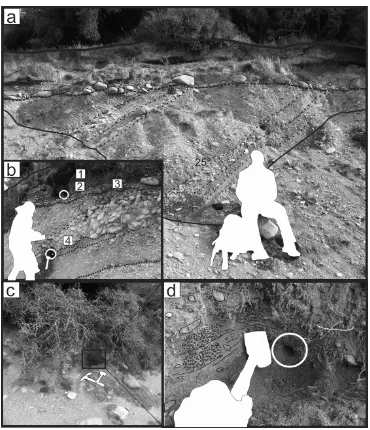
Harper Hills in the eastern foothills of the Southern Alps. Mapping, surveying, ground penetrating radar and trenching across the landslide head scarp indicate that failure was accommodated by combined bedding-controlled translation and toppling of decoupled basalt blocks. The lack of evidence for prior slip events over a time period that is likely to exceed the return period (1000– 2500 years) of peak ground accelerations at the site suggests that failure in the Harper Hills may be related to the fault-specific seismic source dynamics experienced in the Darfield earthquake.

(5)

v

TABLE OF FIGURES

Figure 1.1: Location map of SHD study sites around South Island, New Zealand ... 17

Figure 1.2: SHR-Age curves ... 26

Figure 1.3: SHR-Age data on a logarithmic scale ... 28

Figure 1.4: Matrix of Kruskal-Wallis test results for SHD data. ... 29

Figure 1.5: Climate and petrographic data for SHD study sites ... 31

Figure 1.6: Relationship of SHR to modal weathering rind thickness ... 35

Figure 2.1: Overview of study area in Otago ... 42

Figure 2.2: Field photo of shoreline terraces at Blanket Bay ... 44

Figure 2.3: LiDAR (dashed extent) and SPOT imagery of Kingston township at the southern end of Lake Wakatipu... 46

Figure 2.4: LiDAR and SPOT imagery of the Shotover delta area of Lake Wakatipu ... 47

Figure 2.5: SPOT imagery, RTK GPS data, OSL sampling locations, and terrace designations at the Greenstone River Fan ... 48

Figure 2.6: SPOT imagery, LiDAR and RTK GPS data collected at Bible Terrace and Blanket Bay ... 49

Figure 2.7: SPOT imagery Jack’s Point and Meicklejohns Bay ... 50

Figure 2.8: Range of SHD a-values for the study site ... 51

Figure 2.9: Algorithm to calculate SH exposure-age and error using Monte-Carlo rejection sampling ... 52

Figure 2.10: OSL sampling locations at the Greenstone River fan ... 53

Figure 2.11: Correlation of shorelines for all study sites and survey methods ... 55

Figure 2.12: Measured vs. modelled shoreline elevations ... 57

Figure 2.13: Elevation PDF and corresponding step function for Meiklejohns Bay ... 57

Figure 2.14: Cross-correlation plots for four study sites ... 58

Figure 2.15: Lake level reconstruction for Lake Wakatipu ... 61

(12)

xii

Figure 2.17: Finite element model of displacement on the Moonlight Fault ... 65

Figure 2.18: Cross-correlation technique applied to two surfaces containing correlated terraces with a uniform vertical offset ... 72

Figure 2.19: Cross-correlation technique applied to two flights of terraces with a progressively increasing vertical offset ... 73

Figure 3.1: Location and geology of the study site ... 79

Figure 3.2: Topography from 15 m DEM and locations of detailed field mapping ... 81

Figure 3.3: Tectonic and Quaternary geomorphic map of the Fox Peak Fault at Cloudy Peaks ... 83

Figure 3.4: A listric fault in Firewood Stream ... 84

Figure 3.5: Stream exposures of faults at Cloudy Peaks... 85

Figure 3.6: Tectonic and Quaternary geomorphic map of the Fox Peak Fault at the South Opuha River area ... 87

Figure 3.7: Outcrop of fan gravels underlying fluvial boulder lag at the South Opuha River ... 88

Figure 3.8: Outcrop of bedrock faults near the South Opuha River and fault plane solution for the area ... 88

Figure 3.9:Tectonic and Quaternary geomorphic map of the Fox Peak Fault at Ribbonwood Station ... 89

Figure 3.10: Tectonic and Quaternary geomorphic map of the Fox Peak Fault at Fox Peak and Lilydale Stations ... 91

Figure 3.11: Fault outcrops and dip variability on Fox Peak and Lilydale Stations ... 92

Figure 3.12: Overview of Butlers Creek faulting ... 93

Figure 3.13: Exposure of the EFPF at Butlers Creek ... 94

Figure 3.14: Outcrop of the EFPF just north of that shown in Fig. 3.13 ... 95

Figure 3.15: Investigation of possible FPF traces in Butlers Creek ... 97

Figure 3.16: The FCF at Forest Creek ... 99

Figure 3.17: Fault outcrop at Mt. Dobson ski field road... 100

Figure 3.18: Northward view of the southern FCF from Cloudy Peaks Station ... 101

Figure 3.19: Overview and extent of survey lines across the FPF ... 103

(13)

xiii

Figure 3.21: Fault scarp/terrace long profiles from the South Opuha River terraces. ... 105

Figure 3.22: Examples of fault scarp profiles from the Bray Segment ... 105

Figure 3.23: GPR of three Cloudy Peaks station fault scarps ... 106

Figure 3.24: Locations of OSL samples for determination of surface ages ... 108

Figure 3.25: Along-strike distribution of slip rates on the FPF and covariance with topography . 113 Figure 3.26:Trenches 1 and 2. See text and Appendix 4. ... 121

Figure 3.27: Trench 3 ... 123

Figure 3.28: Trench 4 ... 129

Figure 3.29: Determination of single event displacement from pooled net slips. ... 130

Figure 3.30: Trench 5 across the Forest Creek Fault ... 132

Figure 3.31: Event ages from paleoseismic trenching ... 137

Figure 3.32: Expected magnitudes of segmented and full-length ruptures of the Fox Peak and Forest Creek Faults ... 138

Figure 3.33: Best estimates of combined slip rates for the Fox Peak and Forest Creek Faults ... 139

Figure 3.34: Geomorphic map of Cloudy Peaks ... 142

Figure 3.35: Rapidly eroding silts and clays from Pliocene Kowai Formation gravels in Butlers Creek ... 143

Figure 3.36: Microtopographic (Total Station) survey of Trench 1 site ... 144

Figure 4.1: LANDSAT imagery and 15 m DEM block model of the field area ... 156

Figure 4.2: Determination of fault geometry for the listric rupture model ... 159

Figure 4.3: Algorithm for calculating MW in the planar fault model ... 161

Figure 4.4: Relocated hypocentres for the central South Island ... 163

Figure 4.5: Probability density functions of maximum MW for five rupture scenarios ... 164

Figure 4.6: Induced Coulomb stresses on the FCF from rupture on the FPF ... 165

Figure 5.1: Map and study site location ... 172

Figure 5.2: Local strong ground motion characteristics ... 173

Figure 5.3: Geologic and geomorphic map of the field area ... 174

(14)

xiv

Figure 5.5: Measurements of ground deformation in the Harper Hills landslide ... 177

Figure 5.6: Structural and kinematic measurements in the Harper Hills ... 178

Figure 5.7: Trench across the head scarp of the Harper Hills landslide ... 180

Figure 5.8: GPR Profiles ... 185

Figure 5.9:Cross-section and failure mechanism of the Harper Hills landslide... 189

Figure 5.10:Preservation potential of the head scarp ... 191

Figure 5.11:Influences on landslide failure and location ... 193

Figure 6.1: Map of the Lake Heron Fault at the Paddle Hill Creek fan ... 207

Figure 6.2: Google Earth image of the Terrace Spur Landslide ... 209

Figure 6.3: Field photo looking South along the scarp in the Terrace Spur wind gap ... 209

Figure 6.4: Field photograph of the main landslide body at Terrace Spur ... 210

(15)

xv

ACKNOWLEDGMENTS

During my Ph.D. study I was supported by a University of Canterbury Doctoral and International Doctoral Scholarships, for which I am grateful. My research was funded by the New Zealand Earthquake Commission, the Royal Institute of Chartered Surveyors (UK) and UC Mason Trust Grants.

First and foremost, I must thank my supervisory team for their guidance, friendship and timely reviews of my research. Mark Quigley provided valuable field training and feedback throughout, while allowing me to build this project from the ground up and always challenging me to do better. Mark, thanks for everything. It has been a pleasure to work with you and learn from you over the past four years.

Discussions in the field and office with Stefan Winkler provided valuable insights into Quaternary geomorphology and geochronology. Mark Bebbington tolerated my ambitious statistical schemes and helped mould them into useful tools in MatLab. Kari Bassett assisted with interpretation of trench logs. David Nobes assisted with GPR processing and interpretation.

I thank my office mates Brendan Duffy and Eric Bilderback for being excellent mentors, collaborators and friends. Ashton McGill, Sam McColl, Simon Cook and Tom Brookman all dedicated a week or more to field work on the Fox Peak, Forest Creek and Moonlight Faults. Their time and efforts were invaluable. Sharon Hornblow, Narges Khajavi, Travis Horton, David Nobes, Jarg Pettinga, Tristram Irvine-Finn, Matt Cockcroft, Josh Blackstock, Stefano the Italian, and Greg De Pascale all assisted with work in the field, which could not have been done without them.

This research benefitted from many useful discussions with colleagues at GNS and elsewhere, namely Phil Tonkin, David Barrell, Russ Van Dissen, Simon Cox, John Beavan, Simon Brocklehurst and Andy Nicol. The scientific extravaganza following the September 4th Darfield earthquake was memorable, due in part to being able to work with the quality crew of Nicola Litchfield, Pillar Villamor, Kevin Furlong, Chris Massey and others listed above.

(16)

xvi

The landowners of the Canterbury and Otago High Country have been wonderfully receptive and I thank them for allowing me access to their lands. In particular, the Aubreys of Ben McLeod Station, the Brays of Lilydale Station and the Murdochs of Cloudy Peaks Station were kind to allow several months of access over the past four years. The Cochranes of Hunter Valley Station and the Dennises of the Harper Hills kindly provided access on many occasions. It was a pleasure to deal with people as passionate about their land as I am.

I thank Ningsheng Wang at Victoria University of Wellington’s OSL Laboratory and Rafter Radiocarbon Laboratory at GNS for their efforts in dating my samples. Marco Olmos of the Queenstown Lakes District council kindly provided LiDAR of the Lake Wakatipu area. The editorial staffs and reviewers of three articles submitted for publication at GSA Bulletin, Earth Surface Processes and Landforms, and Geomorphology greatly improved the quality of the material presented in this thesis. Fault plane solutions were derived using Fault Kin5, Rick Allmendinger’s brainchild.

My friends David McConnel, Ashton McGill, Tom Brookman, Sam McColl, Mark Quigley, Narges Khajavi, Sharon Hornblow, Ben Mackey, Nick Riordan, Simon Cook, Brendan Duffy and Eric Bilderback helped keep me sane throughout, or, at least, I am indebted to their efforts.

(17)

1

THESIS PROLOGUE

Aims

On September 4th, 2010, at 4:30 a.m., an earthquake initiating on a blind reverse fault approximately 40 kilometres west of central Christchurch shook the city’s residents awake. The rupture jumped from the reverse Charing Cross Fault to strike-slip and oblique-normal fault segments before triggering another blind reverse fault rupture 20 seconds into the sequence (Holden et al. 2011; Beavan et al. 2012; Elliot et al. 2012; Bradley 2012). Widespread liquefaction in Christchurch, along with rock falls and ‘jumping’ boulders in the Port Hills, a landslide in the Harper Hills, and one of the best examples of strike-slip surface rupture ever recorded were all evident in the ensuing hours and days (Quigley et al. 2012; Bradley et al. 2012; Khajavi et al. 2012; Quigley et al. 2013; Stahl et al. 2014). Five months later, another oblique-reverse fault ruptured under the Port Hills, causing shaking that led to the deaths of 185 people and several tens of billions worth of damage to the city. The sources of the Darfield and Christchurch earthquakes were unknown to scientists before the events. It was first-hand experience of the importance of identifying and characterising active faults, including reverse faults in the New Zealand landscape.

The paucity of paleoseismic and geomorphologic data on reverse faults is not unique to New Zealand. Reverse faults are often blind, have discontinuous surface traces and contain zones of distributed, secondary faulting (c.f. Officers of the Geological Survey 1983; Rubin 1996; McCalpin 2009) that make surface studies difficult. There are relatively few historical, continental thrust and reverse faulting events with which to derive empirical scaling laws (e.g. Rubin 1996; Wesnousky 2008; Field et al. 2013). Geologically-derived slip rates often disagree with geodetic estimates due to fault trace obscurity in high relief landscapes and distributed deformation in the ranges adjacent to the fault (e.g. Wallace et al. 2007; Cox et al. 2012). Subsurface geometries can be complex, making fault traces and slip distributions at the surface appear relatively irregular compared to strike-slip ruptures. Additionally, seemingly unrelated faults at the surface may be linked at depth or be strongly influenced by regional stress fields, affecting the occurrence, and possibly concurrence, of earthquakes in a fault system (Lin and Stein 2004; Pollitz et al. 2003; Freed 2005).

(18)

2

to improve the scientific community’s understanding of reverse faults, I have also attempted to conduct primary source characterisation with the goal of providing robust data for inclusion in the New Zealand national seismic hazard model. Research questions and study sites were chosen accordingly.

Scientific Context

Relative motion between the Australian and Pacific plates in the central South Island of New Zealand is predominantly accommodated by slip on the Alpine Fault (Walcott 1998; Berryman et al. 2002). Geodesy and geology indicate that c. 75% of the 40-50 mm yr-1 oblique convergence is accommodated by slip on the Alpine Fault (Norris and Cooper 2001; Wallace et al. 2007; DeMets et al. 2010). With an average recurrence interval of 329 ± 68 years, and most recent event (MRE) of 1717 AD, the probability of an Alpine Fault rupture in the next 50 years is approximately 30% (Rhoades and Van Dissen 2003; Berryman et al. 2012). Expected magnitudes for a full-length rupture are MW 8.1 (De Pascale and Langridge 2012). More proximal known faults and distributed seismicity

contribute a higher component to the seismic hazard for the major population centres of the South Island (e.g. Stirling et al. 2008). In South Canterbury and Otago, this deformation and resulting contribution to seismic hazard are dominated by slip on NE-striking reverse faults.

Although there is clear geomorphic evidence of reverse faults preserved in the central South Island landscape, the geologic data collected thus far, with notable exceptions (Officers of the Geological Survey 1983; Van Dissen et al. 1994; Litchfield and Lian 2004; Amos et al. 2007; Amos et al. 2010; Amos et al. 2011) have been largely insufficient to validate presupposed slip rates, recurrence intervals and moment magnitudes. Geodesy has been invaluable in testing these assigned values but yields slip rates inconsistent with geologic studies where available (Wallace et al. 2007, Amos et al. 2010, this study). Moment magnitudes have mostly been assigned based on empirical scaling laws and not validated through paleoseismic trenching (e.g. Berryman et al. 2002). Recurrence intervals are also calculated based on scaling laws that have been primarily developed for oblique and strike-slip faults (Berryman et al. 2002; Stirling et al. 2013). Additionally, the probabilities of segmented fault ruptures are specified a priori and often informed by mapping alone. More work is required to test these critical parameters of the national seismic hazard model (NSHM).

(19)

3

proximity of the two faults and remarkable surface expression make this fault system an excellent place to test models of fault interaction and segment linkage. The fault system that ruptured in the Darfield earthquake (the Hororata Anticline, Greendale and Charing Cross Faults shown in Fig. P.1C) provided an excellent modern analogue of fault segment interaction. Coseismic ground cracks in the Harper Hills provided information on the return period of regional strong ground motions and the paleoseismicity of the Darfield earthquake sources. I have asked the following research questions regarding these faults (Table P.1):

[image:19.595.75.475.212.483.2]

(20)

4

Goal/Scientific Contribution Research Questions Relevant Chapter(s)

Obtain slip rates to identify segments and recent fault activity on the Fox Peak

Fault

How can the required age control be obtained for sequences of offset geomorphic markers?

Chapter 1

How are discontinuous geomorphic markers correlated and their offset measured across a fault?

Chapter 2

Is the paleoseismicity of a group of fault segments related to long-term range growth, and what are the implications for future

seismic hazard?

Chapter 3

Are geologically-derived slip rates consistent with current geodetic models of fault slip rates in the central South Island?

Chapters 2 & 3

Obtain ages and single-event displacements of earthquakes on fault segments to identify the

recurrence interval and magnitude potential of reverse fault systems

How can estimates of seismic hazard be improved by integrating field data into fault segmentation and fault-to-fault rupture

scenarios?

Chapter 3

How reliable are secondary (fault-induced) and indirect (off-fault, shaking-induced) records for determining the paleoseismicity of

the Fox Peak Fault and Darfield earthquake source?

Chapters 3 & 5

Investigate earthquake interaction and secular modulation of slip rates on

reverse faults

Is the Moonlight Fault active? What is the nature of strain heterogeneity and fault episodicity in Otago, and is it influenced

by glaciations?

Chapters 2 & 5

Does activity on the Fox Peak Fault influence the timing of earthquakes on the Forest Creek Fault?

Chapter 3 & 4

Thesis Format

Chapter 1 investigates the utility of applying Schmidt hammer exposure-age dating (SHD) to

fluvial terraces and outwash plains of New Zealand’s South Island. Studying reverse faults in the eastern Southern Alps of New Zealand presents the challenge of having few options for constraining absolute ages of features traversed by a fault. Detrital charcoal for radiocarbon is sparse and often washed out of fluvial systems during deposition, and luminescence requires well-exposed outcrops of (typically) fine material for dating. Cosmogenic dating is widely used, but requires either an impractical amount of samples from all offset features, or age-correlated features at all study sites. In a dynamic range-front environment, short-term variations in stream power make climatic or tectonic age-correlation of alluvial fans, landslides and river terraces unrealistic.

SHD is widely used in geomorphology, and when carefully calibrated, can provide meaningful ages for a range of landforms. It has never been used on river terraces prior to this thesis. The Schmidt hammer is ideal for obtaining ages from New Zealand river terraces for several reasons:

(21)

5

(ii) Large, rounded cobble and boulders of greywacke sandstone are often preserved at the surfaces of abandoned river terraces. The location of these terraces in the high energy environments of the Southern Alps ensures enough ‘surface clasts’ of suitable size are available for Schmidt hammer testing.

(iii) The known order of terraces in a sequence provides input data that can be used to further constrain ages (as opposed to other landforms, where relative order may be more ambiguous).

(iv) The lack of datable material in many eastern New Zealand river terraces has led to widespread usage of weathering-rind dating (e.g. Chinn 1981; Whitehouse et al. 1986; Knuepfer 1984, 1988; McSaveney 1992; Nicol and Campbell 2001). While proven effective, weathering-rind dating is destructive, time-intensive, requires surface clasts that can be removed to analyse rind thickness variability, and requires some subjectivity in what constitutes a rind. Additionally, rinds are often inexplicably absent from many boulders on a surface. SHD is non-destructive, conducted on in-situ surface clasts, and requires subjectivity only in that clasts must not move, break, or have evident shallow discontinuities during sampling.

I have calibrated the Schmidt hammer on terrace surfaces of known age and produced a new chronofunction for use in Torlesse greywacke. Chapter 1 explores the use of the technique in different sub-groups of Torlesse greywacke and weathering regimes in the South Island. Statistical protocols are developed for processing SH data and converting to SH values to absolute (numerical) ages.

Chapter 2 incorporates SHD (as well as absolute dating techniques), field mapping, surveying,

and LiDAR analysis to study the post-Last Glacial Maximum (LGM) activity of the Moonlight Fault in central Otago. The fault is situated in a zone c. 50-100 km from the plate boundary and stranded lake shorelines of Lake Wakatipu present ideal strain markers for studying the tectonic evolution of the basin. Studying their deformation is important for several reasons:

(i) The Moonlight Fault Zone (MFZ) cuts across the centre of Lake Wakatipu and its late Quaternary activity is uncertain. The MFZ has proposed late Quaternary traces and offsets (Wellman 1979; Turnbull 2000) but is mapped as inactive in GNS’s active fault database. Wallace et al. (2007) allow for 1 mm yr-1 convergence across the Moonlight Fault Zone in their geodetic model. The NSHM assigns a recurrence interval of c. 6 ka and expected magnitude of MW 7.6 for two separate

MFZ segments. Thus, there are conflicting views on its activity. It is essential for the future development of Queenstown and the Otago region to consider the hazard posed by the MFZ.

(22)

6

implies that strain is heterogeneously distributed in space and/or time throughout Otago. The high relief and depth of schist exhumation surrounding Wakatipu suggests that the area has had higher rock uplift rates than ranges to the East in the past. The shorelines of Lake Wakatipu, New Zealand longest lake in an orientation sub-perpendicular to the plate boundary, should reliably record the pattern of recent uplift for comparison.

(iii) Glacial loading and unloading have been shown to be mechanisms for the modulation of fault slip rates (Mörner 1978; Thorson 1996; Tsuboi et al. 2000; Stewart et al. 2000; Sauber and Molnia 2004; Hetzel and Hampel 2005; Hampel et al. 2009; Hampel et al. 2010). Given that Wakatipu contained a c. 1 km thick valley glacier as part of the Southern Alps ice-cap in the LGM (Barrell 2011), and is crossed by the MFZ, one could expect a glacially-modulated earthquake history to be recorded in the landscape.

I surveyed the lake shorelines using a combination of differential GPS (dGPS), real-time kinematic GPS (RTK), and existing Light Detection and Ranging (LiDAR) datasets. Dating was accomplished by calibrating SHD with optically stimulated luminescence (OSL) ages and an existing radiocarbon date of river terraces that correlate with the lake shorelines. I developed a numerical technique to correlate discontinuous shorelines observed in the LiDAR and dGPS from site to site to confirm my field observations of deformation. The results show that the shorelines have not been offset or tilted in the last c. 13-17 ka, revealing broad implications for the regional tectonics.

Chapter 3 investigates the paleoseismicity of the Fox Peak and Forest Creek fault systems in

South Canterbury. These two intersecting faults have long been recognised as having evidence of recent activity but have not been investigated in detail. The faults provide the ideal opportunity to study reverse fault development, segmentation and interaction. I used field mapping, surveying, trenching, dating and Monte Carlo modelling in MatLab to derive baseline fault parameters (length, sense, slip rates, recurrence intervals, single event displacements and segmentation) for the Fox Peak Fault. Slip rates and topographic analysis revealed discrete fault segments, which were subsequently trenched to obtain the ages of recent earthquakes. The results show that the structural development of the Fox Peak and Forest Creek Faults through time has increased the potential for large (MW 7+)

earthquakes.

Chapter 4 presents a Monte Carlo simulation approach for calculating moment magnitude

(23)

7

[image:23.595.73.523.136.604.2]

which have demonstrated a capacity, and perhaps the tendency, to jump onto arrays of nearby faults (e.g. Officers of the Geological Survey 1983; Rubin 1996; Lin and Stein 2004; Xu et al. 2009; Parsons et al. 2012; Field et al. 2013).

(24)

8

Chapter 5 presents the findings of research on the coseismic Harper Hills landslide that

occurred during the Darfield earthquake. The aim was to document and monitor the landslide as well as provide insight into the paleoseismicity of the region and utility of secondary (i.e. non-seismogenic) features in paleoseismology. I used GPR, structural and geomorphic mapping and trenching to characterise the kinematics and history of the landslide. The activation of the landslide was most likely related to source kinematics and dynamics that cannot be predicted by peak ground accelerations (PGAs) alone, highlighting the uncertainties in predicting earthquake impacts based on PGA return times from the NSHM. The required ground motion parameters for failure may be tied to the paleoseismicity of the Greendale and Hororata Anticline faults.

Chapter 6 summarises the main conclusions of this thesis. Preliminary data on high priority

active reverse faults are presented for further development of the central South Island reverse fault paleoseismic catalogue.

Appendices are included for individual chapters where appropriate and a Digital Supplementary Information file has been included for large spreadsheets (e.g. SHD data, survey shapefiles and regression statistics, slip and slip rates).

Logistical explanation for thesis structure

This is perhaps an unusual thesis in that a range of geologic phenomena are addressed and the field areas are separated by hundreds of kilometres. The topics move from Quaternary geochronology and numerical modelling, to short-term fault segmentation and paleoseismology, to long-term tectonic geomorphology and structure. How did such a thesis come to be?

I initially accepted an offer to complete a PhD on the paleoseismicity of the Fox Peak and Forest Creek Faults in early 2010. After initial reconnaissance and mapping, it was apparent that any research on fault segmentation would require a large number surface ages (and slip rates) outside the scope of site-to-site map correlations and outside the budget of the PhD. I enlisted my supervisor Stefan Winkler to assist with developing a calibrated-dating tool that could handle embedded surface clasts on river terraces. Over the course of several field trips and my own supervision of a University of Canterbury Summer Scholarship, I was able to produce new chronofunctions for Schmidt hammer exposure-age dating, and started putting them to use on the Fox Peak Fault in 2011.

(25)

9

Cook to look at the glacial history of the Lake Wakatipu basin. The work on the Moonlight Fault stemmed from 3 weeks in the field with Sam and Simon, followed by a fortuitous acquisition of LiDAR on shorelines I had already surveyed in the field.

The September 2010 Darfield earthquake had many impacts on the Canterbury landscape that required immediate documentation to ensure the quality of scientific data was not lost. My own involvement focused on the initial mapping of the surface trace and investigations into landslides in the Harper Hills and Banks Peninsula. Upon finding a null result in trenching of the landslide head scarp, I realised that this had broader implications for the paleoseismology of reverse faults, and decided to include the work in this thesis.

Scientific contributions arising from this PhD and related work

At the time of submitting this thesis, Chapters 1 and 5 have been published in peer-reviewed journals (Stahl et al. 2013; Stahl et al. 2014). Chapter 2 has been submitted and publication is pending a second stage of peer review. Some appendices in articles for publication have been moved into the main text of this thesis. The contents of all chapters have been widely presented at conferences, seminars and undergraduate lectures/laboratory sessions. I have co-authored and contributed to numerous other papers during my Ph.D. study involving the Darfield earthquake and surface rupture of the Greendale Fault (Quigley et al. 2010; Van Dissen et al. 2011; Barrel et al. 2011b; Quigley et al. 2012; Villamor et al. 2012; Duffy et al. 2013; Cook et al. 2013).

Originality

(26)

10

Deputy Vice-Chancellor’s Office

Postgraduate Office

Co-Authorship Form

This form is to accompany the submission of any thesis that contains research reported in co-authored work that has been published, accepted for publication, or submitted for publication. A copy of this form should be included for each co-authored work that is included in the thesis. Completed forms should be included at the front (after the thesis abstract) of each copy of the thesis submitted for examination and library deposit.

Please indicate the chapter/section/pages of this thesis that are extracted from

co-authored work and provide details of the publication or submission from the extract comes:

Chapter 1: Schmidt hammer exposure-age dating (SHD) of late Quaternary fluvial

terraces in New Zealand; Publication of same name in Earth Surface Processes and

Landforms, 2013.

Please detail the nature and extent (%) of contribution by the candidate:

Research was performed under the guidance of Stefan Winkler and Mark Bebbington.

Writing and scope benefitted from revisions with Mark Quigley and Brendan Duffy. All ideas,

execution of research, text and figures are those of the candidate, with input from coauthors.

Estimated candidate contribution 90%.

Certification by Co-authors:

If there is more than one co-author then a single co-author can sign on behalf of all The undersigned certifys that:

 The above statement correctly reflects the nature and extent of the PhD candidate’s contribution to this co-authored work

 In cases where the candidate was the lead author of the co-authored work he or she wrote the text

(27)

11

Deputy Vice-Chancellor’s Office

Postgraduate Office

Co-Authorship Form

Chapter 2: Post-glacial tectonic history of the Lake Wakatipu Basin and Moonlight

Fault; Submitted to Lithosphere, April 2014.

Estimated contributions in components of research:

Field work (planning, project aims, scope, execution): 50%

Analysis (survey processing, dating, modelling, other): 90%

Writing, literature review, formatting, revising: 90%

(28)

12

Deputy Vice-Chancellor’s Office

Postgraduate Office

Co-Authorship Form

Chapter 5-Coseismic landsliding during the 2010 Mw 7.1 Darfield (Canterbury)

Earthquake: Implications for paleoseismic studies of landslides; Accepted for publication

under same name in Geomorphology, 2014

Field work (planning, execution): 70%

Analysis of data: 80-90%

Writing: 90%

Eric Bilderback initiated landslide monitoring and mapping, and assisted with analysis.

Mark Quigley helped with mapping and trenching. David Nobes performed GPR and helped

with interpretation/writing of that section.

(29)

13

CHAPTER 1. SCHMIDT HAMMER

EXPOSURE-AGE DATING OF LATE QUATERNARY

(30)

14

1.1 Abstract

Schmidt hammer rebound values (R-values) are reported for surface clasts from numerically dated Holocene and Pleistocene fluvial terraces in the South Island of New Zealand. R-values are combined with previously obtained weathering rind, radiocarbon, terrestrial cosmogenic nuclide and luminescence terrace ages to derive SH R-value chronofunctions for greywacke clasts from four distinct locations. The results show that different weathering rates affect the form of the SH R-value vs. Age curve; however, a fundamental dependency between the two remains constant over timescales ranging from 102 to 105 years. Power law scaling constants suggest changes in clast weathering rates are primarily affected by climatic (precipitation and temperature) and sedimentologic variables (source terrane petrology). Age uncertainties of c. 22% of the surface age suggest that Schmidt hammer exposure-age dating (SHD) is a reliable calibrated-age dating technique for fluvial terraces.

1.2 Introduction

Geomorphic studies frequently utilise age dating of fluvial terraces and glacial outwash plains (e.g. Bull and Knuepfer 1987; Molnar et al. 1994; Amos et al. 2007, 2010; Barrell et al. 2011). Isotopic and radiogenic techniques have the ability to provide numerical ages but are typically expensive and labour intensive. River deposits that lack suitable organic material for radiocarbon dating, have complex mixing, burial and/or exposure histories that complicate terrestrial cosmogenic nuclide dating (TCND) or contain detritus that was not completely ‘bleached’ prior to deposition for luminescence dating may be challenging to date using these techniques.

Clasts exposed at or near the surface weather by chemical, physical and biological processes that collectively reduce the mechanical strength of the rock (e.g. Birkeland and Noller 2000; Walker 2005). Time-dependent variables like rock weathering rind thickness (e.g. Chinn 1981; Knuepfer 1988; McSaveney 1992; Oguchi and Matsukura 1999; Laustela et al. 2003), surface roughness (e.g. Benedict 1985), P-wave velocity (Crook and Gillespie 1986) and clast density (Maizels 1989) may be used to derive relative-ages for populations of surface clasts. The weathering-induced reduction of rock strength can also be measured using the Schmidt hammer (hereafter SH).

(31)

15

Matthews and Shakesby 1984; McCarroll 1989, 1991b,c; Winkler 2005; Shakesby et al. 2006, 2011; Matthews and Winkler 2012).

A geomorphic feature with independent, numerical age control can be used to quantify the relationship between SH R-values and exposure age. R-values of a population of surface clasts reflect the time-dependent mechanical degradation of the rock, and thus an approximate time since a presently stable surface was abandoned following erosion or aggradation. If numerical ages exist for a sequence of two or more features, then a chronofunction that relates SH R-values to surface exposure ages may be derived and used to estimate the surface ages for other undated deposits within the sequence (Shakesby et al. 2006; Winkler 2009; Matthews and Owen 2010). Geomorphic studies coupled with SH analyses have been used to produce calibrated-age curves for glacial, periglacial, mass movement, and alluvial fan deposits (e.g. McCarroll 1991a; Nesje et al. 1994a, b; White et al. 1998; Aa et al. 2007; Kellerer-Pirklbauer et al. 2008; Rode and Kellerer-Pirklbauer 2011; Shakesby et al. 2011), and polished bedrock surfaces (e.g. Gupta et al. 2009; Matthews and Owen 2010).

Previous studies have yielded strong correlations between average SH R-values and surface exposure ages within the Holocene (McCarroll 1987; Nicholas and Butler 1996; Winkler 2005; Matthews and Owen 2010; Shakesby et al. 2011). Only a few studies have applied SH exposure-age dating (SHD) to pre-Holocene surfaces, with variable results (e.g. White et al. 1998; Engel 2007; Sánchez et al. 2009). Shakesby et al. (2006) and White et al. (1998) are the only studies to apply SHD to fluvial deposits.

Fresh, fluvially-polished rock tends to yield the highest R-values for any given lithology (Ericson 2004; Gupta et al. 2009) and rounded clasts have the highest R-values of all sediment morphologies (McCarroll 1989; Shakesby et al. 2006), possibly as a result of minimal surface roughness (Williams and Robinson 1983; McCarroll 1989). Given the relatively high initial strength and low initial surface roughness of the lithologies and clasts present in New Zealand’s fluvial terraces (Read et al. 1999), SHD may be useful over a longer (pre-Holocene) timescale than commonly attempted.

(32)

16

1.3 Study Sites

The four study sites in the central South Island of New Zealand (Fig. 1.1A and B) were chosen because they contain well-dated Holocene and Pleistocene terraces, have similar clast lithologies and they span a range of contemporary climates. The ages used to calibrate SHD in this study are the best estimates of abandonment ages for the terraces. Terraces formed by lateral incision into pre-existing fan deposits, without subsequent aggradation or leaving a veneer of gravel prior to abandonment, may yield exposure ages older than the abandonment of the terrace tread (i.e. skewed to the age of deposition of the fan gravel). Weathering rind exposure-ages for terrace treads, as well as local terrace stratigraphy, suggest episodes of minor aggradation prior to abandonment for all of the terraces in this study (e.g. Bull 1990).

The Saxton River terraces (Fig. 1.1C) have been extensively studied in attempts to calculate slip rates on the cross-cutting Awatere Fault (Knuepfer 1988; McCalpin 1996; Mason et al. 2006). The site consists of six previously mapped terraces incised into a late Pleistocene (c. 16 ka) fan. For the purposes of our investigation, I differentiated between two terraces (T5a & T5b), previously mapped as T5, and separated by a c. 1 m riser. This was done to test the resolution of the SH in distinguishing between terraces formed in a short time period. All of the terraces except for T3 and T5a have been previously dated using weathering rinds, which produce consistently reliable results in New Zealand’s well-indurated Torlesse greywacke (Chinn 1981; Whitehouse et al. 1986; Knuepfer 1984, 1988; McSaveney 1992; Nicol and Campbell, 2001). Ages were inferred for terraces where maximum and minimum age control was available from adjacent terraces.

(33)

[image:33.595.74.502.68.641.2]

17

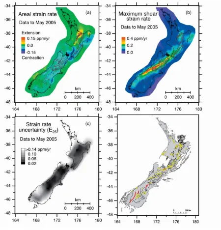
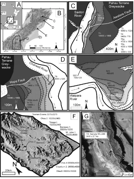
Figure 1.1: Location map of SHD study sites around South Island, New Zealand (A & B) and generalised geomorphic maps of study sites. All ages are given in years unless otherwise specified. (C) Saxton River terraces (modified after Mason et al. 2006); (D) Charwell River terraces (modified after Knuepfer 1984); (E)

Waipara River terraces (modified after Nicol and Campbell 2001); (F) 15m Digital Elevation Model (3x vertical exaggeration) of the Mackenzie basin and sites selected for sampling. (G) GeoEye aerial imagery of the Cloudy Peaks test site, showing location of OSL sample and paired fluvial terraces incised by stream flowing

(34)

[image:34.595.67.450.119.547.2]

18

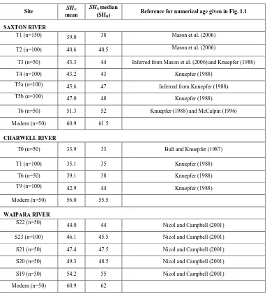
Table 1.1: Terrace names by study site, the amount of SH measurements (n) taken, SHN mean/median values and references for terrace ages given in Fig. 1.1. See text for discussion.

Site SHN

mean

SHN median (SHR)

Reference for numerical age given in Fig. 1.1

SAXTON RIVER

T1 (n=150) _39.0 38 Mason et al. (2006) T2 (n=100) 40.6 40.5 Mason et al. (2006)

T3 (n=50) 43.3 44 Inferred from Mason et al. (2006)and Knuepfer (1988) T4 (n=100) 43.2 43 Knuepfer (1988)

T5a (n=100) _45.6 ₄₇ _{Inferred from Knuepfer (1988)} T5b (n=100) _47.0 ₄₈ _{Knuepfer (1988)}

T6 (n=50) 51.3 52 Knuepfer (1988) and McCalpin (1996) Modern (n=50) 60.9 61.5

CHARWELL RIVER

T0 (n=50) 33.9 33 Bull and Knuepfer (1987) T1 (n=100) 35.1 35 Knuepfer (1988)

T6 (n=50) 39.1 38 Knuepfer (1988) T9 (n=100) _42.9 ₄₄ _{Knuepfer (1988)} Modern (n=50) 56.0 55.5

WAIPARA RIVER

S22 (n=50) _44.0 ₄₄ _{Nicol and Campbell (2001)} S23 (n=100) 46.1 45.5 Nicol and Campbell (2001) S21 (n=50) 47.4 47.5 Nicol and Campbell (2001) S20 (n=50) 49.3 48.5 Nicol and Campbell (2001) S19 (n=50) 54.2 55 Nicol and Campbell (2001) Modern (n=50) 60.9 62

(35)

19

stream also contains boulders of trachybasalt, either from the local Gridiron/Lookout Formations (Suggate 1958; Challis 1966) or from an unmapped volcanic member of the Torlesse greywacke. The weathering pattern of both lithologies is similar in surface clasts on abandoned terraces with the trachybasalt representing a relatively low proportion of the total clast count.

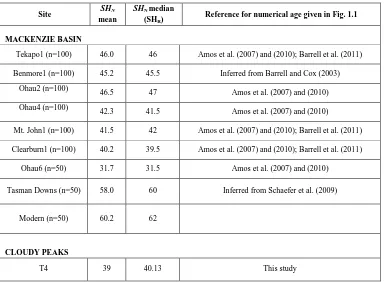
Table 1.1 (continued): Terrace names by study site, the amount of SH measurements (n) taken, SHN mean/median values and references for terrace ages given in Fig. 1.1. See text for discussion.

Site SHN

mean

SHN median (SHR)

Reference for numerical age given in Fig. 1.1

MACKENZIE BASIN

Tekapo1 (n=100) 46.0 46 Amos et al. (2007) and (2010); Barrell et al. (2011) Benmore1 (n=100) 45.2 45.5 Inferred from Barrell and Cox (2003)

Ohau2 (n=100) _46.5 ₄₇ _{Amos et al. (2007) and (2010)} Ohau4 (n=100) _42.3 _41.5 _{Amos et al. (2007) and (2010)}

Mt. John1 (n=100) 41.5 42 Amos et al. (2007) and (2010); Barrell et al. (2011) Clearburn1 (n=100) 40.2 39.5 Amos et al. (2007) and (2010); Barrell et al. (2011)

Ohau6 (n=50) 31.7 31.5 Amos et al. (2007) and (2010)

Tasman Downs (n=50) 58.0 60 Inferred from Schaefer et al. (2009)

Modern (n=50) 60.2 62

CLOUDY PEAKS

T4 39 40.13 This study

The Waipara River study site consists of between 5 cut-in-fill terraces that are all younger than 1 ka and are displaced by the Bobys Stream Fault (‘BSF’ in Fig. 1.1E) (Nicol and Campbell 2001; Campbell et al. 2003). The terraces consist primarily of a Torlesse greywacke gravel veneer (undifferentiated Pahau and Esk Head Melange sub-terranes) overlying a late Pleistocene outwash gravel strath surface. Nicol and Campbell (2001) used weathering rinds to date five of the terraces on site, as well as several others in the area with reliable results. Locally derived clasts of coarse-grained, Tertiary sandstone were identified on the three oldest terraces. On younger terraces and in the modern stream, coarse limestone boulders were readily identifiable. Some greywacke surface clasts on these terraces were coated with a calcium-carbonate film from the weathering limestone.

[image:35.595.67.452.207.489.2]

(36)

20

glaciofluvial outwash plains predominate. Glacial and periglacial features have been numerically dated using various techniques including OSL and TSL (thermally stimulated luminescence), TCND, and radiocarbon (Barrell and Cox 2003; Amos et al. 2007, 2010; Schaefer et al. 2009; Barrell 2011; Barrell et al. 2011). The ages of these features range from the ‘Little Ice Age’ to at least 100-150ka. Outwash plains are exceptionally preserved due to the dry climate and distance from the Main Divide, which allows reliable mapping of correlative deposits and features (e.g. Maizels 1989; Amos et al. 2007 and 2010; Barrell et al. 2011). Surface clasts are all Torlesse greywacke (Rakaia sub-terrane). Outwash plains in this study fall into five categories based on numerical ages: marine isotope stage (MIS) 5 or 6 (89 ± 16 ka); early MIS 2 (26.5 ± 4 ka); mid MIS 2 (inferred as 20.25 ± 10.25 ka); late MIS 2 (15.2 ± 2.3 ka); and Holocene (3.275 ± 3.275 ka) (Fig. 1.1F). Efforts were taken to sample where previously numerically dated samples had been taken; however, some samples were taken in locations of unknown age that have been mapped and correlated with dated units elsewhere (Amos et al. 2007, 2011; Barrell et al. 2011). Where minimum or maximum numerical ages were obtained, the age and error inferred for the surface was conservatively set midway between bounding units/surfaces of known age (Table 1.1). In addition to these four study sites, a test site at Cloudy Peaks, on the edge of the Mackenzie basin, was selected for comparison between OSL and SHD techniques. An OSL age of 24.8 ± 2.7 ka (Fig. 1.1G; Table 1.2) was obtained from fluvial silts overlying river gravel in a terrace located approximately 40m above stream level. Surface clasts used for SHD consist of Rakaia sub-terrane greywacke rocks.

Table 1.2: Optically stimulated luminescence results for T4 at the Cloudy Peaks test site- measured a-Value, Equivalent Dose, Cosmic Doserate, Total Doserate, and OSL Age.

Samplea Lat/Long a Value Deb Gyr

dDc/dtc Gyr/ka

dD/dtd OSL Age (ka)

Field Code

WLL946 -44.017,

170.693 0.05 ±0.01 88.74 ± 8.70

0.2162 ±

0.0108 3.57 ± 0.17

24.8 ± 2.7

T49611

a_{Sample preparation and measurements performed at the School of Earth Sciences, Victoria University of} Wellington, Wellington, New Zealand

b

Equivalent dose c

(37)

21

Table 1.2 (continued): OSL Sample description, water content and radionuclide content

Deposit Water

Content (%) K (%)

U (ppm) from 234_Th

U (ppm) from 226_Ra, 214_Pb,214_Bi

U (ppm) from 210_Pb

Th (ppm) from 208_Tl, 212_Pb,228_Ac

T4

sandlens 17.3

1.97 ±

0.04 2.69 ± 0.21 2.49 ± 0.12 2.08 ± 0.16

10.53 ± 0.12

1.4 Methodology

An N-type SH (hereafter SHN) with a calibrated impact energy of 2.207 N∙m (Proceq SA 2012)

was used in this study. Control of potential instrument error was constrained by pre- and post-sampling checks of correct calibration using a test anvil in order to detect instrumental deterioration during the measurement campaign. One SH impact was delivered on each clast for a minimum of 50 clasts per surface (e.g. Matthews and Shakesby 1984, Winkler 2005). This provides a statistically significant sample size and produces similar results to much larger sample sizes (Niedzielski et al. 2009). Although recently developed test designs with multiple sub-samples and an overall largely increased number of clasts measured at one site can significantly tighten the instrumental error margins (e.g. Shakesby et al. 2011, Matthews and Winkler 2012), the restricted availability of clasts suitable for testing and the character of my test sites preclude such attempts.

Where possible, two independent sets of 50 clasts were sampled on each surface to test for data consistency, as has been suggested for weathering rind studies (McSaveney 1992). A third test, during which the SHN operator was selective to sample only clasts with geomorphic stability indicators (i.e.

rock varnish, raised quartz veins, lichen cover), was conducted in instances where the surrounding geomorphology visibly suggested reworking or secondary deposition (e.g. T1 at the Saxton River site). This method weighted the dataset towards clasts with a more reliable exposure history without discarding data that may be relevant to the surface exposure age.

(38)

22

the surface), an additional attempt was made to resample the clast surface from another impact point. If the same problem was encountered, the clast was omitted from the dataset.

Clasts with less than 15 cm of rock exposed at the surface were avoided during sampling. Although ideally larger clasts/boulders are preferred with SH studies, the limited availability of clasts precluded an increase in this minimum size. While there is little constraint on subsurface clast geometry and edge effects in clasts of this size in the present study, I consider the chosen minimum of 15 cm exposed rock reasonable on the following bases:

i) Demirdag et al. (2009) showed in a series of tests that rocks from various lithologies with a minimum edge dimension greater than 11 cm yield consistent L-type SH R-values. The L-type SH has a lower impact energy than the SHN, and thus the minimum edge

dimension required for consistent results is likely somewhat higher for a SHN.

Nevertheless, the present cut off value of 15 cm is larger than suggested by Aydin (2009) for International Society of Rock Mechanics standards (100 mm at the point of impact for SHN), and is equivalent to those suggested in the ASTM (2005) (minimum 15 cm). ii) The terrace gravels I observed in outcrop rarely contained disk-shaped or ‘platy’ clasts,

which typically have much smaller edge dimensions than required for sampling.

iii) Every boulder was kicked before sampling to check for stability, and clasts that moved during sampling were considered unsuitable. Additionally, if a clast was chipped during sampling, or the SH sounded flat rather than resonant, indicative of a shallow discontinuity (as with disk-shaped clasts), the R-value was omitted from the dataset.

iv) Some of the impact energy during sampling may have been dissipated within the underlying soil as opposed to wholly within/on the clast being sampled. These effects are thought to be minimal, as most clasts sampled were firmly encased in soil. So long as the effect is constant (i.e. the average clast size and mechanical soil properties remain unchanged from site to site) the results should be internally consistent.

v) The SHN was chosen over devices with less impact energy (e.g. Equotip) due to

significantly smaller R-value variance (Viles et al. 2011) and a much more frequent usage in geomorphology in both New Zealand and elsewhere.

(39)

23

Catchment lithologies and proportional contributions to the fluvial system are assumed not to have changed over time.

For surface clasts with a simple exposure history, SH R-values are expected to be normally distributed (Winkler 2005, 2009) and the mean R-value from a series of measurements is the most often used proxy for the surface exposure age (e.g. Goudie 2006). In this study, slight differences were sometimes observed in the individual R-value distributions and dataset means when comparing individual tests on the same surface (n=50 per test) to each other and/or the combined dataset. Niedzielski et al. (2009) found that using the median increased R-value consistency and reduced the required sample size for a range of rock types. The median R-value (hereafter SHR) is less affected by

statistical outliers than the mean and is preferred in this study. Both mean and median values for the study sites are listed in Table 1.1.

A Kruskal-Wallis analysis of variance (ANOVA) test (Kruskal and Wallis 1952) was used to test for significant differences among SHR. The analysis was run as a multiple comparisons test

(comparing each median to every other median) at the 1σ level using a Dunn-Sidak correction (Sidak 1967). This is a much more conservative approach than identifying significant differences in a dataset sensu stricto but less conservative than multiple comparison tests with other adjustment techniques (e.g. Abdi 2007).

Age-SHR correlations are derived for the Saxton River terraces (Fig. 1.1C), Charwell River

terraces (Fig. 1.1D), Waipara River terraces (Fig. 1.1E), and Mackenzie basin outwash plains (Fig. 1.1F), with published age errors and 95% standard errors reported for age and SHR, respectively.

Climate data for the study sites were compiled along with petrologic information from Torlesse greywacke sub-terranes (Table 1.3). This was done to investigate possible changes in weathering rates due to differences in precipitation, temperature and source rock composition. Maximum temperature (°C) and precipitation data (mm) were downloaded from the National Institute of Water and Atmospheric Research (NIWA) CliFlo database as monthly averages over a thirty year time period. Climate stations that were nearest to the study sites (maximum 55 km) and in similar microclimates were chosen. For the Charwell River, Saxton River and Cloudy Peaks sites, temperatures were adjusted using an average New Zealand lapse rate of 0.5 °C/ 100 m (Norton 1985). Thirty year averages for each month were extrapolated to full year values (i.e. multiplied by 12) to obtain a range of possible annual precipitations (MAPmonth) and maximum mean temperatures (MATmonth). These are

(40)

24

weathering rates on temperature illustrates that climate extremes control long-term rates more so than lower average values (e.g. Velbel 1990).

Petrologic data for the Torlesse sub-terranes were compiled from a variety of sources and are reported as Quartz-Feldspar-Lithics (QFL) modal percentages (Table 1.3). For the Rakaia sub-terrane, averages were calculated from MacKinnon’s (1983) Petrofacies 1 through 4. The modal percentages of Petrofacies 5 (MacKinnon 1983; Roser and Korsch 1999) were used for the Pahau terrane, and supported by Barnes’ (1990) data. QFL percentages from greywacke within the Esk Head Melange are more difficult to quantify, but data from the greywacke blocks in the melange proper (Botsford 1983) and gradational contact into the Pahau terrane (Feary 1979) were taken as representative modal percentages.

Table 1.3: Thirty-year monthly averages of maximum temperature (°C) and precipitation (mm) extrapolated for a full year (MATmonth and MAPmonth, respectively). The data range is from 1981-2010, except for the Cloudy Peaks site/Fairlie weather station, where the only available data range was from 1951-1980. Petrologic data are given as modal percentages of Quartz-Feldspar-Lithics (QFL) for Torlesse greywacke sub-terranes.

Site Climate station Distance to study site (km) Elevation Difference (m)

MATJan MAPJan MATFeb MAPFeb MATMar MAPMar

Saxton Molesworth 9 70 21 521 20.9 548 18.5 586

Charwell Kaikoura

Aws 28 300 18.9 468 18.5 622 17.2 710

Waipara Waipara

West 3 0 23.8 691 23.7 491 21.6 544

Mackenzie Lake Tekapo, Air Safaris Variable; <55 Variable, not adjusted

21.6 624 21.3 396 18.8 564

Cloudy

Peaks Fairlie 14 200 20.6 708 20.4 564 18.6 888

Table 1.3 (continued)

Site MATApr MAPApr MATMay MAPMay MATJun MAPJun MATJul MAPJul MATAug MAPAug

Saxton 15.1 572 11.5 649 8.0 706 6.6 649 8.3 574

Charwell 14.7 666 12.7 679 10.5 900 9.4 1103 10.2 803

Waipara 19 672 15.6 434 12.8 635 12 646 13.4 755

Mackenzie 14.9 672 10.7 720 7 600 5.8 624 8.2 648

Cloudy

(41)

25 Table 1.3 (continued)

Site MAT Sep MAP Sep MAT Oct MAP Oct MAT Nov MAP Nov MAT Dec MAP Dec

Sub-terrane Q F L

Saxton 11.4 634 13.5 830 15.8 595 18.4 695 Pahau .26 .34 .40

Charwell 12.2 682 13.8 757 15.5 703 17.6 563 Pahau .26 .34 .40

Waipara 15.8 756 17.7 472 19.8 719 22.1 628 Pahau/Esk Head .40 .20 .40

Mackenzie 11.9 636 14.5 612 17.2 624 19.4 576 Rakaia .30 .50 .20

Cloudy Peaks 13.3 528 15.5 756 17.4 720 19.1 804 Rakaia .30 .50 .20

1.5 Results

1.5.1 SH Data

SHR values for all study sites decrease with an increase in terrace age (Fig. 1.2). In all three

curves, SHR can be correlated with age using a power law function of the simple form

(Eqn. 1.1)

where a and b are statistically estimated constants (Fig. 1.2A-C). The power law describes the SHR – age relationship over timescales ranging from 10

2

yr (Waipara) to 105 yr (Mackenzie basin) timescales. The curves are generally defined by a rapid decrease in SHR values from clasts within the

modern stream to clasts in the youngest terrace, followed by conformity to the power law (Eqn. 1.1). This implies that a short period (ca. 102 - 103 years for the study sites considered herein) of relatively rapid weathering occurs during and/or after the transfer of alluvium from an active channel into an ‘inactive’ terrace.

To test if the curves have a common slope, I used the statistical package (S)MATR and fit curves with a Major Axis (MA) regression (see Warton et al. 2006 for a full review). This was chosen in place of Ordinary Least Squares (OLS) fitting for the following reasons:

i) MA fitting uses a maximum likelihood estimation (MLE) of slope when deriving a common slope among different groups (e.g. different study sites). Using a MLE reduces Type 1 error (rejection of a potentially true hypothesis of common slope) and does not assume constant SHR variance with age (homoscedasticity) (Warton et al.

(42)

26

ii) MA fitting accounts for uncertainty in numerical age as well as SHR. An MA fitted

line optimises residuals perpendicular from the curve at the data point, as opposed to solely in the y (SHR) direction.

iii) MA is better suited to describing theoretical relationships between two variables; OLS is more appropriate when the goal is to predict y from x (Warton et al. 2006). The interest in this study is the former.

iv) In this study, MA yields values that generally agree with, but lie between the extremes of, OLS and standardised major axis fitting (Warton et al. 2006).

Figure 1.2: SHR-Age curves for (A) Saxton and Charwell River terraces; (B) Waipara River terraces; (C) Mackenzie basin outwash plains. Standard error of the median is approximated as 1.25 times the standard error