Applied Mathematics,2011, 2, 1159-1169
doi:10.4236/am.2011.29161 Published Online September 2011 (http://www.SciRP.org/journal/am)
Analysis of DAR(1)/D/s Queue with Quasi-Negative
Binomial-II as Marginal Distribution
Kanichukattu Korakutty Jose1, Bindu Abraham2
1Department of Statistics, St. Thomas College Palai Mahatma Gandhi University, Kottayam, India 2Department of Statistics, Baselios Poulose II Catholicose College,
Mahatma Gandhi University, Kottayam, India E-mail:[email protected], [email protected]
Received March 5, 2011; revised June 13, 2011; accepted June 20, 2011
Abstract
In this paper we consider the arrival process of a multiserver queue governed by a discrete autoregressive process of order 1 [DAR(1)] with Quasi-Negative Binomial Distribution-II as the marginal distribution. This discrete time multiserver queueing system with autoregressive arrivals is more suitable for modeling the Asynchronous Transfer Mode(ATM) multiplexer queue with Variable Bit Rate (VBR) coded teleconference traffic. DAR(1) is described by a few parameters and it is easy to match the probability distribution and the decay rate of the autocorrelation function with those of measured real traffic. For this queueing system we obtained the stationary distribution of the system size and the waiting time distribution of an arbitrary packet with the help of matrix analytic methods and the theory of Markov regenerative processes. Also we consider negative binomial distribution, generalized Poisson distribution, Borel-Tanner distribution defined by Frank and Melvin(1960) and zero truncated generalized Poisson distribution as the special cases of Quasi-Negative Binomial Distribution-II. Finally, we developed computer programmes for the simulation and empirical study of the effect of autocorrelation function of input traffic on the stationary distribution of the system size as well as waiting time of an arbitrary packet. The model is applied to a real data of number of customers waiting for checkout in an airport and it is established that the model well suits this data.
Keywords:Discrete Autoregressive Process of Order [DAR(1)], Multiserver ATM Multiplexer, Matrix
Analytic Methods, Markov Renewal Process, Markov Regenerative Theory, Teleconference Traffic, Quasi-Negative Binomial Distribution-II, Generalized Poisson Distribution, Borel-Tanner Distribution
1. Introduction
In B-ISDN/ATM network, IP packets or cells of voice, video, data are sent over a common transmission channel on statistical multiplexing basis. The performance analysis of statistical multiplexer whose input consists of a super- position of several packetized sources is not a straight- forward one. The difficulty in modeling this type of tra- ffic is due to the correlated structure of arrivals. A com- mon approach is to approximate this complex non re- newal input process by analytically tractable arrival pro- cess, namely discrete autoregressive process (DAR). The impact of autocorrelation in traffic processes on queueing performance measures such as mean queue length, mean waiting times and loss probabilities in finite buffers, can be very dramatic.
The DAR process, constructed and analyzed by Jacobs and Lewis [1] has developed into one of several standard tools for modelling input traffic in telecommunication networks. The discrete autoregressive process of order 1 [DAR(1)] is known to be a good model for VBR coded teleconference traffic as in Elwalid et al. [2]. Kamoun and Ali [3] modeled an ATM multiplexer as a discrete time multiserver queueing system with on-off sources and studied the transient and stationary distribution of the number of packets in the system.
multiserver queue fed by DAR(1) input. Kim et.al [7] derived mean queue size in a queue with discrete autoregressive arrival of order p.
In this paper we analyzed a discrete-time multi-server queue with s servers (s > 0) having deterministic service times (specifically, service time is 1) and the following arrival process: Let Am be the number of arrivals at time . Then Am = Am–1 with probability β; other-wise, Am is sampled independently from a quasi-negative binomial distribution-II. The stationary distribution of the waiting time in that queue is calculated numerically with a matrix analytic method. Specifically, the arrival process is first analyzed at embedded times when Am is sampled independently of Am–1 or when Am is less than the number of servers. This analysis reduces to an analy-sis of a Markov chain of M/G/1 type as presented in Neuts [8]. Then the stationary distribution of Am at gen-eral m is derived, which in turn gives the stationary dis-tribution of the waiting time.
0,1, 2,
m
The rest of the paper is arranged as follows. Quasi- Negative Binomial Distribution-II is described in Section 2. Queues with input traffic as DAR(1) with marginal Quasi-Negative Binomial-II is explained in Section 3. Analysis of DAR(1) /D/s queue with marginal Quasi- Negative Binomial Distribution-II is given in Section 4. The stationary distribution of the Markov renewal pro- cess is given in Section 5. Deriving the stationary distri- bution of system size and waiting time of an arbitrary pa- cket is explained in Sections 6 and 7. The quantitative effect of the stationary distribution of system size and waiting time on the autocorrelation function as well as the parameters of the input traffic is illustrated numeri- cally in Section 8. The application to real data set is given in Section 9.
2. Quasi Negative Binomial Distribution-II
The quasi-negative binomial distribution (QNBD) obtained by Janardan [9], Sen and Jain [10] has the probability mass function as
1 1 1 2 1 2
1 2
1 2 1 2
1 2 2
1 ! ; , , =
1 ! ! 1
for 0; > 0, > 0, > 0 and 0; < 0; = 0,1, 2
x
x n
n x p p xp P x n p p
n x p xp
p xp n p if p
p xp if p x
(1)
where x be the number of occurrences. When p2 = 0 the QNBD reduces to negative binomial distribution (NBD) and when n = 1, QNBD reduces to quasi geometric dist- ribution (QGSD) for n = 1. QNBD tends to the Consul and Jain’s [11] generalized Poisson distribution. But un- fortunately the moments of this distribution appear in an infinite series which is not suitable for summation. The
method of moments fails to provide quick estimates of its parameters. Hence Ahmad et al. [12] introduced a new model of quasi negative binomial distribution-II (QNBD- II). This new model has the probability mass function
1
2 1 1 1 2
1
2 1 2
2 1
1
1
1 1
for 0 < < 1 and 0 < < 1; = 0,1, 2
x
x n
np p p p xp
p x n x
np x p xp
np p x
(2)
When p20 this new model reduces to negative binomial distribution. The probabilities of QNBD-II de- creases with the successive occurrences. This tendency of probabilities suggests its possible applications in reliability, biometry, and survival analysis. The QNBD-II is uni-model and only its first moment (mean) appears in compact form. The lower and upper bound of Mode M is
1 11
1 1
1 1
< < , < 1
1 1
p n np
M p
p p
.
1
2 2= ,
1
np
Mean p
np
< 1
2.1. Remarks
1) Let X be a quasi-negative binomial variate with parameters (n, ) and pmf given by (2). If
such that 11 2 ,
p p
=
np
n
and np2= then the random variable X tends to generalized Poisson distribution with parameters
,
.2) Let X be a quasi-negative binomial variate with parameters (n, 1 2) and probability mass function is (pmf) is given by (2). If such that
,
p p
n n1= where then the random variable X tends to Borel-Tanner distribution defined by Frank and Melvin [13]
1=
2
p
3) Let X be a quasi-negative binomial variate with parameters (n, 1 2) and pmf given by (2), then zero- truncated quasi-negative-binomial distribution-II tends to zero-truncated generalized Poisson distribution as
.
,
p p
n
3. Queues with DAR(1) Arrivals with Quasi
Negative Binomial Distribution-II as
Marginal
The input ATM multiplexer with VBR coded telecon- ference traffic is assumed to be DAR(1) with quasi- negative binomial distribution-II as marginal. Let
Y t t: = 0,1, 2
be a sequence of i.i.d random vari- ables. Y(t) assumes positive values only and
= =
x
K. K. JOSE ET AL. 1161
Discrete Autoregressive Process of order 1 (DAR(1) is defined by the regression equa- tion as
: 0,1, 2,
X t t
0 == 1
0
1
, = 1, 2,X Y
X t Z t X t Z t Y t t
where are i.i.d Bernoulli random
variables with and
Z t t: 1, 2,3,
= 0P Z t
t = 1 = 1
= 0 < 1
P Z and Z t t
: 1, 2,3,
Y t t
isassumed to be independent of
. DAR(1) is determined by the parameter: 0,1, 2, and the distribution
b xx: = 0,1, 2,
of Y(t), so that
0 =
0X Y
=
1
with prob. with prob. 1X t X t
Y t
The properties of DAR(1) are as follows 1)
X t t
: 0,1, 2
is stationary2) The probability distribution of X(t) is the same as the distribution of Y(t)
= = x, = 0,1, 2 P X t x b x3) The autocorrelation function for X(t) at lag t is obtained as
=
0 ;
)= ,0
t
Cov X X t
t
Var X
t= 0,1, 2
the parameter is the decay rate of the autocorrelation function.
4. Analysis of DAR(1)/D/s Queue with
Quasi-Negative Binomial-II as Marginal
We assume that the input process is DAR(1) with quasi-negative binomial distribution-II distribution as the marginal distribution and there are s servers (s > 0) whose service occurs at constant rate. In this integer valued time queue, the time is divided into slots of equal size and one slot is needed to serve a packet by a server. We assume that packet arrivals occur at the beginning of slots and departures occur at the end of the slots. Here represents packet arrivals so that X(t) is the number of packets arriving at the beginning of the t slot.
X t t: 0,1, 2th
Let N(t) be the number of packets in the system say system size, immediately before arrivals at the beginning of the tth slot. Thenis a two dimensional Mar- kov process of M/G/1 queue type. The state space is
, : 0,1, 2
N t X t t
0 = , 0 , = 0,1, 2, 0,1, 2
nl n
n i n i E The number of phases is infinity. So the computation of stationary distribution of
is not easy to work out.
, : 0,1, 2
N t X t t
In practice by matrix analytical method and using the theory Markov regenerative processes, we compute the stationary distribution of the new process at the em- bedded epochs
t, = 0,1, 2
2< 3
t t as follows, we have 0 1
0 <t < <t
-1
0, = 0
= inf t > t :Z = 1 or 0 1 , = 1, 2
t
t X t s
Let
= , = 0,1, 2
N N t
0= J s
if = 0 = 1, 2,3 =
if = 1 = 1, 2,3
X t Z t
J
s Z t
The packet arrivals at and after t are independent of the information prior to t given J. From this, it is observed that
N J,
: =0,1, 2,
is the new Markov renewal process with state space
0,1, 2
0,1
E s
The probability transition matrix of the Markov renewal process is computed as follows.
1) For n0,1, 2and i0,1, , s1
max ,0 , with prob. ,
max ,0 , with prob. 1
n s i i n i
n s i s
2) For n0,1, 2
min , 1
0 0 =0
max , 0 , with prob. 0 1,
, with prob.
, (1 ) 1 1,
0, with prob. 1
, with prob. 0, > 0
i i
s n s
i n
i l
n s i i
b i s
n s i s
n s b s n i s
s b
n l s g l n l
g
where
0
1 if = 0 =
0 if 1 n
n n
0= s
g b
1 |= 1 , = 1, 2,
l i l i s
i l
g
b l1
1 2 1 2
1 2 2 2
1 2 1
0 1 1
0 2 1
3 2
0 0 0
0 0 0 0
s s s s s s s s
c s s s s s s s
B A A A
B A A A
B A A A
A A A A
A A A
A A
0 0 0
= , 0 i i s
A i s
s g
=0
= i ,1
i j
j
B
A i s<
We assume that the stability condition
=1=E X t = m mbm s
is satisfied.5. The Stationary Distribution of the
Markov Renewal Process
is obtained as above.
Where the elementary matrices are
0 i s
0 0 0
0 0 1 = 0 1 i i i A i b b s
Consider
N J,
, = 0,1, 2
, and
πni = limP N = ,n J =i n, 0, 0
= 0 N A i > n s 18
We apply
matrix analytic method as described below. The transition probability matrix P has infinite order, so that it would have to be truncated before we implement matrix analytic method. We assume that there exists some index N such that for all . That is we assume that the Markov chain does not jump more than N steps at a time so that the matrix is of finite order, see Latouche and Ramaswamy [14]. For a numerical illustration , consider the case when s = 5 and N = 14. Then the transition probability matrix P can be obtained as
N
0 i s 1
0 s
5 6 7 8 9 10 11 12 13 14 15 16 17 18 19
4 6 7 8 9 10 11 12 13 14 15 16 17
3 4 5 6 7 8 9 10 11 12 13 14 15 16 17
2 3 4 5 6 7 8 9 10 11 12 13 14 15 16
1 2 3 4 5 6 7 8 9 10 11 12 13 14 15
| |
5 | |
| |
| |
| |
B A A A A A A A A A A A A A A
B A A A A A A A A A A A A A A
B A A A A A A A A A A A A A A
B A A A A A A A A A A A A A A
B A A A A A A A A A A A A A A
0 1 2 3 4 5 6 7 8 9 10 11 12 13 14
0 1 2 3 4 5 6 7 8 9 10 11 12 13
0 1 2 3 4 5 6 7 8 9 10 11 12
0 1 2 3 4 5 6 7 8 9 10 11
0 1 2 3 4 5 6 7 8 9 10
| |
0 | |
0 0 | |
0 0 0 | |
0 0 0 0 | |
A A A A A A A A A A A A A A A
A A A A A A A A A A A A A A
A A A A A A A A A A A A A
A A A A A A A A A A A A
A A A A A A A A A A A
0 1 2 3 4 5 6 7 8 9
0 1 2 3 4 5 6 7 8
0 1 2 3 4 5 6 7
0 1 2 3 4 5 6
0 1 2 3 4 5
0 0 0 0 0 | |
0 0 0 0 0 | 0 |
0 0 0 0 0 | 0 0 |
0 0 0 0 0 | 0 0 0 |
0 0 0 0 0 | 0 0 0 0 |
0 0 0 0 0 | 0 0
A A A A A A A A A A
A A A A A A A A A
A A A A A A A A
A A A A A A A
A A A A A A
0 1 2 3 4
0 1 2 3
0 1 2
0 1
0
0 0 0 |
0 0 0 0 0 | 0 0 0 0 0 | 0
0 0 0 0 0 | 0 0 0 0 0 | 0 0
0 0 0 0 0 | 0 0 0 0 0 | 0 0 0
0 0 0 0 0 | 0 0 0 0 0 | 0 0 0 0
A A A A A
A A A A
A A A
K. K. JOSE ET AL. 1163
By arranging the transition probability matrix into (sxs) matrices we get
0 1 2
0 1 2
0 1
0
ˆ ˆ ˆ ˆ ˆ ˆ =
ˆ ˆ 0
ˆ 0 0
B B B
A A A
P A A A or equivalently
0 2 3
0 1 2
0 1
0
ˆ ˆ ˆ
ˆ ˆ ˆ =
ˆ ˆ 0
ˆ 0 0
B A A
A A A
P A A A
In general we can symbolize the transition matrix P as
0 1 2 1
0 1 2 1
0 1 2
0
ˆ ˆ ˆ ˆ ˆ ˆ ˆ ˆ = 0 ˆ ˆ ˆ
ˆ 0 0 0
n
n
n
B B B B
A A A A
P A A A
A
*= N s 1 1
n
s
or equivalently
0 2 3
0 1 2 1
0 1 2
0
ˆ ˆ ˆ ˆ
ˆ ˆ ˆ ˆ = 0 ˆ ˆ ˆ
ˆ 0 0 0
n
n
n
B A A A
A A A A
P A A A
A 1 2 3,
The elements of P can be written as
1 2 1 2 0 1 2 ˆ =
s s s s s s s
B A A
B A A
B
B A A
,
1 1 1
1 1 2
1 1 1 2
ˆ =
sn sn s n
sn sn s n
n
sn
s n s n
A A A
A A A
A
A A A
= 0,1, 2 ,
n n
1
ˆ
ˆ =n n , = 1, 2,
B A n n
A matrix P of the above structure is said to be of M/G/1 type, which underlines the similarity to the embedded Markov chain of the M/G/1 queue. With respect to the levels , the Markov chain is called skip free to the left, since in one transition the level can be reduced only by one.
By the matrix analytic method we proceed as follows. Step 1: Find the minimal nonnegative solution G of the matrix equation
=0
ˆ = n
n n
G
A GG can be given by the following iteration See Breuer [15] 0 1 0 1 1 =1 =1 = 0 ˆ = ˆ
= , = 2,
=
k n k n k
n k k
G
G A
G A G k
G G
G is a stochastic matrix ,and hence we can stop the iteration procedure when 1G.1 < reaches where
= 0.0001
. From this iteration we obtained the upper limit of k &let n=k1. From this we come to know the truncated index N at which G becomes stochastic
n
Step 2: Find
=0ˆ
= n n n n H
B Gand a positive row vector h satisfying hH =h Step 3:
0
1
0 1
=0 =1 =0
1 1 =0 = ˆ ˆ =
ˆ , = 1, 2
n n n
i i
n n i l n l i i l i
n i i i
x h
x x B G x A G
I A G n n
Step 4: Finally
π ,0, π , π 1 1,0 π 1 1,
= ,= 0,1, 2, ,
ns ns s n s n s s Cxn
n n
where C= nn=0xne1
and e is the s (s + 1) dimensionalcolumn vector whose components are all ones.
6. Stationary Distribution of
N t X t t
,
,
= 0,1, 2
renewal process and
N t t ,X t t : = 0,1,t 2
.
given
N ,X ,0< ,t N J , = n i,
isstochastically equivalent to
N t X t t
, : = 0,1, 2
given
N J0, 0=
n i,
Hence
N t X t t, : = 0,1, 2
is a discrete time Markov regenerative process with the Markov renewal sequence
N J, ,t : = 0,1, 2
.From the theorm See Kul-karni [16]
= lim , = , , = 0,1, 2
nj t
p P N t X t n j n j
of
N t X t, : = 0,1, 2t
are determined by
1 1 ts
, = , =0 =0 =
1 =0 =0
π 1 , = ,
π , = ,
li N t X t n j
l i t t
nj s
li l i
E N J l i
p
E t t N J l i
(3)We have
1 1= 1 , = , , =
1 if = ,0 1 and
if = ,0 1 and = if = , = and = 1
=
if = , > , and divides 0 otherwise.
t
t t N t X t n j
j
s
n l j s j
E N J
i j i s n l
b i s j s
b
i s j s n l
b i s j s n l
j s n l
, = l i n l The numerator of Equation (3) is
, =0
π π , 0
π
, =
1
π , 1
nj ns j ns s n j s
i j n i j s s i
b j
b
j s
b j s
1 s We have
1 1 =0 = , = ,1 if 0
1
if = 1
s
r r
r r s
E t t N J l i
i s
b b i s
1,The denominator of Equation (3) is
1 1
=0 =0 =0 =0 = 1
π π
1
s s
li ls r r
l i l r r s
b b
(4)where
=0π0 =0 is the stationary probabilityn l l l
vector of the Markov process
whose transition probability matrix is: = 0,1, 2 J
1
0 ,1
0 1 1
=0
= =
0 0 1
0 0 1
0 0 1
1
i j s
s
s r
r
P J j J i
b b b b
(5)The infinitesimal transition matrix of (5) is
Q =
1 0 1 =01 0 1
0 1 1
0 0 1
s r
r b b
b
The balance equations are
= 0 & e = 1
Q
By solving the balance equations we obtain the sta- tionary distribution of the Markov process
J: = 0,1, 2
as= =0
=
, 0 1
1 π = 1 , = 1 i r r s li l r r s b j s b i s b
(6)By substituting (6) into (4) we obtain the denominator of the right hand side of (3) as
1 r s=br
1
Theorem 6.1
The stationary distribution or the limiting pro- babilities
= lim , = , , , = 0,1, 2 nj t
p P N t X t n j n j
are given by
1 1 1 , =0π π , 0
π
, =
1
π , 1
nj ns j
ns s nj n j s i j n i j s s i
b j
b
j s p
b j s
s 1
where 1 =1 r =
K. K. JOSE ET AL. 1165
wise
j
7. Stationary Distribution of Waiting Time
of an Arbitrary Packet
Let W denote the waiting time of an arbitrary packet at steady state. Then for w= 0,1, 2.
P(W = w) = (Mean number of arrivals in a slot at steady state whose waiting time is w)/(Mean number of arrivals in a slot)
Suppose that there are n packets immediately before arrivals at the beginning of the tth slot and that the number of packet arrivals is j at the beginning of the tth slot, so that N(t) = n and X(t) = j. Then the number of packets whose waiting time is w among the ones who arrive at the beginning of the tth slot is
min 1 , , < < 1 min = , , =
0 other
s w n j sw n s w
n j sw s n sw n j
Therefore the mean number of arrivals in a slot at steady state whose waiting time w is
=0 = 1
1 1
= 1 =1
min = ,
min 1 ,
sw
nj n j sw n
s w
nj n sw j
p n j sw s
p s w n
Since the mean number of arrivals in a slot is , the following theorem is obtained from (7).
Theorem 7.1
The distribution of the waiting time W of an arbitrary packet is given by
=0 = 1 1 1
= 1 =1
1 min = ,
min 1 , ,
sw
nj n j sw n
s w
nj n sw j
P W w p n j sw s
p s w n j
8. Empirical Study
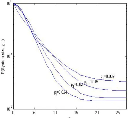
The complementary distribution function of the station- ary system size when when λ = 2.5 and β= 0.3, 0.5, 0.7 & 0.9 and the complementary distribution function of the stationary system size when β = 0.3 and p1 = 0.009, 0.0015, 0.02 &0.024 (p2 =0.0064, 0004, 0.002 & 0.0004) respectively are derived .
The parameter β gives the information on the strength of correlation of the input process. Stationary system size is larger for the large β (see Figure 1). Also stationary system size stochastically increases when the parameter
p1 of the input process decreases (see Figure 2).
The complementary distribution function of the wait- ing time of an arbitrary packet,when λ = 2.5 and β = 0.3,
[image:7.595.312.533.309.513.2]Figure 1. Complementary distribution function of the sta- tionary system size, when p1 = 0.0045, p2 = 0.0082, λ = 2.5.
Figure 2. Complementary distribution function of the sta- tionary system size, when λ = 2.5, β= 0.3.
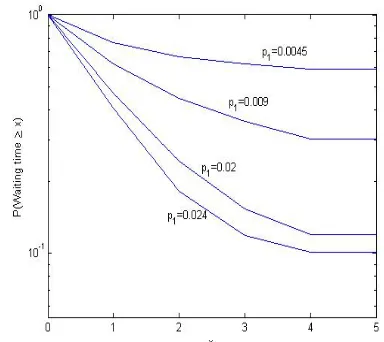
0.5, 0.7 & 0.9 and the complementary distribution func- tion of the waiting time when β = 0.3 and p1 = 0.009, 0.0015, 0.02 & 0.024 (p2 = 0.0064, 0004, 0.002 & 0.0004) respectively are derived.
Stationary waiting time of an arbitrary packet, is larger for large β (see Figure 3). Also stationary waiting time of an arbitrary packet, stochastically increases when the input parameter p1 decreases (see Figure 4). We assume the number of servers to be 3
Tables 1-3 display the stationary probabilities of the system size for different values of p p1, 2,& .
Tables 4 and 5 display the stationary probabilities of waiting time of an arbitrary packet for different values of
Figure 4. Complementary distribution function of the wait-ing time of an arbitrary packet, when β= 0.3.
[image:8.595.58.539.310.504.2]Figure 3. Complementary distribution function of the wait-ing time of an arbitrary packet,when p1 = 0.009, p2 = 0.0064.
Table 1. Showing the values of distribution of stationary system size P(n, j) for λ = 2.5, β= 0.1, p1 = 0.0045, p2 = 0.0082 and s = 3.
j
n 0 1 2 3 4 5 6 7 8
0 0.5148 0.1005 0.0460 0.0264 0.0158 0.0114 0.0086 0.0067 0.0054
1 0.0460 0.0090 0.0090 0.0026 0.0031 0.0011 0.0008 0.0006 0.0005
2 0.0135 0.0026 0.0495 0.0007 0.0007 0.0014 0.0002 0.0001 0.0001
3 0.0104 0.0021 0.0009 0.0005 0.0004 0.0003 0.0010 0.0001 0.0001
4 0.0081 0.0016 0.0007 0.0004 0.0003 0.0003 0.0002 0.0007 9.E - 04
5 0.0005 0.0012 0.0005 0.0003 0.0002 0.0001 0.0001 0.0001 0.0006
6 0.0043 0.0009 0.0004 0.0002 0.0001 0.0001 0.0001 8.E-04 0.0001
7 0.0034 0.0006 0.0003 0.0001 0.0001 0.0001 8.E - 04 6.E-04 5.E - 04 8 0.0028 0.0005 0.0002 0.0001 0.0001 8.E-04 6.E - 04 0.0001 4.E - 04
9 0.0028 0.0005 0.0002 0.0001 0.0001 8.E-04 7.E - 04 5.E - 04 4.E - 04
10 0.0023 0.0004 0.0002 0.0001 9.E - 04 6.E-04 5.E - 04 4.E - 04 8.E - 04 11 0.0019 0.0003 .00017 00011 7.E - 04 5.E-04 4.E - 04 3.E - 04 3.E - 04
[image:8.595.63.540.529.723.2]
Table 2. Showing the values of distribution of stationary system size P(n, j) for λ = 2.5, β = 0.3, p1 = 0.009, p2 = 0.0094 and s = 3.
j
n 0 1 2 3 4 5 6 7 8
0 0.5875 0.1148 0.1413 0.0300 0.0020 0.0014 0.0010 0.0008 0.0006 1 0.0009 0.0001 0.0100 0.0004 0.0018 2.E - 04 1.E - 04 1.E - 04 1.E - 04
2 0.0097 0.0046 0.0682 00206 0.0040 0.0054 0.0005 0.0003 0.0003
3 0.0001 3.E - 05 2.E - 05 4.E - 05 0.0014 2.E - 05 0.0009 1.E - 05 9.E - 05
4 8.E - 05 1.E - 05 1.E - 05 3.E - 05 0.0013 0.0011 1.E - 05 0.0007 7.E - 05
5 2.E - 05 1.E - 05 7.E - 05 2.E - 05 0.0012 2.E - 05 2.E - 05 1.E - 05 0.0006
6 3.E - 05 1.E - 05 8.E - 05 2.E - 05 0.0010 0.0010 0.0008 1.E - 05 9.E - 05
7 3.E - 05 6.E - 06 5.E - 06 1.E - 05 0.0009 1.E - 05 1.E - 05 1.E - 06 1.E - 06
8 3.E - 05 6.E - 06 5.E - 06 1.E - 05 0.0009 1.E - 05 1.E - 05 1.E - 06 1.E - 06
9 0.0016 0.0007 0.0005 0.0003 0.0002 0.0002 0.0002 0.0001 0.0007
10 2.E - 05 4.E - 06 3.E - 06 1.E - 05 0.0007 0.0008 1.E - 05 2.E - 06 0.0005
11 1.E - 05 3.E - 06 1.E - 06 9.E - 06 0.0006 1.E - 05 2.E - 06 1.E - 06 8.E - 06
K. K. JOSE ET AL. 1167
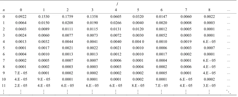
Table 3. Showing the values of distribution of stationary system size P(n, j) for λ = 2.5, β = 0.3, p1 = 0.024, p2 = 0.0004 and s = 3.
j
n 0 1 2 3 4 5 6 7 8
0 0.0922 0.1530 0.1759 0.1358 0.0605 0.0320 0.0147 0.0060 0.0022
1 0.0064 0.0150 0.0208 0.0190 0.0266 0.0040 0.0020 0.0008 0.0003
2 0.0603 0.0089 0.0111 0.0115 0.0131 0.0120 0.0012 0.0005 0.0001
3 0.0024 0.0060 0.0077 0.0073 0.0072 0.0030 0.0052 0.0003 0.0001
4 0.0013 0.0032 0.0044 0.0041 0.0040 0.004 0 0.0010 0.0019 6.E - 05
5 0.0001 0.0017 0.0021 0.0022 0.0021 0.0010 0.0006 0.0003 0.0007
6 0.0004 0.0010 0.0013 0.0013 0.0012 0.0010 0.0017 0.0002 0.0001
7 0.0002 0.0005 0.0007 0.0007 0.0006 0.0001 0.0004 0.0001 6.E - 05
8 0.0001 0.0002 0.0003 0.0003 0.0003 0.0004 0.0002 0.0006 4.E - 05
9 7.E - 05 0.0001 0.0002 0.0002 0.0002 0.0002 0.0005 0.0001 4.E - 05
10 4.E - 05 9.E - 05 0.0001 0.0001 0.0001 0.0002 0.0001 6.E - 05 0.0002
11 2.E - 05 4.E - 05 6.E - 05 6.E - 05 6.E - 05 8.E - 05 7.E - 05 4.E - 05 3.E - 05
Table 4. Showing the values of the distribution of waiting time of an arbitrary packet P(W = ω) for different values of βand λ
= 2.5, p1 = 0.009, p2 = 0.0064 and s = 3.
β
ω 0.1 0.3 0.5 0.7 0.9
0 0.2332 0.2326 0.2306 0.2270 0.2211
1 0.1096 0.0991 0.0832 0.0598 0.0245
2 0.0499 0.0473 0.0432 0.0359 0.0187
3 0.0280 0.0289 0.0285 0.0257 0.0158
[image:9.595.56.539.460.589.2]
Table 5. Showing the values of the distribution of waiting time of an arbitrary packet P(W = ω) for different values of p1,β =
0.3, and s = 3.
p2
0.0082 0.0064 0.004 0.002 0.0004
p1
ω 0.0045 0.009 0.015 0.02 0.024
0 0.2326 0.3748 0.4847 0.5303 0.5944 1 0.0991 0.1790 0.2407 0.2267 0.2229 2 0.0473 0.0898 0.1102 0.0890 0.0636 3 0.0289 0.0543 0.0569 0.0341 0.0179
9. Analysis and Modeling of a Data Set
In this section we apply the model to a data on the number of initially waiting customers for checking in an airport for a time period of 30 minutes each
. The data was collected from morning 8.00 A.M to 11.30 P.M for one week. This includes all the busy periods as well as idle periods. The data is taken from the file customer checkout.xlsx available in [17]. Table 6 gives the frequency distribution of the corre-
sponding data, where x is the number of customers initially waiting for the service.
t= 0,1, ,30In the present paper we assumed the number of arrivals as DAR(1) with marginal Quasi Negative Binomial II distribution. Thus the data set can be fitted to the the Quasi Negative Binomial II distribution as follows.
Table 6. Table showing the frequency distribution of the number of customers waiting for checkout.
x frequency x frequency
0 43 12 8 1 49 13 2 2 47 14 5 3 44 15 3
4 29 16 3 5 22 17 2 6 30 18 0 7 14 19 1
8 15 20 0 9 5 21 1 10 8 22 1
11 4 Total 336
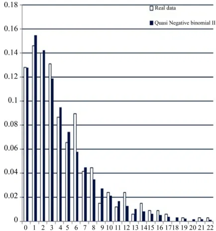
bution with parameter p1 = 0.021 and p2 = 0.00513 is a good fit for the given data. Here the calculated value of the K.S. test statistic is 0.017857 and the critical value corresponding to the significance level 0.01 is 0.088924, showing that the assumption for number of arrivals follow Quasi Negative Binomial II distribution is valid (see Figure 5).
By applying matrix analytic method we obtain the stationary distribution of system size and waiting time of an arbitrary customer for the Quasi Negative Binomial II/D/s queue. Here the mean = λ =4.3125. To satisfy the stability condition we assume the number of servers as . Also we assume the value of autocorrelation func- tion
= 5
s
= 0.1
, 1 and 2 . Tables 7 and 8 display the stationary distribution of waiting time of an arbitrary customer and system size.
= 0.021
[image:10.595.55.288.103.291.2]p p = 0.00513
Figure 5. The Probability histogram of real data and the Quasi Negative Binomial II distribution with p1 = 0.021 and
p2 = 0.00513.
Table 7. Table showing the stationary distribution of wait- ing time of an arbitrary customer P(W =ω)when β = 0.1, λ = 4.3125, s = 5.
w p(w)
0 0.2832
1 0.1195
2 0.0589
3 0.0380
[image:10.595.307.538.395.490.2]
Table 8. Table showing the stationary distribution of system size P(n, j) when β = 0.1,λ = 4.3125, s = 5.
j
n 0 1 2 3 4 5 6 7 8 9
0 0.102 0.123 0.114 0.094 0.075 0.058 0.041 0.031 0.024 0.019
1 0.007 0.009 0.008 0.008 0.008 0.004 0.003 0.002 0.001 0.001
2 0.005 0.006 0.007 0.006 0.007 0.003 0.002 0.001 0.001 0.001
3 0.004 0.005 0.005 0.005 0.005 0.003 0.002 0.001 0.001 0.001
4 0.004 0.005 0.005 0.005 0.005 0.003 0.002 0.001 0.001 0.001
5 0.003 0.003 0.003 0.003 0.003 0.002 0.001 0.031 0.000 0.000
6 0.002 0.003 0.003 0.003 0.003 0.001 0.001 0.000 0.000 0.000
7 0.002 0.002 0.002 0.002 0.002 0.0033 0.000 0.000 0.000 0.000
8 0.001 0.001 0.001 0.001 0.001 0.001 0.000 0.000 0.000 0.000
9 0.001 0.001 0.001 0.001 0.001 0.001 0.007 0.000 0.000 0.000
[image:10.595.56.545.521.720.2]K. K. JOSE ET AL. 1169
1
0. Conclusions
In this paper we analyze DAR(1)/D/s queue with Quasi- Negative Binomial Distribution-II as the marginal distri- bution. Based on the matrix analytic methods and by using the theory of Markov regenerative processes, we obtained the stationary distributions of the system size and the waiting time of an arbitrary packet. From the definition of autocorrelation function we can say that the larger the parameter β, the slower the decay of the autocorrelation of the input process. So it is expected that stationary system size and waiting time for the case of large βare stochastically larger than those for the case of small β. Also the stationary system size and waiting time increases when the input parameter p1 decreases.
11. References
[1] P. A. Jacobs and P. A.W. Lewis, “Discrete Time Series generated by Mixtures III: Autoregressive Processes (DAR(p)),” Naval Postgraduate School, Monterey, 1978. [2] A. Elwalid, D. Heyman, T. V. Laksman, D. Mitra and A.
Weiss, “Fundamental Bounds and Approximations for ATM Multiplexers with Applications to Video Telecon-ferencing,” IEEE Journal of Selected Areas in Commu-nications, Vol. 13, No. 6, 1995, pp. 1004-1016.
doi:10.1109/49.400656
[3] F. Kamoun and M. M. Ali, “A New Theortical Approach for the Transient and Steady—State Analysis of Multis-erver ATM Multiplexers with Correlated Arrivals,” 1995 IEEE International Conference on Communications, Vol. 2, 1995, pp. 1127-1131. doi:10.1109/ICC.1995.524276
[4] G. U. Hwang and K. Sohraby, “On the Exact Analysis of a Discrete Time Queueing System with Autoregressive Inputs,” Queueing Systems, Vol. 43, No. 1-2, 2003, pp. 29-41. doi:10.1023/A:1021848330183
[5] G. U. Hwang, B. D. Choi and J. K. Kim, “The Waiting Time Analysis of a Discrete Time Queue with Arrivals as an Autoregressive Process of Order 1,” Journal of
Ap-plied Probability, Vol. 39, No. 3, 2003, pp. 619-629. [6] B. D. Choi, B. Kim, G. U. Hwang and J. K. Kim, “The
Analysis of a Multiserver Queue Fed by a Discrete Auto-regressissive Process of Order 1,” Operations Research Letters, Vol. 32, No. 1, 2004, pp. 85-93.
doi:10.1016/S0167-6377(03)00068-3
[7] J. Kim, B. Kim and K. Sohraby, “Mean Queue Size in a Queue with Discrete Autoregressive Arrivals of Order p,” Annals of Operations Research, Vol. 162, No. 1, 2008, pp. 69-68. doi:10.1007/s10479-008-0318-1
[8] M. F. Neuts, “Structured Stochastic Matrices of the M/G/1 Type and Their Applications,” Dekker, New York. 1989.
[9] K. G. Janardhan, “Markov-Polya urn Model with Pre- Determined Strategies,” Gujarat Statistical Review, Vol. 2, No. 1, 1975, pp. 17-32.
[10] K. Sen and R. Jain “Generalized Markov-Polya urn Model Withpre-Determined Strategies,” Journal of Sta-tistical Planning and Inference, Vol. 54, 1996, pp. 119- 133. doi:10.1016/0378-3758(95)00161-1
[11] G. C. Jain and P. C. Consul, “A Generalized Negative Bi- nomial Distribution,”Society for Industrial Mathematics, Vol. 21, No. 4, 1971, pp. 501-513. doi:10.1137/0121056
[12] S. B. Ahmad, A. Hassan and M. J. Iqbal, “On a Quasi Negative Binomial Distribution–II and Its Applications,” Preprint,2010.
[13] A. H. Frank and A. B. Melvin, “The Borel-Tannerdistri- bution,” Biometrica,Vol. 47, No. 1-2, 1960, pp. 143-150. [14] G. Latouche and V. Ramaswamy, “Introduction to Matrix
Analytical Method in Stochastic Modelling,”Society for Industrial Mathematics, Pennsylvania, 1991.
[15] L. Breuer and D. Baum “An Introduction to Queueing Theory and Matrix Analytic Method,” Springer, Berlin, 2004.
[16] V. G. Kulkarni “Modelling and Analysis of Stochastic Systems,” Chapman & Hall, London, 1995.