A Parametric Approach to the Bi criteria Minimum Cost Dynamic Flow Problem

doi:10.4236/ojdm.2011.13015 Published Online October 2011 (http://www.SciRP.org/journal/ojdm)

A Parametric Approach to the Bi-criteria Minimum

Cost Dynamic Flow Problem

Mircea Parpalea

National College Andrei Şaguna, Braşov, Romania E-mail: [email protected]

Received June 26,2011; revised July 28, 2011; accepted August 10, 2011

Abstract

This paper presents an algorithm for solving Bi-criteria Minimum Cost Dynamic Flow (BiCMCDF) problem with continuous flow variables. The approach is to transform a bi-criteria problem into a parametric one by building a single parametric linear cost out of the two initial cost functions. The algorithm consecutively finds efficient extreme points in the decision space by solving a series of minimum parametric cost flow problems with different objective functions. On each of the iterations, the flow is augmented along a cheap-est path from the source node to the sink node in the time-space network avoiding the explicit time expan-sion of the network.

Keywords:Dynamic Network, Parametric Cost, Bi-Criteria Minimum Cost Flow, Successive Shortest Path

1. Introduction

Classical (static) network flow models have been well known as valuable tools for many applications [1] and therefore efficient algorithms have been developed. However, they fail to capture the dynamic property of many real-life problems, such as traffic planning, pro-duction and distribution systems, communication sys-tems, and evacuation planning. Dynamic flows are widely used to model different network-structured, deci-sion-making problems over time (see for example [2] and [3]), but because of their complexity, dynamic flow models have not been investigated as well as classical flow models. The time is an essential component, either because the flows take time to pass from one location to another, or because the structure of the network changes over time.

On the other hand, in many combinatorial optimiza-tion problems, the selecoptimiza-tion of the optimum soluoptimiza-tion takes into account more than one criterion. For example, in transportation problems or in network flows problems, the criteria that can be considered are the minimization of the cost for selected routes, the minimization of arrival time at the destinations, the minimization of the deterio-ration of goods, the minimization of the load capacity that would not be used in the selected vehicles, the maximization of safety, reliability, etc. Often, these cri-teria are in conflict and for this reason, a multi-objective network flow formulation of the problem is necessary.

In this paper, the case of bi-criteria minimum cost dy-namic flow problem is considered. The proposed method consists in iteratively generating efficient extreme points in the decision space by solving a series of minimum parametric cost flow problems with different objective functions. On each of the iterations, the flow is aug-mented along a cheapest path from the source node to the sink node in the time-space network avoiding the explicit time expansion of the network.

Further on, in Section 2 some basic dynamic network flow terminology is presented together with some results used in the rest of the paper. More specialized terminol-ogy is developed in later sections. Section 3 deals with the bi-criteria minimum cost dynamic flow problem and with the parametric approach for solving it. In Section 4 the development of the proposed algorithm is presented while in Section 5, is given an example that helps under-standing the steps performed by the former algorithm in a discrete dynamic network. In the presentation to follow, some familiarity with flow algorithms is assumed and many details are omitted, since they are straightforward modifications of known results.

2. Terminology and Notations

2.1. Dynamic Network Flows



extensions of static network flow problems. These in-clude maximum dynamic flow and minimum cost dy-namic flow problems. The maximum dydy-namic flow problem seeks a dynamic flow which sends as many as possible a commodity from a single source to a single sink of the network within the time horizon T. The minimum cost dynamic flow problem seeks a dynamic flow that minimizes the total shipment cost of a com-modity in order to satisfy demands at certain nodes within T.

2.2. Discrete-Time Dynamic Network Flows

A discrete dynamic network is a directed graph where is a set of nodes with



, , G N A T





, ,

N  i i

N n, A



, ,a



is a set of arcs with a A m, and T is a finite time horizon discretized into the set



0,1, ,



H T

 

i j,

  . An arc a from node i to node j is usu-ally also denoted by . The following functions are associated with each arc a

 

i j, A: the time-de- pendent capacity (upper bound) function u i j



, ;



,

which represents the maximum amount of flow that can enter the arc



at time

:  0,1,,T



  u A



i j,



, the time-dependent transit time function h i j



, ;



, , and the time-dependent cost

function



:  0,1,,T



 



, ;



c i j h A

 , c A: 



0,1, ,T



  which represents the cost for sending one unit of flow through the arc

 

i j, at time . Time is measured in discrete steps, so that if one unit of flow leaves node i at time  on arc , one unit of flow arrives at node j at time

 

,j



, ;j



a i h i

  , where h i j



, ;



is the transit time on arc a. The time horizon T is the time until which the flow can travel in the network. The demand-supply func-tion v i

 

; , represents the de-mand of node i at the time-moment , if v i or the supply of node i at the time-moment

, if . The network has two special nodes: a source node s with for and there exists at least one moment of time 0 such that ; and a sink

node t with for and there exists at least one moment of time 1 such

that . The condition required for the flow to



: 0,1,

v N 

N  0





v i

 

; 





1, , T



 

; 0 v t 

0 

v i



,T   

0

v s



; 0



v s 



0,1, ,T

 

0,1,  

 

; 0



0,1, ,T



 

; 0

0





,T





 

;  , , T



, , T 0, 



;1



 0,1 

0,1 



v t

exist it that

0,1, ,T i N

 



 



Definition 1: [4] A feasible dynamic flow f i j



, ;



(feasible flow over time) on with time horizon T is a function





, , h c T



, ,T



, , , G N A u

: 0,1

f A    that satisfies the following constraints:





   









 

 

, ,

, ; 0

, ; , ; , ; ; ,

j i j A j j i A h j i

f i j f j i h j i v i

 

  

 

 

  









; 0,1, ,

i N  T

     (1.a)











  

0 f i j, ; u i j, ; ,  0,1, ,T , i j, A; (1.b)



, ;



0,

 

, ,



, ;



1,

f i j   i j A T h i j  T (1.c)

where f i j



, ;



determines the rate of flow (per time unit) entering arc

 

i j, at time .

Capacity constraints (1.b) mean that in a feasible dy-namic flow, at most u i j



, ;



units of flow can enter the arc

 

i j, at the time-moment . It is easy to ob-serve that the flow does not enter arc



i j,



at time  if it has to leave the arc after time T; this is ensured by condition (1.c). The total cost of the dynamic flow



, ;



f i j in a discrete-time dynamic network is defined as:

 





  0,1, ,  ,

, ; , ;

T i j A

C f f i j c i j







 

 











(2)

2.3. Time-Space Network

In the discrete time model, a useful tool for studying the minimum cost flow over time problem is the time-space network. The time-space network is a static network constructed by expanding the original network in the time dimension by considering a separate copy of every node i N at every discrete time step in the time hori-zon T, 



0,1, ,T



.

A node-time pair (NTP)

 

i, refers to a particular node i N at a particular time step 



0,1, ,T



, i.e.,

 

i,  N



0,1,,T



.

The NTP

 

i,1 is said to be linked to the NTP



j,2



if either

i)

 

i j, A and 2  1 h i j



, ;1



, or

ii)

 

j i, A and 1 2h j i



, ;2



.

Definition 2: [5] The time-space network of the original dynamic network G is defined as follows:

T G

 









: , | , 0,1, , T

N  i  i N  T ; (3.a)

 





















 

: , , , , ;

0 , ; , , ;

T

A a i j h i j

T h i j i j A

   

 

  

    (3.b)

 

:

 

; for

T T

u a_ u a a_A ; (3.c)

 

:

 

; for

T T

c a c a aA . (3.d)



118

flow

For the f a

 

;



in the dynamic network G, the function _fT



_a

 that re e

presents the corresponding flow in the tim network _GT _{is defined as:}

 

 

; , .

T T

f a  f a   A

e-spac

a  (4)

A (discrete-time) dynamic path

qu

is defined as a se-ence of distinct, consecutively linked NTPs:



,

 

: ,





,

 

, ,



, ,



P i i i i i i







1 1 2 2

1 2 1 1

2 2

,

, .

q q

k k k k k k

i

     



 (5)

.4. Time-Dependent Residual Network

he time-dependent residual network corresponding to a

2

T

feasible flow f can be viewed as the static residual net-work of the time-space netnet-work corresponding to the dynamic network.

For f i j



, ;



being the flow entering arc

 

i j, at time , an additional flow u i j



, ;



 f i j



, ;



de-partin from node g i at time  to node j along the arc

 

i j, can be sent. Also, f i j



, ;



units of flow can be from node j depart h i j



, ;



sent ing at time   and consequently arriving at node i at time  ov

xistin

er the arc

 

i j, , which amounts to cancelling the e g flow on c. Here, an arc with negative travel time (i.e. de-parting at h i j



, ;



the ar

  and arriving at ) is consid-ered. Whereas sending a unit of flow from i at time  to j along

 

i j, increases the flow cost by c i j



, ;



units, sending unit of flow in reverse direction fr departing at time h i j



, ;



a om j

  to i on the same arc de-creases the flow cost by c i



,j;



units.

Considering the above mentioned ideas, the residual ne

5] The residual dynamic network with re

twork with respect to a current dynamic flow f is de-fined as follows.

Definition 3: [

spect to a given feasible dynamic flow f is defined as

 

:



,

 

,



G f  N A f T with A f

 

:A f

 

A

 

f where

     















: , , , , ;

with , ; , ; 0



f i j i j A T h i j

u i j f i j

A  

 

    

  (6.a)



     













: , , , , ;

with , ; 0

A f i j j i A T h j i

f j i

 



 _{    }

 (6.b)

While the direct arcs have the same

tra

 

 

,

i j _A f

nsit times h i j



, ;



and costs c i



, ;j



as in the original dynam rk G, the artificial reverse arcs

 

i j, A f

 

in the residual dynamic network ic netwo

 

G f

ith the following attributes:







, ; , ;



:



, ;

h i j h j i h j i

are provided w



,

     (7)







, ; , ;



:



, ; ,

c i j h j i  c j i



with

(8)

 

j i, A, 0  h j i



, ;



T f j i,



, ;



0 e residual capacities of the arcs

 

i j, in the

 . resid-Th

namic network

ual dy G f

 

are defined as follows:



, ;



:



, ;





, ;



,

r i j u f i j

 

, , 0



, ;



i j

i j A h i j T

    

(9.a)

 

   











 





, ; , ; , ; ,

, , 0 , ;

r i j h j i f j i

j i A h j i T



 

 

  

    (9.b)

Definition 4: [6] A dynamic path



₁, ,₂ , _q i



P s i i  i 

from dynamic augmenting

path if

node s to node i is said to be a



, ;



0

r i i_{k k1} _k  for



i i_k,_k1



A f

 

and k 1, , q1.

Defin n a dy he residual

f a

ition 5: [6] Give namic flow f, t capacity o dynamic augmenting path



1, ,2 , q



P s i i  i i is defined by:

 

: ₁min_{k q1}



k,k 1; k



r P  _{  } r i i  , (10)

for



i ik,k1



A f

 

, k1, , q1. e cost of a dy

Definition 6: [6] Th namic augmenting path P s i i



 1, ,2 ,iqi



is defined by:

 



; k



1, , 1

C P c i   for k q

 1  

1 ,

: ,

k k

k k i i A f

i





  

A dynamic augmenting path P s i i



 1, ,2 ,iqi



dynamic shortest augmenting path (DSAP)

is referred to as a

from node s i 1 to node iqi if C P

 

C P

 

' for all dynamic augmenting paths P' from node s to node i.

A dynamic path P i i

 

1,q :



i1,1



,



i2,2



,,



iq,q



is called a dynamic c lyc e if i_qi₁ and _q₁

c cycle whose t . A g

tiv dy otal co

than z

ow

Problem

Th minimum cost dynamic flow problem is determine how a given amount of flow that

simultne a-e cycla-e is defined as a nami st is negative and whose capacity is greater ero.

3. Bi-Criteria Minimum Cost Dynamic Fl

e bi-criteria to

etwork with a node t nd a finite time horizon T discretized from the source to the sink. The main difference among the algorithms consists in solving the shortest path prob-lem in the dynamic residual network.

3.1. The Problem Formulation

Let G



N A T, ,



be a dynamic n se N, an arc set A a

e set



0,1,

ink no

into th ,T



. Without loss of generality, we consider that no arcs are entering in the source node or leaving the s Considering the time-dependent

capacity (upper bound) function



de.



, ; ,

u i j  u A: 



0,1, ,T



 , the time-dependent transit time func-tion h i j



, ;



, h A: 



0,1, ,T





tions c i jk



, ;



, ,

 and the time-de-pendent cost func  c A_k: _



0,1, ,_T



__, repre the k-th objective function, k1, 2, for s e

the arc

senting the cost associated with nding on

e unit of flow through

 

i j, at time , the BiCMCDF problem can be stated as finding the flow function f A: _



0,1, ,_T



_{ } that sati he followi g constraints:

 





minimize yk f T c i jk , ; sfies t n





0 ( , )

, ; ,

1, 2;

i j A

f i j

k



 

 







 

(11.a)

subject to:





 

 

0 , , ;

, ;

T

i t A h i t

f i t v

    



   



 



(11.b)





     





 

, , , ;

, ;

,

j i j A j j i A h j i

f i j f

i N s t

    

   



  







(11.c)



, , ; 0, j i 











 

0 , ; , ; , 0,1, ,

, .

f i j u i j T

i j A

  

   

 



(11.d)

The value of the dynamic flow for a time

denoted by v. Any vector f that satisfies the constraint (1

horizon T is

1.b), the flow conservation constraint (11.c) at the dif-ferent node-time pairs and the bound constraint (11.d) is called a feasible solution of the bi-criteria minimum cost dynamic flow (BiCMCDF) problem.

The set of feasible solutions or decision space is de-noted by F and its image through

 





1

 

, 2

 





Y F  y f y f fF

is called objective space.

In general, there is no feasible solution

imultaneously minimizes both ob

of the (Bi- CMCDF) problem that s

jectives. In other words, an optimum global solution does not exist. For this reason, the solutions of these problems are searched for among the set of efficient points.

Definition 7: [7] A feasible solution f F of the bi-criteria minimum cost flow problem is c efficient

if,

alled feasib and only if, there does not exist another le solu-tion f'F so that yk

 

f' yk

 

f for all k values

and yk

 

f '  yk

 

f for at least one k.

Definition 8: [7] Y

 

f is a non-dominated criterion vector if f is an efficient solution. Otherwise Y f

 

is

ed by

a dominated criter ctor.

The set of efficient solutions of F will be denot

ion ve

 

E F while, by extension, E Y_

 

F _ is called the set of non-dominated solutions of Y F

 

. It is well known

characterize

that to E Y F_

 

_ bi-criteria con-tinuous minimum cost flow prob t is only necessary to identify the extreme points of Y F

 

. The set of efficient extreme points of F will be denoted by and by

for the lem, i ent effici

 

ex

E F and the corresponding points of

 

F will be denoted by

Y

 

ex

E _Y F _.

3.2. The Parametric Approach

g (BCLP) problems, ass and Saaty [8] provide an algorithm using the para-For the bi-criteria linear programmin

G

metric programming technique. Geoffrion [9] discusses the availability of parametric programming for a broader class of bi-criteria problems. The functions y f1

 

and

 

2

y f are assumed to be convex and the feasible re-gion F is a compact convex set. The para

pro-ing problem is defined as:

metric gramm

 

1

  

  

2 minimize y f y f 1 y f

f F

    

 

λ λ

λ

subject to , for 0 1 (12) He’s procedure is not radically different from Gass and Saaty [8].

that of

Lemma 1: [9] If f0 is efficient, then there exists a

scalar λ₀ in the unit interval such that f0 is an

opti-m

rem

e fo

al solution of the parametric programming problem. Theo 1: [9] The set of all efficient extreme points of the bi-criteria minimum cost flow problem can b

und by solving (12) for each λ in the unit interval. Lemma 2: [9] For each fixed value of λ satisfying 0 λ 1, the optimal solution of (12) is a compact line segment in the objective space. If y f

 

1 and y f

 

2

dpoints of the line segment, then

 

are the en



1 1 2



     

1 1

y t f - t  f  t y f  - t y f ₂

for all

,

,

t 0 t 1.

Aneja and Nair [10] developed a simple algorithm for ri ranspor ion problems. Their procedure gen-er

bi-crite a t tat

ates efficient extreme points on the objective space

 

Y F rather than on the decision space. A series of single objective problems are solved with different

120

efficient extreme point or changes the direction of search in the objective space. Although the procedure is con-ceptually simple, it doesn’t provide the λ-regions for each efficient point. Lee and Pulat [7] used the paramet-ric programming procedure for the bi-crit ia minimum cost flow problem by modifying the out-of-kilter algo-rithm.

The approach that was proposed in this paper finds the efficien

er

t points in the decision space using a successive dynamic shortest augmenting path algorithm based on a linear parametric label setting procedure.

Instead of the two costs functions c i j1



, ;



and





2 , ;

c i j , a single parametric cost function of λ ,



i j, ; ;



c λ can be defined as follows:

 

 

1



2





; 1 c i j, ; c i j, ; ,



 

, ; 0,1

c i j λ  λ    λ  

λ (13)

As it can easily be seen, for t alue parametric cost equals the co with the first ob

mum cost as

0  0 λ st associate

1  th

he v d

of the

jective function, while for λ e cost associated with the second objective function is obtained.

The algorithm starts with 0 and, in any of its labeling steps, lexicographically finds the mini

 0 λ

jective

sociated with the first ob function and the minimum cost associated with the second objective func-tion, i.e. min



c c1, 2



.

In the more general case, relating to a given value λk of the parameter, the parametric linear cost function



i j, ; ;



c λ can be rewritten as:



;



_k



i j, ;

 

_k

 

i j, ;



,





, ; ,1

k

c i j λ    λ-λ   

λ λ (14)

with _k



i j, ;



c i j₁



, ;



λ_k



c i j₂



, ;



c i₁



, ;j





he value of the parame function



; ;



being t tric cost



,

c i j λ for λ λ _k and



i j, ;



c i j2



, ;



c i j1



, ;



     

slope para

being the of the metric cost function for k



λ λ .

Similarly, the parametric cost function of a dynamic augmenting path from the start node s to node q

ca

 

P q

n be written as:

 



,









  

, ,

c P q q q





π ,

,1

k k

k

  

  

λ λ-λ



λ λ (15)

with

 



j;



   ,

πk , k ,

i j P q

q  i 







being t e

rametric cost function

h value of

the pa c



P q

 

,λ



for λ λ k and

 

q,



i,j;



   i j P q,

  



  being the slope 

of the

of

of the two linear parametric co

parametric cost function for λk  λ λk1.

Moreover, in every labeling step, the value λk1

the parameter by which one

st functions of λ which are compared ains minimum can be computed as:

rem

 

 







   



1 π , , , ,

k  k k j k i   i  j

λ λ (16)

Lemma 3: The set of all efficient extreme points o bi-criteria minimu st flow problem can be foun so

f the d by m co

lving a classical minimum cost flow problem with the parametric cost function



, ; ;

 

1

 

1 , ;



2



, ;



c i j λ  λ c i j  λ c i j

for successive λ_k values in the unit interval.

Proof: Th ma results directly from im

e proof of the lem

theorem 1 by s ply making the replacement t: 1 λ in

m nt

the Algorithm

ths

th prob-ms are divided int o classes: label-setting and label- lemma 2.□

4. Develop e of

o tw

4.1. Parametric Shortest Dynamic Pa

Solution approaches for bi-criteria shortest pa le

correcting [11]. Label setting algorithms can only be applied on acyclic networks and networks with nonnega-tive. The time-dependent residual network is composed of two sub-networks: a forward network consisting of the set of forward arcs, denoted by A

 

f , having positive travel times and travel costs; and a reverse network con-sisting of the set of reverse arcs, denoted by A

 

f

and having negative travel times and travel costs. Each of the two sub-networks, alone, is acyclic. In ex

the time-dependent residual network, the forward and reverse arcs are explored simultaneously.

Property 1: [12] If a time-space network contains no negative cycle, then the time-dependent re

ploring

sidual network generated based on a dynamic shortest augmenting path contains no negative cycle.

The basic idea of the label setting algorithm is to start from NTP



s,s



and to label the NTPs which are

reachable from



s,s



, according to their cost from



s,s



. The algorithm maintains a parametric cost label with each NTP

 

i, memorized in the set 

 

i, :

   



π i,  , i,



. For every NTP

 

i, , the distance label π

 

i, is either , indicating that it was not yet

ugmenting path from



discovered any a



s,s to

 

i, ,

or it is ngth (cost) the shortest augmenting path to

the le of

 

i, .

At any point in the algorithm, the distance labels are divided in two grou permanent and temporary. The la

ps:

bel π

 

i, is permanent once it denotes the length of shortest augmenting path from



s,s



to

 

i, ,

which lly i

temporary labels is maintained, initia ncludes only the source node. The set L holds, in increasing order of their temporary labels, all node-time pairs which have been reached so far by the algorithm and which are to be visited. At any iteration, the algorithm selects a node- time pair

 

i, with minimum temporary label, makes its distance label permanent, checks optimality condi-tions and u s labels accordingly.

Optimality Conditions pdate

n va

For a give lue λk of the parameter, the distance labels π

 

i, represent the length of shortest augment-ing paths from NTP



s,s



to NTP

 

j, if they

sat-isfy the ing:

a)

 

i j, A f i,





u i j



, ;



follow

, ;j 

  



, h i j

and



;

    if either i) π

 

j, π



i, 



 k



i j, ;



,



or

ii) π

 

j, π i, 



 k



i,j;



 

j,

 

i,



, and      i j;







, A f j i, , ; 0 if either b)



 j i



 

j, π i, h



,

i) π 



 j i;





k



j,i;













π , , k ,

j i h j j

 , or

 

ii) π

 

,   i;



 i;

 

j,



i, h j i



, ;





, and      



j i;



cost labels π

 

i,

The minimum  of all node-time e exception of m

pairs are initialised to infinity with th the inimum cost labels of the source node which are ini-tialised to zero, π

 

s, : 0 ,  



0,1, ,T



. For every node-time pair

 

i, selected from L, the arcs with positive residual capaci connecting ty

 

i, to



j,



are explored, where 0    h i j



, ;



T if the arc connecting

 

i, to



j,



is a forw arc



;



h j i T

  

    en

the minimum cost lab re up and the node-time pair

ar reverse arc. T

d h

and 0 ,

els a

if it is a dated



j,



is ad

didate n

ded to the candidate set if it is not al-ready in L. The process is repeated until there are no more odes in L.

The travel cost of the minimum cost path, computed based on predecessor vector

can

p, is given by

 

_{0,1, , }



 



π π ,

T

t min t

 





with

 

_{0,1, , }



   

, |π , π

 



T

t min t t t

     

 .

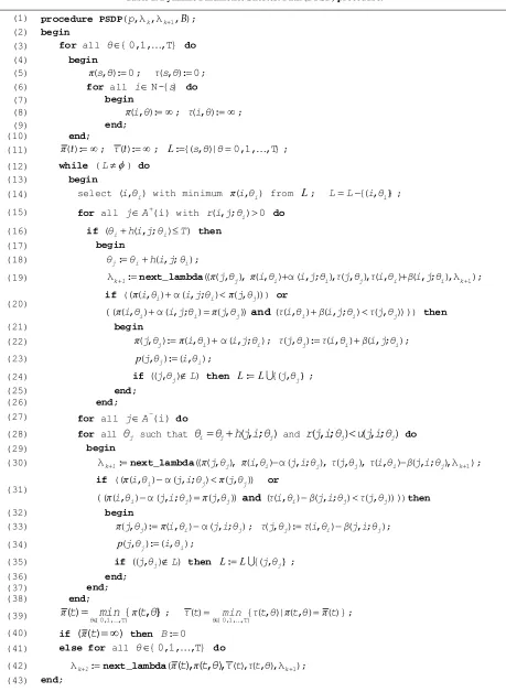
The Pa tric Shortest Dynamic Path (PSDP) pro-cedure is ted in Table 1.

 rame presen

Procedure next_lambda



π1

       

i ,π2 i ,1 i ,2 i



pre-sented in Table 2, returns the value of the parame

ear parametric cost functions ter up to which one of the two lin

of λ remains minimum. The two linear parametric functions to be compared, regarding the arguments of the function, are

 



  

Theorem 2: The complexity of Dynamic Parametric Sh

1 1

π i  λ λ k  i and

 







  

 i .

2 2

π i λ λ_k

ortest Path (DPSP) procedure is





.

Proof: The algorithm performs iterations (se

2

O nmT

 

O nT

lections) and in each of the iterations

 

T arcs are explored (which corresponds to the num of rcs in the time-space network). Hence, the total complexity of the (DPSP) procedure is

O m

ber a



2



O nmT .□

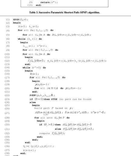
4.2. Successive Parametric Shortest Path

ach successive shortest path algorithm for

the p

Algorithm

step of the E

the bi-criteria minimum cost dynamic flow problem will repeatedly perform the following operations:

i) Compute a parametric shortest dynamic path P from the source node to the sink node;

ii) Find the residual capacity r P

 

of the minimum cost path;

iii) Augment the flow along arametric shortest dynamic path and update the residual network.

For a given value λ_k of the parameter, the algorithm computes the values of ht e parametric costs k



i j, ;



















1 , ; k 2 , ; 1 , ;

c i j c i j c i j

 λ   for λ λ _k

and the slopes of the parametric cost functions



i j, ;



c i j2



, ;



c i j1



, ;



     

for all arcs in the time-dependent residual network. Then the algorithm successively finds parametric shortest dy-namic paths and increases the flow until the value of the dynamic flow for the time horizon T equals the total deficit of all sink node-time pairs, . In each of the it-erations, the value of the parameter by which the para-metric shortest dynamic path remains minimal is com-puted and then the algorithm reiterates with this new value of the parameter. The algorithm will terminate when the value of the parameter becomes equal to 1. The Successive Parametric Shortest Path (SPSP) algorithm is presented in Table 3.

Theorem 3: The Successive Parametric Shortest Path (SPSP) algorithm computes correctly a bi-criteria mini-mum cost dynamic flow for a given time horizon T.

Proof: The consecutive λk values are computed as the closest values of the parameter for which the order of the parametric linear cost functions do not reverse, i.e. do not have crossing points within the interval



λ λk, k₁



. Since for a λ_k value, the flow is augmented along suc-cessive shortest paths, the correctness of the algorithm results from the classical (non-parametric) algorithm. For consecutive λ_k values of the parameter, the proof re-sults directly from Lemma 3.□

122

[image:7.595.67.526.94.722.2]

hor st Path (DPSP) procedure. Table 1. Dynamic Parametric S

(1) procedure PSDP

te

) , λ , λ ,

(p k k1 B; (2) begin

(3) for all θ{0,1,,T} do

(4) begin

(5) π(s,θ):0; τ(s,θ):0; (6) for all iN-{s} do

(7) begin

(8) π(i,θ):; τ(i,θ):;

(9) end;

(10) end;

(11) π(t):; τ(t):; L:{(s,θ)|θ0,1,,T}; (12) while (L) do

(13) begin

(14) select (i,θ_i) with minimum π(i,θ_i) from L; LL{(i,θ_i)}; (15) for all jA(i) with r(i,j;θ_i)0 do

(16) if (θ_ih(i,j;θ_i)T) then

(17) begin

(18) θj:θih(i,j;θi);

(19) λk1:next_lambda((π(j,θj),π(i,θi)α(i,j;θi),τ(j,θj),τ(i,θi)β(i,j;θi),λk1);

(20) if ((π(i,θi)α(i,j;θi)π(j,θj))) or

)) ) , ( ) ; , ( ) , ( ( ) ) , ( ) ; , α( ) , (

((πiθ_i  ijθ_i πjθ_j and τiθ_i βijθ_i τjθ_j ) then

(21) begin

(22) π(j,θ_j):π(i,θ_i)α(i,j;θ_i); τ(j,θ_j):τ(i,θ_i)β(i,j;θ_i); (23) p(j,θj):(i,θi);

(24) if ((j,θ_j)L) then L:L{(j,θ_j)};

(25) end;

(26) end;

(27) for all jA(i) do

(28) for all θj such that θi θjh(j,i;θj) and r(j,i;θj)u(j,i;θj)do

(29) begin

(30) λk1:next_lambda((π(j,θj),π(i,θi)α(j,i;θj),τ(j,θj),τ(i,θi)β(j,i;θj),λk1);

(31) if ((π(i,θi)α(j,i;θj)π(j,θj)) or

)) ) , ( ) ; , ( ) , ( ( ) ) , ( ) ; , α( ) , (

((πiθi  jiθj πjθj and τiθi βjiθj τjθj )then

(32) begin

(33) π(j,θj):π(i,θi)α(j,i;θj); τ(j,θj):τ(i,θi)β(j,i;θj); (34) p(j,θ_j):(i,θ_i);

(35) if ((j,θ_j)L) then L:L{(j,θ_j)};

(36) end;

(37) end;

(38) end;

(39) π(t)_θ{0,min_1,,T}{π(t,θ)}; τ(t)_θ{0,min_1,,T}{τ(t,θ)|π(t,θ)π(t)}; (40) if (π(t)) then B:0

(41) else for all θ{0,1,,T} do

[image:8.595.153.444.89.224.2]

Table 2. Procedure next_lambda.

(1) procedure next_lambda(π1(i),π2(i),τ1(i),τ2(i),λk₁);

(2) begin

(3) λ":λk1;

(4) if (τ₂(i)-τ₁(i))0 then

(5) begin

(6) λ':λk(π1(i)-π2(i))/(τ2(i)-τ1(i));

(7) if ((λ'λk) and (λ'λk1)) then λ":λ';

(8) end;

(9) return(λ");

[image:8.595.84.518.199.714.2]

(10) end;

Table 3. Successive Parametric Shortest Path (SPSP) algorithm.

(1) SPSP(G,v); (2) begin

(3) k:0; λ_k:0;

(4) for all θ{0,1,,T} do

(5) for all (i,j)A do β(i,j;θ):c₂(i,j;θ)-c₁(i,j;θ); (6) while (λ_k1) do

(7) begin

(8) λk1:1; v':v;

(9) for all θ{0,1,,T} do

(10) for all (i,j)A do

(11) begin

(12) fk(i,j;θ):0; αk(i,j;θ)c1(i,j;θ)λk(c2(i,j;θ)c1(i,j;θ));

(13) end;

(14) while (v'0) do

(15) begin

(16) B:1;

(17) for all θ{0,1,,T} do

(18) begin

(19) p(s,θ):0;

(20) for all iN-{s} do p(i,θ):1; (21) end;

(22) PSDP(p,λ_k,λ_k1,B);

(23) if (B0)then STOP (no path can be found)

(24) else

(25) begin

(26) build path P based on p;

(27) r(P):₍min_i,j)P{r(i,j;θi)}; δ:min{v',r(P)}; v':v'-δ;

(28) for all arcs (i,j)P do

(29) begin

(30) if (θ_jθ_i)then r(i,j;θ_i):r(i,j;θ_i)-δ

(31) else r(j,i;θ_j):r(j,i;θ_j)δ;

(32) compute fk(i,j;θi);

(33) end;

(34) end;

(35) end;

(36) Yk:{(y1(fk),y2(fk))};

124

k

λ

term maxi

values, and each problem leads (for the non-degen-erate case) to a new efficient solution. The algorithm

inates when the value of the parameter reaches to the mum value of the unit interval. Starting with λk0 for k0 and ending when λk 1 for kK , the

K

performs steps

linear segments between two consecutive efficient ex-treme points.

Theorem 4: The complexity of the Successive Para-metric Shortest Path (SPSP) algorithm for computing the

t of efficient extreme points in the decision space is

For the labelling operation and computing pa-rametric costs, all arcs at all times have to be examined, so the running time is . Updating the residual networks after augm ow also requires a

run-ning time of ost

algorithm K corresponding to the

se



2



O K nmT v . Proof:

 

O mT

enting the fl . Since at m

 

O mT  augmentations

are done by the algorithm, procedure DPSP is called  times for every λk

trem

value of th com

e eter. Hence efficient ex e point is

param puted in

an

 

O mT

onseque segments be-

+ ntly,

 

O mT +

for the K





2

O nmT

steps corresp

 ,

on

i.e. 

ding to





2

T

linear

O nm

the K

. C

tween two consecutive efficient extreme points, the total

complexity of the SPSP algorithm is _{O K nmT}



_ 2_



_.

rk presented in 3

□

Fig-5. Example

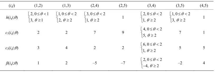
In the discrete-time dynamic netwo

ure 1(a), the problem is to send  units of flo rce node s (nod

e horizon wh acity) of all ar

w at e 1) ich is cs ar minimum bi-criteria cost from th

to the sink node t (node 5) with

set to T = 4. The upper bounds ( e set to

e sou in a tim

cap



, ;



: 2

u i j  , 

 

i j, A

osts are

,   0,1, 2,3 sented in Table







, 4



4. and the t s and c

lope ransit time pre



, ;j



2 , ;

i j c i

   

In the initialisation step, the s





1 , ; c i j 

puted (as pr

of the parametric costs esented in Table 4) an corresponding initial value of th

functions are c for k0 and e parameter 0

om-th

0

d, e



λ ,









0 i j, ; : c i j1 , ;

  

m for the so 

is initialised at all ti nodes except

are set. Th e values to urce node,

e predecessor ve

 

, : 1 p i   fo r which

ctor r all fo p s

 

, is

sed to set to zero, and procedure PSDP

Iteration 1: The distance labe is called.

ls are initiali

 

π 1, : 0 for  



0,1, , T





and the set L of can-didate nodes is set to L:



1,0 , 1

 

      



ode-time pair, (1,0

, .

) is removed from the 1 , 1, 2 , 1,3 , 1, 4 The selected n

[image:9.595.101.500.373.526.2]

Figure 1. (a) The dynamic network G considered for exemplifying how the Successive Parametric Shortest Path (SPSP) algorithm works; (b) The set of all non-dominated points which lie on the efficient boundary in the objective space for the bi-criteria minimum cost dynamic flow problem in network G .

Table 4. Transit times and costs on arcs for the dynamic network in Figure 1.

(i,j) (1,2) (1,3) (2,4) (2,5) (3,4) (3,5) (4,5)

2, 0 1

3, 1

 

  

 _



1, 0 2

2, 2

 

  

 _



3, 0 2

1, 2

 

  

 _

 1

2, 0 2

1, 2

 

  

 _



1, 0 2

3, 2

 

  

 _

 1

h(i,j;)

c1(i,j;) 2 2 7 9

4, 0 2

5, 2

 

  

 _

 7 1

c2(i,j;) 3 4 2 2

6, 0 2

1, 2

 

  

 _

 5 5

β(i,j;) 1 2 –5 –7

4, 2

2, 0  2 

 

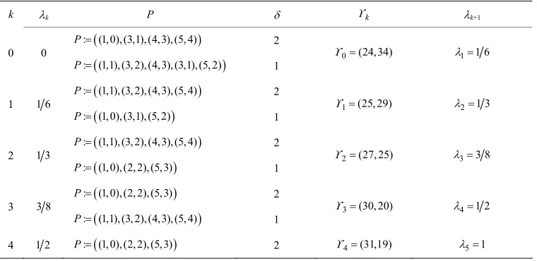
[image:9.595.96.503.587.724.2]

[image:10.595.110.490.101.286.2]

test ath (SPSP) algorithm on the dynamic network in Figure 1. Table 5. The steps performed by Successive Parametric Shor

k k P

P

 k k+1

 

: (1, 0), (3,1),(4,3), (5, 4)

P 2

0 0

 

: (1,1),(3, 2),(4,3),(3,1),(5, 2)

P 1 0(24,34) 11 6

 

: (1,1), (3, 2), (4,3), (5, 4)

P 1

2 1 6

 

: (1,0),(3,1),(5, 2)

P 1 1(25, 29) 21 3

 

: (1,1), (3, 2), (4,3), (5, 4)

P 2

2 1 3

 

: (1,0),(2, 2),(5,3)

P 1 2(27, 25) 33 8

 ), (2, 2), (5,3) 3

: (1, 0

P 2

3 8

 

: (1,1),(3, 2),(4,3),(5, 4)

P 1 3(30, 20) 41 2

4 1 2 P: (1, 0), (2, 2), (5,3)  2 4(31,19) 51

d, ward a d (1,3) at time 0

set L an for the for rcs (1,2) an

  , node-time pairs (2,2) and (3,1) are added to the set L, labelled as: π(2, 2) : 2 , (2, 2) : 1 , π(3,1) : 2 ,

(3,1) : 2

  and p(2, 2) : (1,0) , p(3,1) : ( . ,1) is rem

(1,3) at time

1,0) are set oved from the

1 xt no

for th Then t

set L

he ne and,

de-time pair, (1

e forward arc  , the t L, labelled e pair

node-tim as: π(3

(3,2) is are adde (3, 2) : 2

d to the se , 2) : 2 ,  

) at time and ,2

(3, 2) :

p 

1

(1,1). Since for the arc (1 

will be ) to the si me

time values:

, the transit time no path which

nk node within thing will happen for

2,3, 4





1 1 

e node horizon 1, 2;   h e rc 1 T

e node at all th 3 4   there

-time pair (2,4 = 4. The sa

e other

h

connects t the tim

the sou   .

in increasing bels, is now oved and, for

me 2

Since the ordere

: ( L  the fo

set of candidate nod rresponding



3, 2)



, the first

2,4) and (

e-time pairs, distance la one is rem

2,5) at ti d of 2, 2) rwar thei , (3,1) d r co , (

arcs (  ,

o the set L node-time pairs (4,3) and (5,3) are added t

and labelled as: π(4,3) : 9 , (4,3) : 4, π(5,3) : 11 and (5,3) : 6. The predecessor nodes are set to

(4,3) : (2, 2)

p  and p(5,3) : (2, 2) . Starting from node 3 at time 1

e pair (

, i.e. from th 5,2)

e node-time pair (3,1), the is labelled as π(5, 2) : 9

node-tim  ,

(5,3) : 0

 

,3), a since

nd p(5, 2) : ) 0 (3,1) (3,

(3,1  . As f

;1) 6

or the node-time pair (4 π  4  and π(4,3) 9 , the new label is set to π(4,3) 6 , (4,3) : 4 and the predecessor node is p(4,3) :(3,1) instea

(2, 2)

d of the pre-viously stated value p(4,3) : . Proc

ling node-tim

edure next_ e pair (4,3), lambda

com , in putes the

voked for relabe value λ' : 0 (6 

ter than λ

ext value

9) 4 4) 3

   

0

 and smalle he parameter is

8 wh

set ich r than

to proves to

11

λ

be grea 0

at the n

so th of t

1 k λ Sim 1 : λ ilarly, 3 8. startin 

g from node 3 at time  2, i.e.

from the node-time pair (3,2), since π(3, 2)0(3, 4; 2)

7

 and π(4,3) 6 , the node-time pair (4,3) keeps its tated ure next_lambda, still computes the value

previously s label but proced

' : 0 (6 7) ( 2 4) 1 6     

λ

is greater than 0 0

which 

λ and smaller than λ13 8 so that the next value of the parameter is set to λ: 1 6 . Finally, for the forward arc (4,5) at time 3, the

-tim is labelled as

node e pair (5,4) π(5, 2) :7 , (5,3) : 8

  and p(5,4) : (4,3) is set. inimum puted as: Since the set L is em

sink node at all time

pty, the m values is com

label of the



(5, 4)



,

π(5) :min π(5,0),π(5,1),π(5, 2),π(5,3),π i.e.



, 7



7 and

π(5) : min  , ,9,11  (5) : 8

pute the . com Procedure , consecutively will values

next_lambda ' : 1 4

λ and λ' : 3 14 , both b

than th f

eing greater e previously computed value o λ1

h

: 1 6 . e shortest path Based on the predecessor vector, t





: (1, 0), (3,1) , 4)

P  , (4,3), (5 is built and its residual capacity r P

 

: 2 is computed. The flow is augmented with  : min



v r P',

 



min 3, 2 2

 

 units along this path, the resi ork is

and the updated e value dual netw

xcess

corresp '

ondingly updated  is set to ' : 3 2 1   . Since ' 0 , the algorithm reiterates in th

residu etwor the sh ath

e updated al n k finding ortest p



)



: , 2),(4,3),(3,1),(5, 2 P  (1,1),(3

with r P

 

: 2 , : m in 1, 2

 

1 and ' : 0 , which ution makes the algorithm to stop. The first efficient sol

0

f in the the path

decision space sends two units of flow along



)



: P  along th (1,0),(3,1 e path

),(4,3),(5, 4 and one unit of

flow



),(3,1),(5, 2)



int in th : (1,1),(3,

domina d (24, 34) 2),( ex 4 . trem e ,3 P ing is Y0 The correspond

space

te e po

objective  .

1

126

of flow along t pat and

one unit of flow alo with the extre e point

he h P:



(1,1), (3, 2) 4,3),(5, 4)



ng the path P: (1, 0), (3,1), (5,

in the objective space , (



2)



, 1

Y

m 

(25, 29), and 2: 1 3.

ed by the algorithm are describe space with the non-do i ted in Figure 1(b).

gnanti and J. Orlin, “Network Flows. s and Applications,” Pren e Hall, , New Jersey, 1993.

of Dynamic Network , Vol. 1, No.1, 1 

steps perform nd the objective e points is prese

R. Ahuja, T. Ma y, Algorithm Englewood Cliffs J. A. Aronson, “A Survey

Annals of Operations Research

λ

The Table 5 a extrem

6. References

[1] Theor

[2]

d in nated

Inc.

Flows,” 989, pp. , m n

tic

1-66. doi:10.1007/BF02216922

[3] W.

T

agem

Chin

Powell, P. Jaillet and A. Odoni, “Stochastic

ooks in Operations Research and e, Chapter 3, North Holland, A

Kaw

on & a, 2009, pp.

453-I. Chabini and M. Abou-Zeid, “T ost Flow Problem in Capacitated Dynamic Networks,” Annual Meeting of the Transportation Research Board, Wash-ington, D.C., 20 . 1-30.

E. Nasrabadi and S. M. Hashemi, “Minimum Cost Time- Varying Network Flow Problems,” Optimization Methods and Software, V , No. 3, 2010, pp. 429-447.

and

Man namic Networks and Routing,” In: Ball, M. O., Magnanti,

. L., Monma, C. L. and Nemhauser G. L., Ed., Network

Routing, Handb

-ent Scienc msterdam,

The Netherlands, Vol. 8, 1995, pp. 141-295.

[4] N. Kamiyama, A. Takizawa, N. Katoh and Y. abata, “Evaluation of Capacities of Refuges in Urban Areas by Using Dynamic Network Flows,” Proceedings of the Eighth International Symposium Operations Research and Its Applications, ORSC APORC, Zhangjiajie,

460.

[5] he Minimum C

03, pp [6]

ol. 25

doi:10.1080/10556780903239121

H. Lee and S. Pulat, “Bicriteria Network Flow Problems: Continuous Cas European Journal of Operational Re-search, Vol. 51, No. 1, 1991, pp. 119-126.

[7]

e,”

doi:10.1016/0377-2217(91)90151-K

S. Gass and T. S y, “The Computational Algorithm for the Parametric Objective Function,” Naval Research Lo-gistics Quarterly , No. 1-2, 1955, pp. 39-45.

[8] aat

, Vol. 1

doi:10.1002/nav.3800020106

[9] A. M. Geoffrion, “Solving Bicriterion Mathematical Pro-grams,” Operations Research, Vol. 15, No. 1, 1967, pp. 39-54. doi:10.1287/opre.15.1.39

d K. ransporta

1979, p [10] Y. P. Aneja an P. Nair, “Bicriteria T tion

Problem,” Management Science, Vol. 25, No. 1, p. 73-78. doi:10.1287/mnsc.25.1.73

[11] A. Skriver, “A Classification of Bicriterion h

ific Journal

Shortest Pat (BSP) Algorithms,” Asia-Pac of Operational

ying Network

Research, No. 17, 2000, pp. 199-212. [12] X. Cai, D. Sha and C. Wong, “Time-Var