5) In this problem we explore a slight change to the standard quadratic optimal controller.

ECE-320: Linear Control Systems Homework 4

Due: Tuesday September 29 at the beginning of class

Quiz #4 on Tuesday September 29, Exam #1 on October 1

1) For a system with plant

3 ( ) ( 1) p s G s s s + = −

a) Show that the quadratic optimal closed loop transfer function for q=100 is

0 2 10( 3) ( ) 12.7 30 s G s s s + = + +

and the controller is

10( 1) ( ) 2.7 c s G s s − = +

b) Show that with this controller, the steady state errors for unit step and unit ramp inputs are 0.0 and 0.09, respectively.

2) For a system with plant

1 ( ) ( 2) p s G s s s − = −

a) Show that the quadratic optimal closed loop transfer function for q=100is

0 2 10( 1) ( ) 11.1 10 s G s s s − − = + +

and the controller is

10 20 ( ) 21.14 c s G s s − + = +

3) Assume we have the following system

( )

p

G s

( )

c

G s

+

-where ( ) 1 2

p

G s s

=

+ . We want to design a model matching controller so that • the closed loop system is a second order

• the state error for a step input is zero

• the settling time of the closed loop system is 3 seconds

• the percent overshoot of the closed loop system is 20%

. You are to determine the closed loop transfer function and then the controller to meet these specifications.

Ans. ( ) 8.53( 2) ( 2.66)

c

s G s

s s

+ =

+

4) Assume we have the following system

( )

p

G s

( )

c

G s

+

-where ( ) 1 2

p

G s s

=

+ . We want to design a model matching controller so that • the closed loop system is a second order

• the steady state error for a step input is zero

• the bandwidth of the closed loop system is 2 Hz.

Luckily I have an uncle who sells good poles cheap, so I obtained a pole at 10− π rad/sec for your system. You are to determine the closed loop transfer function (i.e., find the other pole and the numerator) and then the controller to meet these specifications. (Hint: Read Chapter 7 of the notes!, Ans.

2

40 ( 2)

( )

( 14 )

c

s G s

s s

π π + =

5) In this problem we explore a slight change to the standard quadratic optimal controller. We assume we have the following system, with prefilter G_pf , plant G s_p( ) and controller

( )

c

G s

pf

G

_{( )}

p

G s

( )

c

G s

+

-a) Assume the plant is

200 ( )

10

p

G s s

= +

and we want to design a quadratic optimal controller with q=0.001. Show that

0

3.381 0.0169( 10)

( ) ( ) 3.5

11.832 c 8.451 p

s

G s G s G

s s f

+

= =

+ + =

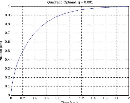
in order to have a steady state error for a unit step of zero.

Simulate the system with a unit step input. Your results should look like that in Figure 1. Turn in this plot.

b) Assume we utilize the quadratic optimal algorithm as above to determine, but rather than utilizing a prefilter, we scale the closed loop transfer function so t

0( ) G s

hatG₀(0)=1 Show that we then get

0.05916( 10) ( )

c

s G s

s

+

= and G_pf =1

Simulate the system using this controller and prefilter with a unit step input. Your results should look like that in Figure 1.

Note that we are not guaranteed we will be able to get an implementable transfer function if we scale G₀( )s so that G₀(0)=1, but if we can, we get a type 1 system and there is no scaling outside the of the feedback loop (Gpf =1 )! Why do we care? See part

c, d, and e below.

c) Assume that despite your best efforts, you did not get the model for the plant exactly correct, and instead, the correct transfer function for the plant is

190 ( )

12

p

G s s

= +

d) Now simulate this system (plant from part c) with a unit step input using the controller and prefilter from part (b). You should get results like those in Figure 3. Turn in your graph.

e) Assume that your fool of a lab partner copied down the numbers incorrectly, and the plant is more accurately modeled as

100 ( )

20

p

G s s

= +

Show (analytically) that the steady state error for the original system for a step input with amplitude A is 0.68A, while the corresponding steady state error for the type 1 system is still 0. Simulate this plant using the original control system (part a) and the modified control system (part b). You should get results like those in Figures 4 and 5. Turn in your graphs.

The moral of this problem is that, if we can, we are usually better off if we do not depend on anything outside the feedback loop! Type 1 systems can help alot with modeling errors if we want a zero position error. However, it may take a long time to reach the zero position error.

6) Consider the following control system:

( )

c

G s

+

-We are going to use quadratic optimal control to determine the closed loop transfer function and the controller . For quadratic optimal control we determine the closed loop transfer function to minimize

( )

o

G s G s_c( )

( )s

o

G

2 2 0 ( ( ) ( )) ( ) J =

∫

a) Determine the value of q so that the (2%) settling time of the system is (approximately) 1 second. Hint: Solve for in terms of q, then figure out what q should be to meet the settling time requirements.

( )

o

G s

b) Determine the controllerG_c( )s .

Figure1. The step response for the correct plant and original controller (Problem 5, part a)

0 0.1 0.2 0.3 0.4 0.5 0.6 0.7 0.8 0.9 1 0

0.1 0.2 0.3 0.4 0.5 0.6 0.7 0.8 0.9 1

Time (sec)

P

os

it

ion (

c

m

)

Quadratic Optimal, q = 0.001

Figure 2. The step response for the new plant and the original controller (Problem 5, part c)

0 0.1 0.2 0.3 0.4 0.5 0.6 0.7 0.8 0.9 1 0

0.1 0.2 0.3 0.4 0.5 0.6 0.7 0.8 0.9

Time (sec)

P

os

it

ion (

c

m

)

Figure 3. Step response of the new plant with the type 1 controller (Problem 5, part d)

0 0.1 0.2 0.3 0.4 0.5 0.6 0.7 0.8 0.9 1 0

0.1 0.2 0.3 0.4 0.5 0.6 0.7 0.8 0.9 1

Time (sec)

P

os

it

ion (

c

m

)

Quadratic Optimal, q = 0.001

Figure 4. Step response of the new plant with the original controller (Problem 2, part e)

0 0.1 0.2 0.3 0.4 0.5 0.6 0.7 0.8 0.9 1 0

0.05 0.1 0.15 0.2 0.25 0.3 0.35

Time (sec)

P

os

it

ion (

c

m

)

Figure 5. Step response of the new plant with the type 1 controller (Problem 5, part e)

0 0.2 0.4 0.6 0.8 1 1.2 1.4 1.6 1.8 2 0

0.1 0.2 0.3 0.4 0.5 0.6 0.7 0.8 0.9 1

Time (sec)

Po

s

iti

o

n

(

c

m

)

Quadratic Optimal, q = 0.001

Note that we trade off zero position error for a longer settling time.

Preparation for Lab 4.

Download the file solve_quadratic.m from the class website. The input arguments to this function are (1) the transfer function of the plant Gp, and (2) the value of q. The routine returns the optimal closed loop transfer function Go(s). To use this function with problem 1 we would type something like the following:

Gp = tf([1 3],[1 -1 0]); q = 100;

Go = solve_quadratic(Gp,q) Gc = mineral(Go/(Gp*(1-Go)))

7) Check your answers to problems 1 and 2 and be sure you understand how to use this function.

8) Modify closedloop_driver.m to implement a quadratic optimal controller. Be organized and neat! You will need to be able to figure out what you have done later! You should have one section of code for determining the plant, one section of code for finding the controller, one section of code for

determining the prefilter, and one section of code for plotting the results! Each lab partner should do this separately (though you can help each other).

Comment out any controller you currently have (don’t delete!), and implement the quadratic optimal controller as shown above. (Your Gp will come from your model.)

Determine the value of the prefilter so the steady state error for a unit step is 0. This should be coded in Matlab based on the closed loop transfer function. Do not just use a number here (unless it’s a 1).

For ECP-210 systems assume the input is 1 cm, for ECP-205 system assume the input is 15 degrees (be sure to convert to radians for the input, but plot the output in degrees), Plot the appropriate step

responses for q=0.001, q = 0.01, and q = 0.1. How dose changing q affect the response and the maximum control effort?