ece300 lab05 fourier coef

(1)

ECE 300 Signals and Systems Fall 2007

Measurement of Fourier Coefficients

Lab 05

by Bruce A. Black with some tweaking by others

Objectives

• To measure the Fourier coefficients of several waveforms and compare the measured values with theoretical values.

• To become acquainted with the Agilent E4402B Spectrum Analyzer.

Equipment

Agilent E4402B Spectrum Analyzer Agilent Function Generator

Oscilloscope BNC T-Connector

Background

Recently we learned to calculate the spectrum of a periodic signal by using the Fourier series. We have in our lab spectrum analyzers that can display the spectrum of a signal in pseudo- real time. The Agilent E4402B Spectrum Analyzer (SA) can be used to view the power spectrum of any signal of frequency up to 3 GHz. The SA displays a “one-sided spectrum” in decibels (dBs) versus frequency. In lab we will observe the spectra of sinusoids, square and triangle waves, and pulse trains, but first we must learn how to convert the Fourier series coefficients that we

calculate to the dB values displayed by the spectrum analyzer.

Recall that any periodic signal x t

( )

can be written as

( )

2 0

0 0

, where 1

j kf t k k

x t a e π f

∞

=−∞

=

∑

= T .

Writing out a few terms gives

( )

0 0 0 0

0 0 0

2 1 1 2

2 2 2 2 2 2

2 1 0 1 2

2 2 2 2 2 2

2 1 0 1 2

j f t j f t j f t j f t

j a j a j a j a

x t a e a e a a e a e

a e e a e e a a e e a e e

π π π π

− − − − − − − − = + + + + + + = + ( + ( + + ( + ( + " "

" 0 "

k

(1)

where we have used the fact that a₋_k =a∗ whenever x t

( )

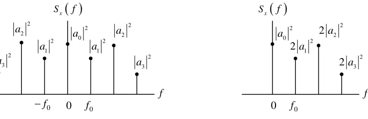
is real-valued. Notice that, aside from , the terms come in pairs (actually, complex conjugate pairs). We can combine each positive-frequency term with its matching negative positive-frequency term to obtain

0 a

(2)

to be a_k 2 (and corresponds most directly with equation (1)). The corresponding one-sided

power spectrum is shown in Fig. 2. To make the one-sided spectrum, the powers associated with complex exponentials at frequencies kf₀ and −kf₀ are added. The result, representing the

average power in the sinusoid 2 a_k cos 2

(

πf t_k +(a_k

)

, is shown at frequency (and corresponds most directly with equation

[image:2.612.106.476.178.298.2]

0 kf (2)).

( )

x S f f 0 f 0 f − 2 0 a 2 1 a 2 1 a 2 2 a 2 2 a 2 3 a 2 3 a 0

( )

x S f f 0 f 2 0 a 2 1 2a 2 2 2a 2 3 2 a 0

Figure 1: Two-Sided Power Spectrum Figure 2: One-Sided Power Spectrum

The SA displays a one-sided spectrum as shown in Fig. 2, but instead of showing the value of

2

2ak at each frequency, the spectrum analyzer shows average power in decibels with respect to

a one millivolt RMS reference. For the sinusoid at frequency , the average power in decibels is given by

0 kf

10

10 log k k dB ref P P P = ,

where the power Pk represents the power spectrum coefficient 2

2a_k , and the power Pref is the

average power delivered to a one-ohm resistor by a one millivolt RMS sinusoid. We have

(

)

2

10 log dBmV 0.001

k k dBmV

a

P = .

The units “dBmV” indicate that the reference for the decibels is a one millivolt RMS sinusoid.*

Note: The spectrum analyzer will not display the DC term a₀ 2 even when one is present in the signal. Instead it displays a large spike at zero frequency allowing for easy location of DC on the display. Also, because it is showing a power spectrum, the spectrum analyzer does not measure or display the phase angles (a_k.

[image:2.612.93.274.179.298.2]

(3)

Procedure

Read the documents “SA_hints_E4402B” and “Reading_SA_Display_E4402B”, both available on the class webpage.

The waveforms we will be analyzing, each having zero DC offset, are:

a) x t₁

( )

=0.1cos 2 100 10

(

π × 3t

)

V

b) x₂

( )

t is a square wave of period 10 μs and peak-to-peak amplitude 0.2 V.

c) x t₃

( )

is a triangle wave of period 10 μs and peak-to-peak amplitude 0.2 V.

Just to be sure there is no confusion regarding the waveforms, they are displayed below.

a) b)

c)

Getting Ready

(4)

Calibrate the Spectrum Analyzer

Calibrate the spectrum analyzer as described in the document SA_hints_E4402B.

Measuring the Spectrum

1. Use the function generator to generate a sinusoid of frequency 100 kHz and (open circuit) amplitude 0.1 V (waveform a). Use the oscilloscope to verify the amplitude**. Now observe the signal power spectrum on the spectrum analyzer. Measure the power level and frequency. Record your measurements in the table on the final page of this lab.

2. Informally vary the frequency and the amplitude of the sinusoid and observe how the spectrum analyzer display changes.

3. Use the function generator to generate a square wave of period 10 μs and peak-to-peak amplitude 0.2 V (waveform b). Using the spectrum analyzer, measure the level of the first nine harmonics. Record your measurements in the table on the final page of this lab.

4. Use the function generator to generate a triangle wave of period 10 μs and peak-to-peak amplitude 0.2 V (waveform c). Use the spectrum analyzer to measure the level of the first nine harmonics. Record your measurements in the table on the final page of this lab.

** Note concerning Agilent FG amplitude readings.

(5)

Measurement of Fourier Coefficients-Instructor Verification Sheet

Name ___________________________________________ Date of Lab: __________________

Record your procedure for using the spectrum analyzer in the space below. How should the output of the signal generator be set? Is the signal measured on the oscilloscope the size predicted by the signal generator?

Summary of Results for Waveform 1

Harmonic

Prelab Predicted Power (dBmV)

Measured Power

(dBmV) Error (dBmV) Frequency (kHz) 1 37.0

Harmonic

Measured Power

2 ---

3 29.5

4 ---

(6)

Harmonic

Measured Power

2 ---

3 16.1

4 ---

5 7.2

6 ---

7 1.4

8 ---