plant . For example, the settling time for a step input may be longer than we would like,

ECE-205 Lab 7

Feedback Control Systems

Overview

In this lab you will be introduced to the idea of feedback control. We will simulate first and second order systems in a feedback loop with a controller. Next week we will build some of these systems so you can see how we can relate the math and the block diagrams to a real system.

PART I : Feedback Systems

Sometimes we have a system and it responds in a way we wish to modify. In control systems we often refer to such as system as the plant. For example, the settling time for a step input may be longer than we would like, the overshoot may be larger than we want, or we want the output of our system to match the input of our system (if we put a step of amplitude one into the system, we want the output of the system to eventually equal one). While it is sometimes possible to directly modify the systems to achieve what we want, such as changing the values of circuit elements to change the time constants, sometimes we really cannot do that and have to just deal with the plant (our original system) and try to modify its behavior in another way. This is the main focus of control systems, which we will investigate a little bit here.

We will assume that we designate the transfer function of our plant as G sp( ). Hence, for our usual first and

second order systems we have

2 2 2 ( ) , ( ) 1 2 n p p n n K K

G s G s

s s s



  

 

  

In order to change the behavior of the plant, we are going to do two things, both of which are depicted in Figure 1. The first of these is to provide some feedback so we can compare the input and output of the system. This difference is called the error signal, and it is just the difference between the input and the output. In the diagram the error signal is depicted as E s( ), and it is the difference between the reference signal R s( ) and the output signal Y s( ),E s( )R s( )Y s( ). In most control systems we want the output to equal the reference signal. The second thing we will do is to include a new system called a controller, that we depict by the transfer function,

( ) c

G s , that operates on the error signal and produces a new signal, the control effort U s( ), which is the input into the plant. Note that the control effort is not the transfer function of the unit step. It is unfortunate that it is conventional to use the same notation for two things, but that’s just the way things are. You will know which is which by the context in which it is used. We will denote the closed loop transfer function for this system as

( ) o

G s , and clearly we have

( ) ( ) ( )

1 G ( ) ( )

c p

o

c p

G s G s G s

s G s

In this lab we will look at three common controllers, a proportional (P) controller, and integral (I) controller, and a proportional plus integral (PI) controller.

For a proportional (P) controller, the signal to the plant, u t( ), is directly proportional to the error signal e t( ) . So we have u t( )k e tp ( ). In the Laplace domain this becomes U s( )k E sp ( ), and the transfer function for the

proportional controller is then ( ) ( ) ( )

c p

U s

G s k

E s

  .

For an integral (I) controller, the signal to the plant is proportional to the integral of the error signal. So we have

0 ( ) ( )

t

i

u t k e



U s E s

s

 , and the transfer function for the integral

controller becomes ( ) ( ) ( ) i c k U s s

E s s

G  

For a proportional plus integral (PI) controller, the input to the plant is proportional to both the error and the

integral of the error (with two scaling factors). We have then

0 ( ) ( ) ( )

t

p i

u t k e t k e



this is

( / )

( )

( ) i ( ) p i ( ) p i p ( )

p

k

k s k s k k

k

E s E s E s E s

s U

s s

s k     

We often just write the transfer function for the PI controller as ( ) ( ) ( ) ( )

c

U s k s z

s

E s s

G   

In what follows we will use these controller types, but you will be told the values of the proportionality constants to use. Again, we will first show you how to simulate the systems in Matlab, then in Simulink.

PART I I: Simulating Feedback Systems

In this part we will show you how to simulate closed loop systems using both Matlab and Simulink. We will be modifying the open loop simulations you did last week. Much of these instructions are already in the file, so just modify it as you need to. At this point your probably should comment out the line sim(‘openloop’), since we will not be using Simulink for a while.

1) Open the Matlab m-file you used last week, and save it under a new file name. Do not just overwrite the existing file! We will use one m-file (which you will e-mail with your memo) for this lab. Be sure you have the command clear variables at the beginning of your Matlab script@

2) Set the variables tau = 0.001 and K = 2.0

3) Enter the transfer function

1 p G K s  

 into Matlab.

4) Enter the final time variable Tf = 0.01 (be sure to use at least one capitol letter so it is not confused with the transfer function command tf).

6) Let’s assume we want a step input with an amplitude of 0.1. There are many ways to generate this, but we will use the following command (note that the input is now r, not x!):

r=0.1*ones(1,length(t));

7) Now we need to make the controller. For our first controller we will use a proportional controller with proportionality constant k_p 0.2. Enter the transfer function into Matlab,

Gc = tf(0.2,1);

8) Next we construct the closed loop transfer function. However, there is one extra command we need to use, and that is minreall. The minreal command removes pole/zero cancellations. Enter the closed loop transfer function into Matlab,

Go = minreal(Gc*Gp/(1+Gc*Gp))

9) To simulate the system, we then use the lsim command as follows:

y = lsim(Go,r,t); % note that the input to the system is now r, not x!!

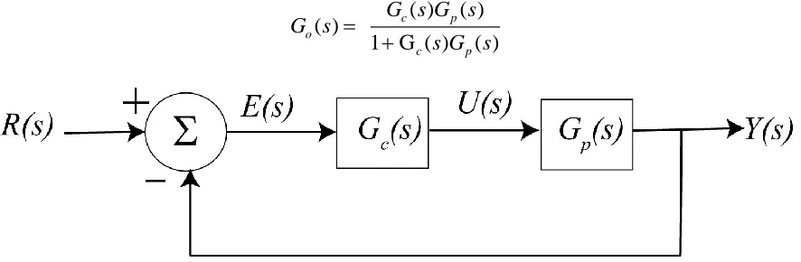
10) Figure 2 shows the open loop response of this system you determined last week. Your closed loop response should look that that shown in Figure 3. (Note that I have really plotted more than one graph in this figure, which you will do shortly.) If you compare these two figures, you should note two things:

 The settling time is much faster for the system with feedback

 The steady state values are different for the two systems, but neither one of them actually matches the reference input signal (the reference signal in this case is 0.1)

You will include Matlab and Simulink Figures of the following in Step 21, so don’t save your graphs to your memo yet.

11) Modify your controller so kp 1 and then kp 5. What do you notice? (write something in your memo

about this!).

12) Now change final time to 0.02 seconds, and simulate the system for the following two integral controllers,

( ) 200

c

G s s

 and G s_c( ) 500

s

 . You should note that the settling time is now larger, but we match the reference

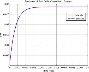
input (the steady state value of the output is 0.1). However, as we increase the proportionality constant the percent overshoot increases. The correct response for the second controller is shown in Figure 4.

13) Now change the final time to 0.00005 seconds (5e-5), and simulate the system for the following two

integral plus proportional controllers, G s_c( ) 100(s 10)

s



 and G s_c( ) 500(s 10)

s



 . Now the settling time is

Figure 2. Open loop response of first order system to a step of amplitude 0.1

Figure 3. Closed loop response of first order system to a step of amplitude 0.1 using a proportional controller with a proportionality constant of 0.2

0 0.001 0.002 0.003 0.004 0.005 0.006 0.007 0.008 0.009 0.01 0

0.02 0.04 0.06 0.08 0.1 0.12 0.14 0.16 0.18 0.2

Time (sec)

y

(t

)

Response of First Order System

Matlab Simulink

0 0.001 0.002 0.003 0.004 0.005 0.006 0.007 0.008 0.009 0.01 0

0.005 0.01 0.015 0.02 0.025 0.03

Time (sec)

y

(t

)

Response of First Order Closed Loop System

Figure 4. Closed loop response of first order system to a step of amplitude 0.1 using the integral controller

500 ( )

c

G s s

 . Note that the steady state output is the same as the reference input.

Figure 5. Closed loop response of first order system to a step of amplitude 0.1 using the proportional plus

0 0.002 0.004 0.006 0.008 0.01 0.012 0.014 0.016 0.018 0.02 0

0.02 0.04 0.06 0.08 0.1 0.12

Time (sec)

y

(t

)

Response of First Order Closed Loop System

Matlab Simulink

0 1 2 3 4 5 6

x 10-5 0

0.01 0.02 0.03 0.04 0.05 0.06 0.07 0.08 0.09 0.1

Time (sec)

y

(t

)

Response of First Order Closed Loop System

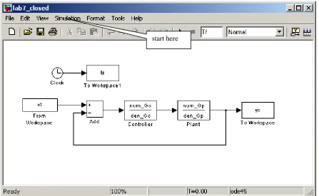
We now want to modify the Simulink, model you derived last week so it will model our closed loop system.

14) Open your Simulink model from last week and save it as closedloop.mdl.

15) Modify your model so it looks like that in Figure 6.

Figure 6. Closed loop Simulink model file.

16) Since we are dealing with small time scales, we will need to modify the maximum default time step in Simulink. Click on Simulation and then Configuration Parameters and set the Maximum Step Size to 1e-6. The next two figures show the basic idea. Save the model file when you are done.

17) We will be using the times and input values from Matlab, so enter the command

rt = [ t’ r’];

into Matlab.

18) We although we already know the numerator and the denominator of the controller transfer function, let’s extract them from the transfer function. We use the command

[num_Gc,den_Gc] = tfdata(Gc,’v’);

19) Run the simulation from the m-file using the command,

sim(‘closedloop’);

20) At this point you have results from both Matlab (t,y) and Simulink (ts, ys). Modify your m-file to plot both of these results on the same graph. Use two different line types and colors, use a grid, label the x-axis etc. so your results look like those in the previous figures 2-4.

21) Repeat steps 11, 12, and 13. Your graphs should show that the Matlab and Simulink results are essentially the same. You need to save all six graphs in your memo.

22) Now you need to modify your m-file so you can plot the results for a second order system with a natural

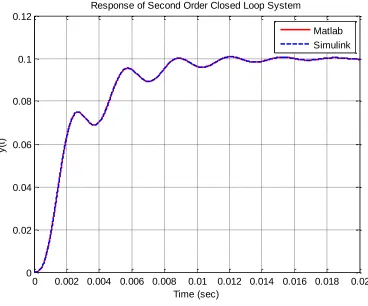
23) Simulate your system (both Matlab and Simulink) for the integral controller G s_c( ) 250

s

 . Your result

should look like that in Figure 7. You need to include your graph in your memo.

Figure 7. Closed loop response of second order system to a step of amplitude 0.1 using the integral controller

( ) 250

c

G s s

 . Note that the steady state output is the same as the reference input.

PART III: Prefilters for Modifying Steady State Values

Sometimes when we use feedback control, we need to be able to adjust the steady state output value. This is very apparent in our first order system when we used a proportional controller. In that case, we were able to significantly change the settling time of the system, but the output did not equal the input. What we need is a proper scaling, and this is usually called a prefilter. Figure 8 shows our basic feedback loop with a prefilter. The prefilter can either be a transfer function or a constant. In this lab we will assume the prefilter is a constant, so G_pf( )s G_pf .The purpose of the prefilter is to take the reference signal and scale it so the input to the system

matches the output of the system.

0 0.002 0.004 0.006 0.008 0.01 0.012 0.014 0.016 0.018 0.02 0

0.02 0.04 0.06 0.08 0.1 0.12

Time (sec)

y

(t

)

Response of Second Order Closed Loop System

Figure 8: Basic feedback control loop with a prefilter.

If the closed loop system has the transfer function,

0

0 ( ) ( )

( )

o

N s s

D G

s



then we want the prefilter to have the value (don’t worry why)

0

0 (0) (0)

pf

D G

N



There are two ways to evaluate a polynomial at zero, but the easiest way to do this is to use the end parameter, as follows:

[num_Go,den_Go] = tfdata(Go,’v’); num_Gpf = den_Go(end);

den_Gpf = num_Go(end);

1) Implement the dynamic prefilter in both your Simulink model and Matlab models. The easiest way to do this is to redefine Go as, Go = Go*num_Gpf/den_Gpf. You do this just after you determine Go.

2) Rerun Part II, number 11 (the first order system), and be sure your steady state output value matches the input value. Include both of your plots in your memo.