8.0 Steady State Frequency Response
Consider the response of two LTI system with transfer functions 1
5 ( )
1 s
H
s =
+
2 2
80 ( )
1.2 10 H s
s s
=
+ +
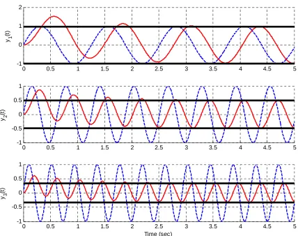
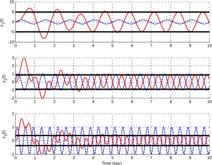
to the inputs x t( )=sin(ω0t u t) ( ) forω0= 5, 10, and 15 radians/sec. Figure 8.1 displays the response of the first system to the three input sinusoids, while Figure 8.2 displays the response of the second system to the three input sinusoids. In both figures, the input sinusoid is displayed as a dashed line and the output is a continuous line. Both figures include heavy solid lines that bound the amplitude of the output sinusoid in steady state. As the figures demonstrate, both of the systems go through some initial transients, and then reach a steady state response. The first system has a pole at -1 and the second system has its poles at approximately −0.6 3± .1j, so the 2% setting times for the two systems are estimated to be 4 and 6.7 seconds which corresponds pretty well with the results in the figures. Once the systems come into steady state, the output of the system has a constant amplitude, and there is a constant relationship between the input signal and the output signal. It is important to note that the settling time for the system is not a function of the frequency of the input, but is a property of the system!
At this point we know how to quickly estimate the settling time of a system based on the poles of the system, and we next want to be able to quickly estimate the steady state output of an asymptotically stable system with a sinusoidal input. In order to do this we first need to review Euler’s identities and write them in a different form than you are used to seeing.
8.1 Euler’s Identity and Other Useful Relationships
The usual form of Euler’s identity is 0
0 0
cos( ) sin( )
j t
t j t
eω = ω + ω
We can also write this as
0
0 0
cos( ) sin( )
t j
t j t
e− ω = ω − ω If we add and subtract these two expressions we get
0 0 0 0
0 0 2 cos( ) 2 sin( )
j t j t
j t j t
e t
e e j
eω ω
ω ω
ω t ω
−
−
+ =
− =
Finally, we get our alternate forms of Euler’s identity 0 0
0 0 0
0 cos( )
2 sin( )
2
j t j t
j t j t
e e
t
e e
t
j
ω ω
ω ω
ω
ω
−
− + =
− =
This form of Euler’s identity is very useful in both this and in later courses.
Figure 8.1. Response of the first system to sinusoids of 5, 10, and 15 radians/sec. The estimated settling time of the system is 4 seconds. The input signal is the dashed line and the output signal is the solid line. The thick solid line bounds the steady state amplitude.
0 0.5 1 1.5 2 2.5 3 3.5 4 4.5 5
-1 0 1 2
y 1
(t
)
0 0.5 1 1.5 2 2.5 3 3.5 4 4.5 5
-1 -0.5 0 0.5 1
y 2
(t
)
0 0.5 1 1.5 2 2.5 3 3.5 4 4.5 5
-1 -0.5 0 0.5 1
y 3
(t
)
Time (sec)
Next, let’s assume our usual case of a proper transfer function that is the ratio of two polynomials,
1
1 1
1
1 1
( )
s
m m
m m
n n
n
b s b s b s b
H s
s a a s a
− −
− −
0 0
+ + + +
=
+ + + +
" "
Since this is proper we have . Let’s also assume that we have a real valued system, so that if the input is a real valued function the output will be a real valued function. This means that all of the coefficients must be real values. To understand this, remember that this transfer function means the input and output are related by the differential equation
m≤n
1
1 1 1 0 1 1 1
1
( ) ( ) ( ) ( ) ( ) ( )
( ) ( )
m m
n m m m m
n n
n n
x x
a a a b
d y t d y t dy t d t d t dx t
0
y t t
dt dt dt dt b dt b dt b
−
− − − −
−
+ + +" + = + + +" + x
Hence, if the input is real and we want the output to be real all of the coefficients must also be real.
[image:2.612.97.525.90.428.2]Figure 8.2. Response of the second system to sinusoids of 5, 10, and 15 radians/sec. The estimated settling time of the system is 6.7 seconds. The input signal is the dashed line and the output signal is the solid line. The thick solid line bounds the steady state amplitude.
0 1 2 3 4 5 6 7 8 9 10
-10 -5 0 5 10
y 1
(t
)
0 1 2 3 4 5 6 7 8 9 10
-2 -1 0 1 2 3
y 2
(t
)
0 1 2 3 4 5 6 7 8 9 10
-1 0 1 2
y 3
(t
)
Time (sec)
Next, let’s assume we want to evaluate the transfer function ats= jω0 and also at 0
s= −jω and if we can relate the two. Remember that as we raise j to increasing powers we cycle through the same four values, i.e., 1
j = j, 2 1
j = − , 3
j = −j, 4 , and 1
j = 5
j = j
so we are right back where we started. To determine what is going on with transfer functions we will look at low order systems and build are way up. Finally, remember that to determine the complex conjugate of a number, you replace j with –j.
[image:3.612.100.525.83.415.2]First Order System:
*
1 0 1 0 0 1 0 0
0 0
0 0 0 0 0
) )
( ) b , ( jb , ( jb (
H s H j H j H j
s a j a
s b
j
b b
a 0)
ω ω
ω ω ω
ω ω − = − + + − + + = + = + =
Second Order System:
2 2
2 1 0 2 0 1 0
0
2 2
1 0 0 1 0 0
2
*
2 0 1 0 0
0 2 0
0 1 0 0
( ) , ( ,
( (
)
) )
b b b jb
H s H j
s a s a ja a
b
s s
jb
H j H j
ja b b a b ω ω ω ω ω ω ω ω ω ω ω + + − + = + − + − − − = = = − − + + + 0 + +
Third Order System:
3 2 3 2
3 2 1 0 3 0 2 0 1 0 0
0
3 2 3 2
2 1 0 0 2 0 1 0 0
3 2
*
3 0 2 0 1 0 0
0 3 2 0
0 2 0 1 0 0
( ) , (
) (
) ,
) (
b b b jb b jb
H s H j
s s a s a j a ja a
jb b jb
H j H j
j a j
s s s b
b a
b a
a
ω ω ω
ω
ω ω ω
ω ω ω
ω ω
ω ω ω
+ + = + + + + + = + − − = + − − + − − − = − − + +
Fourth Order System:
4 3 2 4 3 2
4 3 2 1 0 4 0 3 0 2 0 1 0
0
4 3 2 4 3 2
4 2 1 0 0 0 2 0 1 0 0
4 3 2
*
4 0 3 0 2 0 1 0 0
0 4 3 2 0
0 3 0
3
0 2 0 1 0
)
( ) , ( ,
( ) ( )
b b b b b jb b jb
H s H j
s s s a s a ja a ja a
b jb b jb
H j H j
ja a ja a
s s s s b b
a a
b
ω ω ω ω
ω
ω ω ω ω
ω ω ω ω
ω ω
ω ω ω ω
+ − − = + − + + + + + = + + + + + = − + + − = − + + − − − 0 ) At this point it is pretty straightforward to generalize the relationship H*(jω)=H(−jω . The last thing we need to do is look at representing the transfer function in polar form to determine two important properties of transfer functions for real-valued systems. Assume that we have the complex function written in rectangular form as
(
( ) a ) ( )
z ω = ω + jb ω
where a( )ω and b( )ω are real valued functions. We can write this in polar form as
( ) ( )
( ) ( ) jd | ( ) | j z
z ω =cω e ω = z ω e ( ω
where 2 2 1 ) ( ) ( ) | ( ( ) ( ) ) ( ( tan ( ) a b c b d z a ) | z
ω ω ω ω
ω ω ω ω − = + = ⎛ ⎞ = ⎜ ⎟= ⎝ ⎠ (
Now let’s assume we have a complex valued transfer function H j( ω). We can write this in polar form as
( ) ( ) | ( ) | j H j
H jω = H jω e ( ω
Next, let’s look at H*(jω) and H(−jω) to derive some useful relationships.
* * ( ) ( )
( ) | ( ) | j H j | ( ) | j H j
H jω = H jω e− ( ω = H jω e−( ω
( ) ( )
( ) | ( ) | j H j | ( ) | j H j
H −jω = H −jω e ( −ω = H −jω e ( −ω
Now since we know that for a real valued systemH*(jω)=H(−jω) we can conclude the following useful information:
• |H j( ω) | |= H(−jω)| (the magnitude is an even function of frequency) • −(H j( ω)=(H(−jω)( the phase is an odd function of frequency)
Although we have only shown this to be true for transfer functions that are ratios of polynomials, it is true in general for any transfer function that corresponds to a real valued system. It may also seem a bit odd to talk about negative frequencies, but this is necessary for the mathematics to work out. Often when we plot the frequency response of a system we will plot both negative and positive frequencies, even if we can only
measure the positive frequencies.
With this background, we can now solve our problem.
8.2 Steady State Response to a Periodic Input
Let’s assume we have strictly proper rational transfer function for a real valued , asymptotically stable, system which has distinct poles. The we can represent the transfer function as
n
1 1
1 1 0 1 1
1
1 1 0 1 2
( )
s ( )( )
m m m m
m m m m
n n
n n
b s b s b s b b s b s b s b
H s
s a a s a z p z p z p
− −
− −
− −
+ + + + + + + +
= =
+ + + + − − −
" "
" "
0
( )
Next, assume the input to our system is a cosine with amplitude A, x t( )=Acos(ω0t u t) ( ). We can then use Laplace transforms to determine the output of the system,
2 2
0 0
( ) ( ) ( ) ( ) ( )
( )(
As As
Y s H s X s H s H s
s ω s jω s jω0)
= = =
+ − +
Using partial fraction expansion we will have
1 2 1 2
0 0 1 2 0
( ) ( )
( )( )
n
n
B
B B C C
As Y s H s
s jω s jω s p s p s p s jω s j 0
= = + + + +
− + − − " + − + + ω
In the time domain we can represent this as
0 0
1 1 2 2 1 2
( ) ( ) ( ) n n( ) j t j
y t =Bφ t +Bφ t +"+Bφ t +C e ω +C e−ωt
where ( )φi t is the characteristic mode. Now, since we have assumed our system is asymptotically stable, in steady state, as , all of the characteristic modes will go to zero and we will have
th
i
t→ ∞
0 0
1 2
( ) j t j
ss t C e
y = ω +C e−ωt Using the partial fraction expansion we have
0
1 0 0
0 0 0 2 0 0 0 ( ( 2 ( 2 ) ) ( ) j A C H j j A C H AH j j j
AH j 0)
j j j ω ω ω ω ω ω ω ω ω ω = + = = − − − − − =
so we have
0 0
0 0
(
( ) ) ( )
2 2
j t j t
ss
A A
y t = H jω eω + H −jω e−ω
Now we need the relationships we derived in the last section. We can write ( ) ( ) ( ( ) | ( ) | ) | ( ) |
j H j
j H j H j
H
H j e
H e
j j
ω
ω
ω ω
ω ω −
= = −
(
(
Inserting this into our steady state response, and combining exponents and factoring out common terms we have
0 0 0 0
( ( )) ( (
0 ( ) | ( ) |
2
j t H j j t H j
ss
e e
t H
y A j
ω ω ω ω
ω + − +
= ( + ( ))
0 Using Euler’s identity we finally have
0 0
( ) | ( ) | cos( ( ))
ss
y t = A H jω ω t+(H jω
This is a very important result that you will use repeatedly in the future. Although we assumed our system had distinct poles, it should be obvious that that is not necessary. Also, although we assumed the input contained no phase, that was to keep the
mathematics to a simpler level. If the input has a phase, it is just added to the output. In summary if we have a proper, rational transfer function for a real valued system that is asymptotically stable, then we can compute the steady state output of the system as follows
0 0 0
cos( ) ( ) ( ) | ( ) | cos( ( ) )
( )t t H s yss t A H j
x = A ω +θ → → = ω ω t+(H jω0 +θ Note that this result is only valid after the transients have died out, usually after approximately four time constants (i.e., the system has passed the settling time).
Example 8.2.1. Determine the steady state output for the system represented by the transfer function 2 ( ) 3 H s s = +
if the input to the system is x t( )=4 cos(3t+45 )o . First, we must recognize ω0 =3, , and
45o
θ = A=4. Next we compute the magnitude and phase of the transfer function, 2
( 3) , | ( 3) | 1.075, ( 3) 45 3 3
o
H j H j H j
j
= =
+ ( = −
Combining these we get
( ) (4)(1.075) cos(3 45o 45 )o 4.30 cos(3 )
ss t t
y = − + = t
Example 8.2.2. Determine the steady state output for the system represented by the transfer function
( )
( 1)( 2)
s H s
s s
=
+ +
if the input to the system is . First we must convert the sine to a cosine,
( ) 3sin(2 30 )o
x t = t+
( ) 3sin(2 30 )o 3cos(2 30o 90 )o 3cos(2 60 )
x t = t+ = t+ − = t− o
Next we recognizeω0 =2, θ = −60o, and 3
A= . Evaluating the transfer function at the correct frequency we have
2
( 2) ,| ( 2) | 0.3162, ( 2) 18.4349
( 2 1)( 2 2)
o j
H j H j H j
j j
= =
+ + ( = −
Finally we have
( ) (3)(0.3162) cos(2 18.4349o 60 )o 0.9487 cos(2 68.4349 )o 0.9487 sin(2 48.4349)
ss
y t = t− − = t− = t+
Note that we subtracted 90 degrees to convert from the cosine to the sine, and then added 90 degrees when we were done to convert back to the sine. Since the initial phase is just carried through, we really did not have to convert from the cosine to the sine to do this problem. In short, we could have used the relationship
0 0 0
sin( ) ( ) ( ) | ( ) | sin( ( ) )
( )t t H s yss t A H j
x =A ω +θ → → = ω ω t+(H jω0 +θ
Finally, note that the notation H j( ω0)usually refers to evaluating the Laplace transform of an asymptotically stable system at the frequency ω0,
0 0) ( )
( H s j
H jω = s =ω
8.3 Computation of H jω( 0)Using The Pole-Zero Diagram
In addition to being able to compute H jω( 0) analytically, it is sometimes useful to utilize the pole-zero diagram to determine the magnitude and phase of the transfer function. With some practice, this method allows one to get a feeling for how the magnitude and phase of the transfer function changes as the frequency ω0 is changed. Let’s assume we have a strictly proper transfer function written in terms of poles and zeros as
1 2
1 2
( )( ) (
-( )
( )( ) (
m
n
K s z s z s z H s
s p s p s p ) )
− −
=
− − −
" "
We need to evaluate this at s= jω0, so we have
0 1 0 2 0
0
0 1 0 2 0
( )( ) (
-( )
( )( ) (
m
n
K j z j z j z
H j )
)
j p j p j p
ω ω ω
ω
ω ω ω
− −
=
− − −
" "
Next, we need to represent each of these terms in polar form, rather than in rectangular form. To standardize this, let’s write
2 2 1 0
0 0
( )
( ( ) ( ( )) , tan
( ,
)
i
j i
i i i i i i
i Im z
z e Re z Im
Re z
jω − =β φ β = + ω − z φ = − ⎜⎛ω − ⎞⎟
−
⎝ ⎠
2 2 1 0
0 0
( )
( ( ) ( ( )) , tan
( ,
)
i
j i
i i i i i i
i Im p
p e Re p Im
Re p
jω − =α θ α = + ω − p θ = − ⎜⎛ω − ⎞⎟
−
⎝ ⎠
i
β and αi represent the distances between zero zi and pole pi from the point jω0, respectively. φi represents the angle (measured from the positive real axis) between zero
and
i
z jω0, while θi represents the angle between pole pi and jω0. While these formulas look pretty messy, you will see they are actually fairly easy to understand graphically. Finally we have
1 2
1 2 1 2 1 2
(
1 2 1
0
) 2
1 2 1 2
... ... ( ) ... ... m m n n j j j j m m j j j n n
K e e e K
H j e
e e e
φ
φ φ
φ φ φ θ θ θ θ
θ θ
β β β β β β
ω
α α α α α α
+ + + − − − −
= = " "
This means
1 2 0
1 2
0 1 2 1 2
| ( ) | ... ( ) ... m n m n K H j H j
β β β ω
α α α
ω φ φ φ θ θ θ
=
= + + + − − − −
( " "
To see how to use these formulas, let’s do a few examples. In words, the first formula means that the magnitude is equal to K times the product of distances from the zeros to
0
jω divided by the product of distances from the poles to jω0. The second formula indicates that the phase of the transfer function is the sum of the phases between the zeros and the point jω0 minus the sum of the phases between the poles and the point jω0. A few examples will help clear this up, and you will see it is quite easy to view this graphically.
Example 8.3.1 For the system with transfer function ( 4 4 ) H s s = +
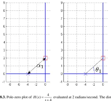
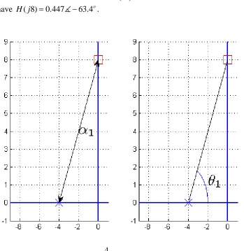
use the pole zero plot to determine the frequency response at frequencies ω0=2, 5, and 8 radians/sec. We will first look at the magnitude and then the phase of H j( ω0) for the three frequencies. Figures 8.3-8.5 shows the corresponding pole-zero plots and the distances we need to compute.
At a frequency of 2 radians/second (Figure 8.3), we first need to compute the distance between the pole at -4 and the point j2, so we have
2 2
1 ( 4 0) (0 2) 20
α = − − + − = and then
1 4
| ( 2) | 0.894
20 K
H j α
= = =
We next need to determine the angle between the pole at -4 and the point , which we can compute as
2 j
1 1
2
tan 26.6
4
o
θ = − ⎛ ⎞= ⎜ ⎟ ⎝ ⎠
[image:9.612.127.483.324.651.2]Hence the phase is−26.6o. Thus we have H j( 2)=0.894(−26.6.o.
Figure 8.3. Pole-zero plot of
4 4 ( ) H s
s =
+ evaluated at 2 radians/second. The distance between the pole and the point is used in the magnitude computation, while the angle between the pole and the point is used in the phase computation.
2 j
2 j
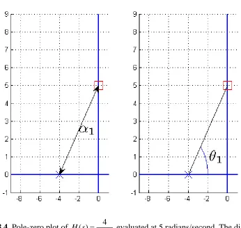
At a frequency of 5 radians/second (Figure 8.4), we need to compute the distance between the pole at -4 and the point j5 so we have
2 2
1 ( 4 0) (0 5) 41
α = − − + − = and then
1 4
| ( 5) | 0. 25
1 6
4 K H j
α
= = =
Similarly, to compute the phase we need the angle between the pole at -4 and the point , so we have
5 j
1 1
5
tan 51.3
4
o
[image:10.612.131.477.271.598.2]θ = − ⎛ ⎞= ⎜ ⎟ ⎝ ⎠ and henceH j( 5)=0.25(−51.3o.
Figure 8.4. Pole-zero plot of
4 4 ( ) H s
s =
+ evaluated at 5 radians/second. The distance between the pole and the point is used in the magnitude computation, while the angle between the pole and the point is used in the phase computation.
5 j
5 j
At a frequency of 8 radians/second (Figure 8.5), we need to compute the distance between the pole at -4 and the point j8, so we have
2 2
1 ( 4 0) (0 8) 80
α = − − + − =
and then
1 4
| ( 8) | 0. 47
0 4
8 K H j
α
= = =
The phase is given by
1 1
8
63.4 4
tan o
θ − ⎛ ⎞ = ⎜ ⎟ ⎝ ⎠ =
[image:11.612.132.481.178.537.2]and we have H j( 8)=0.447(−63.4o.
Figure 8.5. Pole-zero plot of
4 4 ( ) H s
s =
+ evaluated at 8 radians/second. The distance between the pole and the point is used in the magnitude computation, while the angle between the pole and the point is used in the phase computation.
8 j
8 j
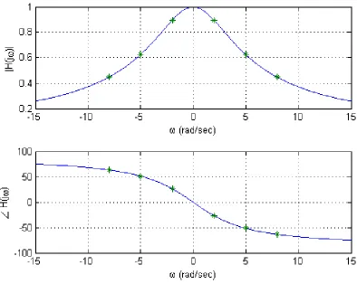
Figure 8.6 displays the magnitude and phase as a continuous function of frequency, with the points we just calculated shown with a star. Note that the magnitude is an even function of the frequency, and the phase is an odd function of the frequency.
Figure 8.6. Magnitude and phase plots of
4 4 ( ) H s
s =
+ . The stars (*) are located the at discrete points we evaluated in Example 8.3.1.
Example 8.3.2. Consider the system with transfer function 2
2
20 200 ( 10 10 )( 10 10 )
( 16 80)( 10) ( 8 4 )( 8 4 )(
)
10)
( s s s j s
H j
s s s s j s j s
s + + = + + + −
+ + + + + + − +
=
Use the pole-zero diagram to determineH j( 2). The appropriate pole-zero diagram is shown in Figure 8.7. Computing the distances and angles between the zeros and the point
we have 2
j
2 2 1
1 1
2 2 1
2 2
8
( 10 0) (10 2) 12.806, tan 38.66
10 12
( 10 0) ( 10 2) 244 15.621, tan
164
50.19 10
o
o
β φ
β φ
−
− − ⎛ ⎞
= − − + − = = = ⎜ ⎟= −
⎝ ⎠ ⎛ ⎞
= − − + − − = = = ⎜ ⎟=
⎝ ⎠
Computing the distances and angles between the poles and the point j2 we have
2 2 1
1 1
2 2 1
2 2
2 2 1
3 3
2
( 10 0) (0 2) 104 10.198, tan 11.31
10 2
( 8 0) (4 2) 68 8.246, tan 14.04
8 6
( 8 0) ( 4 2) 100 10.000, tan 36.87
8
o
o
o
α θ
α θ
α θ
−
−
− ⎛ ⎞
= − − + − = = = ⎜ ⎟=
⎝ ⎠ − ⎛ ⎞
= − − + − = = = ⎜ ⎟= −
⎝ ⎠ ⎛ ⎞
= − − + − − = = = ⎜ ⎟=
⎝ ⎠
We can then compute 1 2 1 2 3
1 2 1 2 3
(12.806)(15.621)
0.238 (10.198)(8.246)(10)
( | ( 2) |
38.66
2) o 50.19o 11.31o 14.04o 36.87o 22.6
H H j
j o
β β α α α
φ φ θ θ θ
= ≈
= + − − − =
=− + − + −
( ≈ −
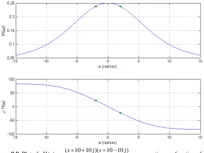
A plot of the magnitude and phase of this transfer function as a continuous function of frequency is shown in Figure 8.8. In this figure, the point on the plot we just computed is identified with a star (*).
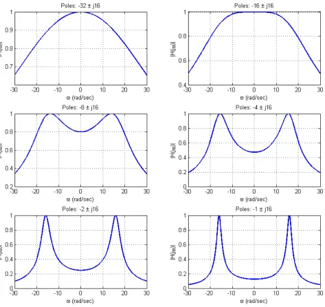
While computing the magnitude and phase of the transfer function this way can become quite tedious if we need to compute it for many frequencies, it does help to visualize the frequency response. For example, if a system has a single real pole at−p, then the smallest the distance between this point and any point on the jω axis occurs whenω=0. This means the maximum of |H j( ω) |occurs when ω=0 and will be monotonically decreasing in magnitude as the frequency increase. If a system has two complex conjugate poles, such as at − ±σ jω0, then at the frequency ω ω= 0 the denominator tends to have its smallest value, and the magnitude of the transfer function its largest value. This is not always true, but is a general trend especially when the imaginary part of the pole is large compared to the real part of the pole (ω0 >>σ ). Figure 8-9 demonstrates this type of behavior. In this figure, the imaginary part of the pole is fixed at as the real part varies. The magnitude of each plot is scaled to a maximum of one. As the figure shows, as the magnitude of the imaginary part of the pole becomes larger than the
magnitude of the real part of the pole, we see peaks or resonances at the frequency corresponding to the imaginary part of the poles.
16 ±
Figure 8.7. Pole-zero diagram for Example 8.3.2. We are evaluating the transfer
function ( 10 10 )( 10 10 )
( 8 4 )( 8 4 )( 10)
( ) s j s
j s
s
s s j
H + + + −
+ + − +
= +
j
at the frequency 2 radians/sec.
Figure 8.8. Plot of ( 10 10 )( 10 10 ) ( 8 4 )( 8 4 )( 10)
( ) s j s
j s
s
s s j
H + + + −
+ + − +
= +
j
as a continuous function of frequency. This is the transfer function from Example 8.3.2, and the stars (*) denote the points we computed in that example.
Figure 8.9. This figure shows the magnitude of the frequency response of various systems that have two complex conjugate poles. All of these systems have poles of the form σ ±16 where the real part of the pole varies from -32 to -1. The magnitudes for these systems have been scaled to have a maximum value of one.
8.4 Using Decibels
Before the advent of calculators and computers, people needed an easy way to sketch frequency response plots, and it was determined that the use of a logarithmic scale was the best choice. This is primarily because of the following relationships
log( ) log( ) log( ) log( / ) log( )
) log( )
log( ) log( N
ab a b
a b b
a N a
a
= +
= =
−
In many engineering systems, we are interested in the relationship between the input and the output. One very useful measure for many applications is to measure the ratio of the output power to the input power, so this idea is also included in our measurement scale. We then define the power gain G in decibels (or dBs) as
10 10 log out dB
in P G
P
⎛ ⎞
= ⎜ ⎟
⎝ ⎠
Note that we are using a base ten logarithmic scale. If we think about a circuit, we often want to measure the ratio of the output voltage (or current) to the input voltage (or
current). It is customary to assume we measure the voltage across (or through) a common resistance (typically we assume 1 ohm), so we have
2 2
10 2 10 2 10
| / | |
10 log | 10 |
| log | 20 log
| / | | |
out out out
dB
in in in
V R V V
G
V R V V
⎡ ⎤ ⎡ ⎤ ⎡
= ⎢ ⎥= ⎢ ⎥= ⎢
⎣ ⎦ ⎣ ⎦ ⎣
|⎤ ⎥ ⎦
Now note that if we have a transfer function relating the input and output, ( ) ( ) ( )
out s H s Vin
V = s
then we have
| ( ) |
| ( ) | ( ) |
out
in
V s
H s
V s = |
and
10 10
| |
20 log 20 log | |
| |
out dB
in V
G H
V
⎡ ⎤
= ⎢ ⎥=
⎣ ⎦
We can also measure the power with respect to a known reference power. The reference power is measured as the rms value of the signal across (through) a 1 ohm resistor. However, since we are assuming the common one ohm resistor, we just reference it to an rms voltage. For example, to measure a signal in dBV, we reference the signal to a 1 volt rms signal,
10 20 log
1 ( )
rms dBV
V G
volt rms
⎡ ⎤
= ⎢ ⎥
⎣ ⎦
To measure power in dBmV, we reference our signal to a 1 mV rms signal, and compute it as
10 20 log
1 (
rms dBmV
V G
millivolt rms)
⎡ ⎤
= ⎢ ⎥
⎣ ⎦
In what follows, we will just use the convention above, that 10
20 log | ( ) |
dB
G = H jω
8.5 Bode Plots
A very common method of representing the frequency response of a transfer function is with a Bode plot. This form of representation was very important before the advent of computers. However, it is still very useful to be able to quickly sketch Bode plots to estimate the frequency response of a system, and also to be able to determine how the frequency response may change as poles and zeros are added to a transfer function. The Bode plot is based on knowledge of how to construct the Bode plot for basic building blocks that make up our transfer functions and then combining the Bode plots for these basic building blocks into the Bode plot for the entire transfer function. The ability to easily combine the Bode plots of the building blocks is based on the properties of the polar form of writing complex functions of frequency and properties of the logarithm,. The building blocks that make up the transfer functions we have been studying are the following:
• Constant gains, K
• Integrators or differentiators, sn • Simple poles or zeros,
(
τs+1)
n• Complex conjugate poles or zeros, 12 2 2 1
n
n n
s ζ s
ω ω
⎛ ⎞
+ +
⎜ ⎟
⎝ ⎠
Basically, any transfer function we have studied (except for those with delays) can be written as a combination of these building blocks.
Next, let’s assume we have two complex functions, A j( ω)and B j( ω). We can represent these in polar form as
A(j (j ) ) ) | ( ) |
( |
( )
(
) | B
j
j A j
B
A j e
B
j j e
ω
ω
ω ω
ω ω
= =
(
(
Let’s now look at two new functions of these basic functions,
1 2 ( ) ( ) ( ) ( ) ( ) ( ) j A j B j
A j Z j
B j
Z ω ω ω
ω ω
ω =
=
If we write these new functions in polar form we will have
( ) ( ) ( ( ) ( ))
1
( )
( ( ) ( ))
2 ( )
( ) | ( ) | | ( ) | | ( ) || ( ) |
| ( ) | | ( ) |
( )
| ( ) | | ( ) |
j A j j B j j A j B j
j A j
j A j B j j B j
Z j A j e B j e A j B j e
A j e A j
Z j e
B j e B j
ω ω ω
ω
ω ω
ω
ω ω ω ω ω
ω ω ω ω ω + − = = = = ( ( ( ( ( ( ( ω (
Then we can write the magnitudes and phases as,
1 1 2 2 | ( ) | | ( ) || ( ) | ( ) ( ) ( ) | ( ) | | ( ) | ( ) ( ) ( ) | ( ) |
Z j A j B j Z j A j B j
A j
Z j Z j A j
B j B j
ω ω ω ω ω
ω
ω
ω ω ω
ω
= =
= =
( ( (
( ( ( ω
+ −
Represent the magnitudes in terms of dBs, then we have
[
]
1 10 10 10
2 10 10 10
| ( ) | 20 log | ( ) || ( ) | 20 log | ( ) | 20 log | ( ) | | ( ) | ) | | ( ) |
| ( ) | 20 log 20 log | ( ) | 20 log | ( ) | | ( ) | | ( ) | | (
(
) |
|
dB db dB
dB dB dB
Z j A j B j A j B j A j
A j
Z j A j B j A j B j
B j
B j
ω ω ω ω ω ω
ω
ω ω ω ω
ω = = + = ⎡ ⎤ = ⎢ ⎥= − = − ⎣ ⎦ + ω ω
Finally, representing the magnitude in dB and the phase in either degrees or radians we have 1 1 2 1 | ( ) | | ( ) | ) | ( ) ( ) ( ) | ( ) | | ( ) | | ( ) | | ( ) ( ( ) ( )
dB db dB
dB dB dB
Z j A j Z j A j B j
Z j A j B j Z j A j
j
B B
j
ω ω ω ω ω ω
ω ω ω ω ω
= =
= −
+
= +
( ( (
( ( ( ω
+
It is these simple relationships that form the basis of constructing the Bode plot. We basically need to figure out how to plot the magnitude or phase of a building block function, and then add the responses. Note that a Bode plot really refers to two different plots, a magnitude plot and a phase plot. Finally, it will be convenient to plot the Bode plots as semi-log plots, where the frequency axis is plotted on a logarithmic scale and the magnitude (in dB) or phase is plotted on a linear scale.
8.5.1. Constant Terms
The first building block is the constant term in the transfer function, H j( ω)=K
o
. We can represent this in terms of magnitude and phase as . It is important to note that the magnitude must be zero or positive. Hence if the gain is negative, then this will be included in the phase. For example, we can write . Next, when we look at the magnitude we have
) | |
( K j K
H jω = e(
180 8 8ej
− =
10 |H j( ω) |dB=20 log |K| We can break this into three regions
10 10 10 0 | | 1 20 log
| | 1 20 l
| | 0 | | og | | 1 20 lo
0 | | 0 g
K K K
K K K
< < = >
< = >
In summary, the magnitude plot of a constant will be a flat line, and the phase plot will also be a flat line.
8.5.2. Integrators and Differentiators
The transfer function for these building blocks are of the formH s( )=snwherencan be positive (differentiators) or negative (integrators). To determine the frequency response we look at
(
90)
90 ) ( )( o o
n
n j n jn
j
H jω = ω = ωe =ω e
The phase of this building block is then easy to determine as , which is just a constant. To determine the magnitude part, we have
90o n
10 10
20 log ωn =n20 log ω
At this point, it is important to note that when ω=1 we have 20 log10ω=20log101=0, so the point (1,0) will be on the Bode plot for this building block. Next, let’s see how much the magnitude changes as the frequency changes by a factor of 10 (a decade). To do this, let’s assume that at some frequencyω1 we have , and then we have another frequency
1 10
a
ω = 2
ω a decade later, 1 2 10
a
ω = +
. Looking at the magnitudes for these frequencies we have
10 1 10 1 10
1
10 2 10 2 10
20 log 20 log 20
20 lo
20 log 10
20 lo
g g 20 log 10 20
n a
n a
n n n a
n n
n
ω ω
ω ω + =
= =
(a 1)
= +
=
=
Thus in a decade (factor of 10) change in frequency, the magnitude changes by 20 dB. This is corresponds to a slope of 20n dB/decade.
n
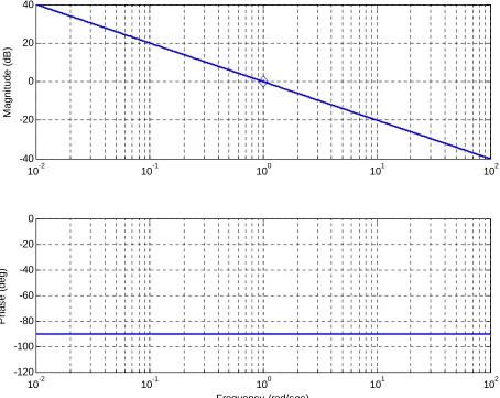
Example 8.5.1. Sketch the Bode plot for the transfer functionG s( ) 1 s
= . The magnitude of this transfer function goes through the point and has a slope of -20 dB/decade. The phase is a constant . The Bode plot for this system is shown in Figure 8.10.
(0 dB,1 rad / sec) 90o
−
Example 8.5.2. Sketch the Bode plot for the transfer function G s( )=s2. The magnitude of this transfer function goes through the point and has a slope of +40 dB/decade. The phase is a constant . The Bode plot for this system is shown in Figure 8.11.
(0 dB,1 rad / sec) 180o
−
Example 8.5.3. Sketch the Bode plot for the transfer function ( ) 100 s
G s = . Note that there are two building blocks for this example,G s( ) 100 1 G s1( ) G s2( )
s
= × = × . We will
construct the Bode plot for the individual components, and then add them. For we have
1( ) 100
G s = 20 log 10010 =40dB and the phase is 0o. For G s2( ) 1 s = the magnitude goes through the point ( with a slope of – 20 dB/decade, and the phase is a constant . The Bode plots for and are shown in Figure 8.12 as dashed lines. The Bode plot for is then determined by adding these components, and is displayed as a solid line in Figure 8.12.
0 dB,1 90o
−
( ) G s
rad / sec) 1
G G2
10-2 10-1 100 101 102
-40 -20 0 20 40
M
a
gni
tud
e (
dB
)
10-2 10-1 100 101 102
-120 -100 -80 -60 -40 -20 0
P
h
as
e (
de
g)
[image:21.612.97.551.257.618.2]Frequency (rad/sec)
Figure 8.10. Bode plot of the transfer function G s( )=s2. Note that that a diamond delineates the point (0 dB,1 rad / sec).
Figure 8.11. Bode plot of the transfer function G s( ) 1 s
= . Note that that a diamond delineates the point (0 dB,1 rad / sec).
10-1 100 101 102
-40 -20 0 20 40 60 80
M
a
g
ni
tud
e (
d
B
)
10-1 100 101 102
-210 -200 -190 -180 -170 -160 -150
P
h
as
e
(
d
eg
)
Frequency (rad/sec)
Figure 8.12. Bode plot of the transfer function ( ) 100 s
G s = . The Bode plots of the two subcomponents are shown as dashed lines, the final Bode plot is shown as a solid line. In the phase diagram, the subcomponent at -90 degrees overlaps with the final phase of -90 degrees (since the other subcomponent’s phase is zero). Note that the sum of any two values (at a given frequency) on the dashed lines equals the value on the solid line at the same frequency.
10-1 100 101 102
-40 -20 0 20 40 60
M
ag
ni
tude
(
d
B
)
10-1 100 101 102
-100 -50 0
Ph
as
e
(d
eg
)
Frequency (rad/sec)
8.5.3. Simple Poles and Zeros
This building block has the form H(s)=(τs+1)n where again n is negative (for a pole) and positive (for a zero). To get the frequency response, we look at
1 1
tan tan
2 1 2 2 1
) ( 1) ) 1 ( ) 1
( (
n
n
j j
n
j j e
H e
n
τω τ
ω = τ ω+ ⎢⎡ τω + −⎝⎜⎛ ⎠⎞⎟⎤⎥ ⎡τω + ⎤ −⎝⎛⎜ ⎠⎞⎟
⎣ ⎦
⎢ ⎥
⎣ ⎦ =
=
ω
The phase response is
1 ) tan
1
( n
H jω = − ⎛⎜ωτ ⎞⎟ ⎝ ⎠ (
Rather than trying to exactly determine what this looks like, let’s just look at a few points. For small frequencies,ω≈0, we have ) tan 1 0
1
( n
H jω ≈ − ⎛ ⎞⎜ ⎟≈0 ⎝ ⎠
( . For very large
frequencies, ω≈ ∞, we have ) tan 1 90 1
( H j
( o
n n
ω ≈ − ⎛ ⎞∞ ≈ ⎜ ⎟
⎝ ⎠ . Finally, when 1 ω
τ = we
have ω) tan 1 1 1 (
H j ≈ − ⎛ ⎞⎜ ⎟≈ ⎝ ⎠
( n n45o.
A more precise formula is as follows:
0.1 1
( ) 0
1
( ) 45
10 1
( ) 90
o
o
o
H j one decade before
H j n
H j n one decade after
ω ω τ τ ω ω τ ω ω τ τ ⎛ ⎞ ≈ = ⎜ ⎟ ⎝ ⎠ ≈ = ⎛ ⎞ ≈ = ⎜ ⎟ ⎝ ⎠ ( ( (
When we sketch the phase as follows: for ω 0.1 τ
< the phase is zero, and for ω 10 τ > the phase isn90o. We then connect these points with a straight line.
The magnitude response is | ( ) | ( )2 1 2
n
H jω =⎡⎣τω + ⎤⎦ , and again we will look at three points. For small frequencies, ω≈0, we have |H j( ω) |dB≈20log10(1)≈0. For large very
frequencies, ω≈ ∞, we have
2 2
10 10 10 10 10
) | 20 log ) 20 log ) 20 log 20 log 20
| ( ( (
n
dB
H jω ≈ ⎣⎡τω ⎤⎦ =n τω =n τ +n ω≈n l go ω
This means that for large frequencies we will have a slope of 20n dB/decade. Finally, when ω 1
τ
= we have
[ ]
210 10
) | 20 log 2 10 log
| ( (2) 3
n
dB
H jω = =n = n. Summarizing these
results we have
0.1 1
0 0 ( ) 0
1
3 ( ) 45
10 1
20 / ( ) 90
o
o
o
Magnitude Phase
dB H j one decade before
n dB H j n
slope n dB decade H j n at one decade aft
at
er
ω ω ω
τ τ
ω ω
τ
ω ω ω
τ τ
⎛ ⎞
≈ ≈ = ⎜ ⎟
⎝ ⎠
= ≈
⎛ ⎞
≈ ∞ ≈ ≈ = ⎜ ⎟
⎝ ⎠
(
( (
Example 8.5.5. Sketch the Bode plot for the transfer function 1 0.1 1 ( )
G s
s+
= . Here we
have 1 10
τ = , and this is referred to as the break or corner frequency. The magnitude is then zero until ω 10 1
τ
= = . At this point the magnitude decreases linearly with a slope of -20 dB/decade. Both the approximate (straight line) approximation and true magnitude portion of the Bode plot is shown in the top panel of Figure 8.13. The approximate magnitude is shown in the dashed line while the true magnitude is shown as a solid line. Note that at the corner frequency there is a difference of approximately 3 dB between the estimate and true magnitude plot. The phase plot is zero until 0.1 0.1 10 1
τ = × = and is for frequencies above
90o
− 10= 10 10 100
τ × = . Between these points we draw a straight line. The estimated phase plot (dashed line) and true phase plots are shown in the lower panel of Figure 8.13.
Example 8.5.6 Sketch the Bode plot for the transfer function
2
1 1
1 100 10 ( )
0 G s = ⎛⎜ s+ ⎞⎟
⎝ ⎠ .
This transfer function is again made up of two building blocks, 1( ) 1 100
G s = and
2 2
1
( ) 1
100 G s =⎛⎜ s+
⎝ ⎠
⎞
⎟ . The magnitude of the first building block is just the constant dB and the phase is zero. The corner frequency for the second building block is 100 rad/sec. The magnitude of the estimate will be zero before this corner point, and will have a positive slope of 40 dB/decade for frequencies above this. The phase of this component will be zero until 10 rad/sec, and will be 180 for
frequencies above 1000 rad/sec. The estimated phase will be linear between these points. The estimated magnitude and phase plots, as well as the correct magnitude and phase plots, are shown in Figure 8.14. In this plot, the building block estimates are dashed lines, the sum of the building blocks are dotted lines, and the correct plots are shown as solid lines.
10 0.01 20 log ( )= −40
o
Example 8.5.7. Sketch the Bode plot approximation for the transfer function 100 ( ( ) 10) s s G s +
= . First we need to put this into the correct form,
100 100 10
( 10) 10 (0.1 1) (0.1
)
) (
1
s s s s s
G s s = = + × × + = + We will then have three components, or building blocks,
1 2 1 3 ( ) 1 ( ) 1
( ) 1
1 1 0 0 s s s
G s s
G G − = ⎛ ⎞ =⎜ + ⎟ ⎝ ⎠ =
The straight line approximations for the building blocks, and the final Bode plot are shown in Figure 8.15.
Example 8.5.8. Sketch the Bode plot for the transfer function ( ) 1 ( 10)( 100)
s G s s s + = + + .
Again, we first need to put this into the correct form,
3
1 1 10
( )
( 10)( 100) 10 (0.1 1) 100 (0.01 1) (0.1 1)(0.01 1)
s s
G s
s s s s s s
−
+ +
= = =
+ + × + × × + + +
(s+1) The building blocks are then
3 1 2 1 3 1 4
( ) 10 ( ) ( 1) ( ) (0.1 1) ( ) (0.01 1) G s
s s
G s s
s G s G − − − = = + = + = +
The straight line approximation for the building blocks, and the final Bode plot are shown in Figure 8.16.
Example 8.5.9. Sketch the Bode plot for the transfer function ( ) 10 2 ( 100)
s G s
s
=
+ . Putting this transfer function into the correct form and identifying the building blocks we have
(
)
3 2
2 2
10 10 10
( )
( 100) 100 (0.01 1) (0.01 1)
s
s s
G s
s s s
− = = = + × + + 3 1 2 2 3
( ) 10 ( )
( ) (0.01 1) G G G s s s s s − − = = = +
The straight line approximation for the building blocks, and the final Bode plot are shown in Figure 8.17.
Figure 8.13. Bode plot for the transfer function 1 0.1 1 ( )
G s
s+
= . Note the 3 dB
discrepancy at the corner frequency in the magnitude plot. The Bode plot of the straight line approximation is shown as dashed lines while the exact Bode plot is shown as a solid line.
10-1 100 101 102 103
-50 -40 -30 -20 -10 0 10
M
agni
tude (dB
)
Frequency (rad/sec)
10-1 100 101 102 103
-100 -80 -60 -40 -20 0
P
has
e (deg)
Frequency (rad/sec)
100 101 102 103 104 -40
-20 0 20 40
M
agni
tud
e (
d
B
)
Frequency (rad/sec)
100 101 102 103 104
0 50 100 150 200
P
h
as
e (
deg)
[image:28.612.99.543.85.468.2]Frequency (rad/sec)
Figure 8.14. Bode plot for the transfer function
2
1 1
1 100 10 ( )
0 G s = ⎛⎜ s+ ⎞
⎝ ⎠⎟ . Note the 6 dB discrepancy at the corner frequency in the magnitude plot. The straight line
approximations of the individual components are shown as dashed lines, the actual Bode plot is shown as a continuous line. Note that for any given frequency, if you sum the values of the straight line approximations you get reasonable approximations to the true (continuous curve) Bode plot.
10-1 100 101 102 103 -80
-60 -40 -20 0 20 40
M
agni
tude (dB
)
Frequency (rad/sec)
10-1 100 101 102 103
-200 -150 -100 -50 0 50
P
has
e (d
eg)
[image:29.612.94.567.85.495.2]Frequency (rad/sec)
Figure 8.15. Bode plot for the transfer function 100 10 ( 10
(
) (
)
0.1 1
s s s s
G s = =
)
+ + . The
straight line approximations of the individual components are shown as dashed lines, the actual Bode plot is shown as a continuous line. Note that for any given frequency, if you sum the values of the straight line approximations you get reasonable approximations to the true (continuous curve) Bode plot.
10-1 100 101 102 103 104 -80
-60 -40 -20 0 20 40 60 80
M
ag
ni
tude
(
d
B
)
Frequency (rad/sec)
10-1 100 101 102 103 104
-100 -50 0 50 100
P
h
as
e
(
d
eg
)
[image:30.612.97.569.88.501.2]Frequency (rad/sec)
Figure 8.16. Bode plot for the transfer function
3 10 ( 1) ( )
(0.1 1)(0.01 1)
s G s
s s
− +
=
+ + . The straight line approximations of the individual components are shown as dashed lines, the actual Bode plot is shown as a continuous line. Note that for any given frequency, if you sum the values of the straight line approximations you get reasonable approximations to the true (continuous curve) Bode plot.
Figure 8.17. Bode plot for the transfer function.
3 2 10 ( )
(0.01 1)
s G s
s
− =
+ The straight line approximations of the individual components are shown as dashed lines, the actual Bode plot is shown as a continuous line. Note that for any given frequency, if you sum the values of the straight line approximations you get reasonable approximations to the true (continuous curve) Bode plot.
100 101 102 103 104
-100 -50 0 50 100
M
agni
tude (
dB
)
Frequency (rad/sec)
100 101 102 103 104
-200 -150 -100 -50 0 50 100
P
has
e (
deg)
Frequency (rad/sec)
8.5.3. Complex Conjugate Poles and Zeros
The basic building block for a system with complex conjugate poles or zeros can be put into the standard form
2 2
1 2
( ) 1
n
n n
G s s ζ s
ω ω
⎛ ⎞
=⎜ + + ⎟
⎝ ⎠
Evaluating this at s= jωwe get
(
)
22
( ) 1 2 1 j2
n
n
n n
j u
G jω ω ζ ω
ω ω ⎛ ⎡ ⎤ ⎞ ⎜ −⎢ ⎥ + ⎟ − + ⎜ ⎣ ⎟ = ⎝ ⎠ =
⎦ ζu
where we have defined
n
u ω ω
= . Computing the magnitude and phase we have
2 2 2 1
2
, 2
| ( ) | (1 ) (2 ) ( ) tan
1
n u
G j u u G j n
u ζ
ω =⎡ − + ζ ⎤ ∠ ω = − ⎛ ⎞
⎦ ⎜ − ⎟
⎣ ⎝ ⎠
Let’s first look at the magnitude in decibels,
2 2 2 2 2 2 2
10 10
) | [(1 ) (2 )
| ( 20 log ] 10 log [(1 ) (2 ]
n
dB
G jω = −u + ζu = n −u + ζu)
For ω≈0we have u≈0, and|G j( ω) | 1≈ , so |G jω( ) |dB≈0. For larger frequencies, ω >>ωn, we have
4 4 ( | | ) n n n
G jω u ω ω ⎛ ⎞ ≈ = ⎜ ⎟
⎝ ⎠ , so in decibels we have 4
10 10 10 10 10
|G j( ω) |dB≈10nlog [u ]=40 logn u=40 logn ω−40nlog ωn ≈40nlog ω So for large frequencies we have a slope of 40n dB/decade.
For ω ω≈ nwe have u≈1. Then we have|G jω( ) | (2 )≈ ζ n, and in decibels,
( )
10
) | 20 2
|G(jω dB≈ nlog ζ
Now if we have two regions to consider,
10 10
0 log
0
0.5 (2 )
1 (2 )
.5 log 0 0 ζ ζ ζ ζ < < < < > <
Figure 8.18 displays the magnitude plot of a the second order system 2
2 2
2
( ) n
n n
G s K
s s
ω
ζω ω
+ +
=
forK =10,ωn =2 ,0 and ζ =0.01, 0.1, 0.250.5, 0.75, 0.99. Note that there is a sharp peak at the resonant frequency, which is given by ωr =ωn 1 2− ζ2 . Not that for
0.5 0.707
ζ > = there is no resonance. As this figure shows, the smaller the damping ratio, the higher the peak frequency will be.
Now we need to look at the phase of the response of this system. For low frequencies,
we have . For large frequencies,
0
u≈ 1
( ) tan (2 ) 0o
G jω n − ζu
∠ ≈ = ω>>ωn we have
1 2 (
G jω) ntan− ζ n180o
∠ ≈ ≈
−∞ . Finally, forω ω= n (u=1) we have
1 2
( ) tan 90
0
o
G jω n − ⎛ ζ ⎞ n
∠ = ⎜ ⎟=
⎝ ⎠ . Figure 8.19 shows the phase plot of the second order system
2
2 2
2
( ) n
n n
G s K
s s
ω
ζω ω
+ +
= forK =10,ωn =2 ,0 and ζ =0.01, 0.1, 0.250.5, 0.75, 0.99. Notice that as the damping ratio is smaller, the phase transition is much sharper. Also notice that all of the phase plots pass through −90owhen
20 rad/sec
n
ω ω= = .
We can then summarize our rules as
(
)
(
)
0 0 ) 0
10
( ) 45
40 / 10
n
n
o n
o
n n
Magnitude Phase
dB one decade before
depends on H j n
slope n dB decade one decade after
at
at ω ω
ω ω ζ ω
(
( ) 180
o H j
H j n
ω ω ω
ω ω ω ω
=
= ≈
≈ ∞ ≈ =
(
ω
≈ ≈
≈ (
(
8.6 Bandwidth, Filter Types, and Quality Factor
How a system affects an input signal is often used to classify the system type in terms of its filtering characteristics. Sometimes, when we are designing a control system for example, we are primarily concerned with making the output match the input with a reasonable transient response, and are not primarily concerned with the frequency
response of our system. In other situations, such as designing a circuit for a music system, we are designing a system to enhance or remove frequencies from the input signal. In these cases we are interested in talking about these filtering characteristics that are most relevant in those applications. Three of the most useful system characteristics in filtering applications are the bandwidth of the filter, the filter type, and the quality of the filter.
100 101 102 103 -60
-40 -20 0 20 40 60
M
agni
tude
(
d
B
)
Frequency (rad/sec)
0.01
0.5
[image:34.612.93.568.96.464.2]0.99
Figure 8.18. Magnitude of the frequency response for the transfer function 2
2 2
2
( ) n
n n
G s K
s s
ω
ζω ω
+ +
= forK =10,ωn =2 ,0 and ζ =0.01, 0.1, 0.250.5, 0.75, 0.99
10-1 100 101 102 103 -200
-150 -100 -50 0 50
P
h
ase (
d
eg
)
Frequency (rad/sec)
0.01
0.5
0.99
Figure 8.19. Magnitude of the frequency response for the transfer function 2
2 2
2
( ) n
n n
G s K
s s
ω
ζω ω
+ +
= forK =10,ωn =2 ,0 and ζ =0.01, 0.1, 0.250.5, 0.75, 0.99
8.6.1 System Bandwidth
The system bandwidth is usually defined as the frequency range for which the power of the output is within one half of the peak output power. Thus we determine the bandwidth as the difference between the minimum and maximum frequencies as which
1 ( )
2
max
out Pout
P ω = In terms of dB’s we have
[
]
10 10 10 10
1 1
( ) 10log 10 log 10 log
2 2
10 log Pout ω Poutmax outmax
⎡ ⎤ ⎡ ⎤ ⎡ ⎤
= ⎢ ⎥= ⎢ ⎥+ ⎣ ⎦
⎣ ⎦ ⎣ ⎦ P
Then we have
10 1
10 log 3 dB
2 ⎡ ⎤ ≈ − ⎢ ⎥ ⎣ ⎦ Hence we determine the bandwidth as
high low
Bandwidth=ω −ω where
10 10
10 log [ ( )] 10 log [ ] 3 dB
low max
max
out out
P P
ω ≤ ≤ω ω ω ≥ −
This form is useful for reading information off of Bode plots. Sometimes we don’t want to have to convert to Bode plots. Then we can just use
1 ( )
2
low max
max
out Pout
P
ω ≤ ≤ω ωω ≥ In terms of transfer functions, we have
1
| ( ) | | ( ) |
2
low max
max
H j H j
ω ≤ ≤ω ωω ≥ ω
or
[
]
10 | ( ) | 10 ) |
10 log 10 log | ( 3 dB
low max
max
H j
H j
ω ω ω
ω ω
≤ ≤
≥ −
Example 8.6.1. Consider the RC circuit shown in Figure ??, The transfer function for this circuit is clearly
1 ( ) 1 H s RCs = + In terms of frequency response we have
1 ( ) 1 H j j RC ω ω = + The magnitude of the transfer function is then
2 1 ) | ( ( ) 1 | RC H jω
ω =
+
Clearly the maximum of this transfer function occurs when ω=0, so for this system |Hmax(jω) |=1
We next need to find the frequency at which
| ( ) | 1 | ( ) |= 1
2 2
max H
j j
H ω ≤ ω
Since our transfer function is a decreasing function of frequency, we can just find the largest frequency for which this is true,
2
1 | ( ) |
2 )
1
( 1
H j
RC ω
ω + = =
which leads to RCω=1, or 1 RC
ω= . Thus the bandwidth for this system is
1 1
0
high low
RC R
ω −ω = − = C
f
A Bode plot of the magnitude of this transfer function for R=1kΩ,C=1μ is shown in Figure 8.21. We expect the bandwidth to be 1 1000
[image:37.612.213.400.288.409.2]RC = rad/sec. The maximum value of the transfer function is 1 (or 0 dB), and the bandwidth is then the frequency at which the magnitude has dropped 3 dB. This Bode plot has a dashed line at the -3 dB point, and you can see it intersects the magnitude of the transfer function at 1000 rad/sec.
Figure 8.20. RC circuit for Example 8.6.1.
Figure 8.22 displays three different bandpass systems with bandwidths of 400, 100, and 50 radians/sec. In these figures, the -3 dB line is shown as a dashed line, and is measured from the peak amplitude.
100 101 102 103 104 -25
-20 -15 -10 -5 0
M
agni
tud
e (
dB
)
[image:38.612.101.554.87.453.2]Frequency (rad/sec)
Figure 8.21. Bode plot of the magnitude of the transfer function for Example 8.6.1. The maximum value of the transfer function is 1 (0 dB), so the bandwidth will be determined by the point where the magnitude falls to – 3dB. This occurs at 1000 rad/sec.
101 102 103 40
45 50 55 60 65
M
agni
tude
(
d
B
)
Frequency (rad/sec)
101 102 103
25 30 35 40 45
M
a
gni
tude
(
d
B
)
Frequency (rad/sec)
101 102 103
-20 -15 -10 -5 0 5
M
a
gn
it
ud
e
(
d
B
)
[image:39.612.91.585.85.500.2]Frequency (rad/sec)
Figure 8.22. Three different bandpass systems with bandwidths of 400, 100, and 50 radians/sec. The -3 dB line is shown as a dashed line, and is measured from the peak amplitude.
8.6.2. Filter Types
In discussing filter types, it is good to remember the basic relationship that if the input signal to a stable system is ( )x t = Acos(ωot+φ)
0
( ) |cos( o
y t A H j t
, then the steady state output of the system will be ss( )= | ω ω + + ∠φ H(jωo)). The filter type is determined by the magnitude of the transfer function at various frequencies, since this directly affects the output signal. Specifically, if the magnitude of the transfer function as a specific frequency is zero, the output signal is zero. Altyernatively, if the magnitude of the
transfer function at a specific frequency is one, then the input signal passes without change. In talking about ideal filter types, this is generally what we are looking at: does the signal in a range of input frequencies pass or is the signal removed from the output. The four major filter types are displayed in Figure 8.23, as ideal filters. Note that the magnitude of the transfer function is symmetric about the real axis, and we are plotting the magnitude response for both positive and negative frequencies. Although the phase of the filter is important in some applications, it is not important in classifying the filter type.
The first characterization is the lowpass filter, and this filter passes signals with low frequencies and removes high frequencies from the input signal. Note that the lowpass filter is centered at zero frequency, but the bandwidth is only measured from 0 to the edge of the passpband. Next, a highpass filter removes all low frequencies and only allows high frequencies to pass. The bandwidth of a high pass filter is not really
[image:40.612.93.523.334.650.2]meaningful. A bandpass filter allows frequencies only in a range of frequencies to pass. Finally, a bandreject or notch filter removes only very specific frequencies. Notch filters are often used to remove 60 Hz noise from AC power systems.
Figure 8.23. Ideal lowpass, highpass, bandpass, and bandreject filters.