1
ECE-320 Lab 4: Utilizing a dsPIC30F6015 to control the speed of a wheel
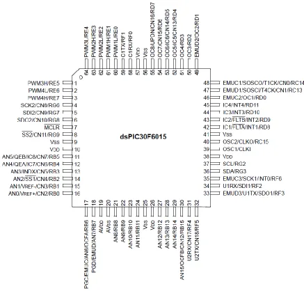
[image:1.612.81.518.195.613.2]Overview: In this lab we will utilize the dsPIC30F6015 to implement P, I, PI, PD, and PID controllers to control the speed of a wheel. You will need to start with the code you developed for the last lab. The dsPIC30F6015 has been mounted on a carrier board that allows us to communicate with a terminal (your laptop) via a USB cable. In what follows you will need to make reference to the pin out of the dsPIC30F6015 (shown in Figure 1) and the corresponding pins on the carrier (shown in Figure 2)
2
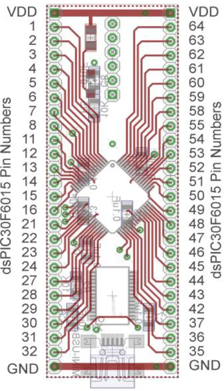
Figure 2. dsPIC30F6015 carrier. Note that the pin numbers are not consecutive.
Refer to the previous lab for connecting the input from the pot and the transducers that indicate the speed of the wheel, and the external interrupt switch. Also, when you connect the power to the wheel if the speed of the wheel is negative be sure to switch the wires.
You need to download the Matlab and Simulink files from the class website before you begin the lab.
3
PART A: Setting up the parameters
In the program DT_PID_driver.m set the value of MAX_DELTA_U to 500, and set the parameters AD_scale, Relay_on, Relay_Off, and Max_Speed to the values you determined in the last lab. Then set the values of B and b to match your discrete-time model. Finally, set the delay to match your model.
PART B: Proportional control
We now want to start with our first control scheme, proportional control. You will need to declare the variables error and kp as a doubles (at the top of the main routine). Outside of the main while loop set
kp = 1.0, and inside the main loop, after both the speed and reference input are determined, compute the error as error = R-speed. Here R is the reference input and speed is the measured output speed of the wheel in rad/sec. The control effort is then proportional to this error, so u = kp *error. This should all be done before the statement
u = u*scale/AD_scale;
or any of the limits checks on u.
Set the input to a step of 75 rad/sec (set R = 75.0, don’t read the input from the pot.)
Recompile and download the code onto the microcontroller. Prepare to log the data measured (the Matlab code assumes this file is called Step_Response_kp, but feel free to change it.) The first time you do this the power to the wheel should be shut off just to be sure everything is ok. Once it seems to be running, turn on the power to the wheel and start the system again. Run the system until steady state (not more than 8 seconds though). In the program DT_PID_driver.m set the value of kp and run the
program. Include the graph in your memo. From this graph estimate the settling time (assume it has reached steady state) and the steady state values. It is useful to use the Data Cursor tool in the figure window, and be sure to record the value from the Measured (real) data, not the model. Remember that the settling time is within 2% of the final value, not exactly the final value.
Record these values in your memo.
Stop the system and change the value of kp to 5, and then to 10. (Be sure to recompile and download after each time, and change the value of kp in the Matlab program). Include these figures in your memo and estimate the settling time and the steady state value for both of these cases. You should notice that both the settling time and the steady state error gets smaller for this first order system as kp increases.
4
PART C: Proportional control with a prefilter
Most likely your system did not equal the reference value in steady state, or not all of them. One way to get around this is to scale the input, which is implementing a prefilter. Define two new (double)
variables, Gpf and scaled_R and modify the code so you get
scaled_R = Gpf *R; error = scaled_R – speed;
Note that we do not want to just scale R, since we want to know the (original) reference input. The value of Gpf should be assigned once outside the main while loop, and now needs to be determined. Assume the reference signal is 75 rad/sec and kp is 5. Use your results from the previous problem to determine an initial guess for Gpf. Run your system for 10 seconds, and adjust your value of Gpf so the value at 10 seconds is between 74 and 76 rad/sec. Modify the Matlab code with this value of Gpf and run it. Include this graph in your memo.
PART D: Even More Proportional control with a prefilter
Make sure kp is set to 5 for this part and the value of the prefilter is what you determined in the previous part. Now we want the reference input to be from the pot rather than a set value, so modify the code appropriately.
5
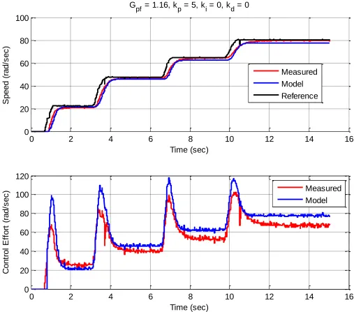
Figure 3. Proportional control with a prefilter for a staircase input.
0 2 4 6 8 10 12 14 16
0 20 40 60 80 100 G
pf = 1.16, kp = 5, ki = 0, kd = 0
Time (sec) S p e e d ( ra d /s e c ) Measured Model Reference
0 2 4 6 8 10 12 14 16
6
PART E: Integral control
Recall that using a prefilter to control steady state error can sometimes be problematic since the prefilter is outside the feedback loop. At this point, set the prefilter value to 1, but do not remove it since we will use it again. An alternative, and generally better, solution is to include some form of integral control. Recall that an integral controller has the form
1 = ) ( ) ) ( 1 ( i c
k U z
z z z G E
Rearranging this we get
1
U(z)
( )
( )
i
E z
U z
k
z
In the time-domain this becomes
( )
( )
(
1)
ie n
u n
u
k
n
Since we want the control effort as our output, we will write this as
( )
(
n
1)
i( )
n
u n
u
k e
If we assume the initial control effort is zero, we can write this as follows:
1
(1) (0) (1)
(2) (2) (1) [ (2) (1)] (3) (3) (
(1
2) [ (3) (2) e(1)]
( ) ) ( ) i i i i i i n i k
e u k e
u k
u
e u k e e
u k e u k e e
u n k e k k
Hence to implement the integral control, we need to sum the error terms and then scale them by
k
i. Declare two new (double) variables Isum and ki. Set the initial value of Isum to zero outside the main loop. Within the main loop update the error summation using something like Isum = Isum + error.Within the main loop implement a PI controller as follows:
u = kp*error + ki*Isum;
7 Your system will probably exhibit some pretty strange behavior and may not reach the correct steady state value for a while. Look at what is happening to the value of Isum during this strange behavior.
The first problem we need to fix is that our motor is only spinning in one direction. When Isum
becomes large and negative, we would expect the motor to spin in the other direction, but it can’t. One way to minimize this effect is to check to be sure that the value of Isum is greater than or equal to zero. Modify your code to do this, recompile, and run it again. (Hint: think of using the min and/or max functions.)
The second problem we have is called integrator windup. Basically, the accumulated error is becoming too large and causes the system to overshoot, and then undershoot. One way to fix this is to limit the value of Isum to a maximum value. You need to define a constant at the very beginning of the code
MAX_ISUM. You need to set a reasonable value for this variable and modify the code so the value of
Isum does not exceed this value. Modify your code to do this, recompile, download, and run it again. You will have to use some trial and error to find a good value for MAX_ISUM since it is also a function of the value of ki. Determine a value of MAX_ISUM so the percent overshoot is less than 10% and the settling time is less than 6 seconds (do not run the system more than 8 seconds, it may not have reached steady state yet but we know that in steady state it will be at 75 rad/sec). Save this run to a file (or run it again and log it this time.) Then modify DT_PID_driver.m so that it runs the Simulink file
PT_PID2.slx. This new Simulink file implements an “integrator” like our c-code. It sets and upper limit
and is really just an accumulator. You also need to set the value of MAX_ISUM, and the correct values for Gpf, kp, ki, and kd in the Matlab code. Run the Matlab code and put the resulting figure in your memo. As part of the caption estimate the percent overshoot and the estimated settling time. You will probably note that the model and the true system do not always match too well, particularly the control effort and value of Isum.
Now set the value of ki to 0.4, and modify the value of MAX_ISUM so your system has a percent overshoot less than 10% and a settling time of less than 8 seconds (don’t run your system more than 10 seconds). Log the data to a file, modify the Matlab code, and run the Matlab code to plot the measured and modeled system results. Include this graph in your memo, and indicate the percent overshoot and settling time in your caption.
The point we are trying to make here is that there is a strong dependence between the value of ISUM_MAX and ki.
PART F: Proportional plus integral (PI) control
8 The first thing we will do is to use sisotool. Start sisotool and import the plant. To construct a PI
controller, we add the P and I controllers together to get the overall transfer function:
( )
( )
1 1
p i p
i p
k k z k
k z
C z k
z z
In sisotool this will be represented as
2
( ) ( )
( )
( 1) ( 1) K z az K z a C z
z z z
In order to get the coefficients we need out of the sisotool format we equate coefficients to get:
,
p i p
k Ka k K k
When using sisotool, the maximum control effort allowed is approximately equal to
Control_Effort_Saturation/75.0
Since sisotool assumes an input of 1.0 rather than the 75.0 we are interested in. Using sisotool design a PI controller with a percent overshoot less than 20% and a settling time less than 12 seconds. (Note it may be easier to design if you remove all of the delays in the modelled plant transfer function. This is not exact, but in this case is probably close enough.) Next, implement this PI controller in your Matlab routine and run it (we don’t care what the plot of the actual system is now, we are just looking at the simulation.) Since sisotool does not assume there is a limit on the integrator (or any of the other
nonlinearities we modeled), you need to initially start with a value of MAX_ISUM of around 10000 and then reduce it to get a reasonable result. Once this is working, change your c-code to use the same parameters and run the real system. You may have to tweak the numbers a bit to get good results. Finally, run the Matlab code again and plot your simulation results with the real results. Do not run for more than 12 seconds. Include this plot in your memo. In the caption include the estimated overshoot and settling time.
An alternative method for designing a PI controller is using a trial and error method (assuming we have no model for the plant) is the following:
First, set ki = kd = 0, and try to get a good response for a step input using only kp.
Next, adjust ki to get a good steady state error. Since the integral control tends to slow the system down, don’t make this any larger than you need to. However, you may need to also change MAX_ISUM to get a good response.
For this system, limit ki to less than 1.0 and keep kp between 1.0 and 10.0.
For this part, design for a percent overshoot less than 10% and a settling time less than 5 seconds.
9 When you have good results, change the Matlab program to match the c-code, and run the Matlab
simulation plotting both results. Include this plot in your memo. In the caption include the estimated overshoot and settling time.
Finally, again modify your c-code so the input is the pot, and again run the input in a series of steps to see how well your system tracks the input (you need to let the system come to steady state before you move to the next plateau.) Include this graph in your memo. If you make the reference signal too large you will not get a steady state error of zero no matter how long you run the system. Why?
PART G: Proportional plus derivative control with a prefilter
We need to include a derivative term to implement a PD controller. For this part we want a percent overshoot of less than 10%, a settling time of less than 3.0 seconds, and an (absolute) steady state error of less than 1.5 rad/sec for a step input of 75.0 rad/sec. You will need to define three new (double) variables, kd, Derror, and last_error. Outside of the main while loop set last_error equal to zero and set kd equal to 0.0.
Inside the main loop include the lines
Derror = error-last-error;
last_error = error;
Finally, to implement the full PID controller define the control error u to be
u = kp*error+ki*Isum+kd*Derror;
In designing a PD controller, you should set ki = 0. Start by initially assuming kp = 5.0 (but you can change this), and then add kd to modify the system response (kd should be positive here.) You might want to add the value of Derror to the screen printout to get an idea of what the derivative term is doing. You will not likely get the correct steady state response, but do the best you can while meeting the settling time and percent overshoot requirements. You then need to modify the value of the prefilter Gpf to get an acceptable steady state error. Once this is working, log the data (don’t run for more than 5 seconds), modify the Matlab code, and run the simulation. Include this graph in your memo. In the caption include your estimates for the percent overshoot, the settling time, and the steady state error.
10
PART H: Designing a PID controller
At this point we want to design a general PID controller. We will first use sisotool and then try to design directly (assuming we do not have knowledge of the plant). We will initially assume the reference signal is set to 75 rad/sec (not read from the pot.) We want a control system that has a percent overshoot less than 20% and a settling time less than 5 seconds. Be sure to set the value of Gpf equal to 1.0 in both your c-code and your Matlab code.
Import the plant into sisotool (it is probably easier to remove the delays). You will most likely want to use a PID controller with complex conjugate zeros, but that is not necessary. One thing that will be a bit tricky is you may have an initial control effort that is very large, but often you can ignore that since we have built into our system limits on the control effort. Note again that sisotool does not assume any nonlinearities such as limits on the value of Isum or the rate at which the control effort increases.
To construct a PID controller, we add the P, I, and D controllers together to get the overall transfer function:
2 2 2
( 1) ( 1) (k ) ( 2 )
( 1) ( 1)
p i d p i d p d d
k z z k z k z k k z k k z k
z z z z
In sisotool this will be represented as
2
( )
( )
( 1) K z az b C z
z z
In order to get the coefficients we need out of the sisotool format we equate coefficients to get:
, 2 ,
d p d i p d
k Kb k Ka k k K k k
For the PID controller, we can have either two complex conjugate zeros or two real zeros.
Once you have a design in sisotool, the easiest thing to do is to set kp = 5.0 in the c-code, run the system for about 6 seconds, and then put your controller into the Matlab code. Don’t expect the model and measured system to match (they should be different controllers!) but you can look at the model results to see how well it is working. You will likely have to modify MAX_ISUM to get reasonable results. Once the model seems to be working, put your controller in the c-code and run the real system. Once you have good results produce a graph showing both your model and the real system results and include this in your memo. Be sure to include the percent overshoot and setting time in your caption.
11 Now set the reference signal again to a fixed 75 rad/sec. We have the same design constraints as in the previous part. A general plan for designing a PID controller using a trial and error method (we have no model for the plant) is the following:
First, set ki = kd = 0, and try to get a good response for a step input using only kp.
Next, adjust ki to get a good steady state error. Since the integral control tends to slow the system down, don’t make this any larger than you need to. However, you may need to also change MAX_ISUM to get a good response. You may have to also change kp from its initial value.
Finally, adjust kd to speed up the response. You may have to change kp and ki as you do this. Intelligently iterate on the gains.
Do not just use the values you got from sisotool!
Keep kp between 1 and 10, ki between 0.1 and 2, and kd between 0.1 and 2.
Again it is probably easiest to first run the system for kp = 5.0, then modify the Matlab code until you get reasonably good results. Then modify the c-code and run it on the system. You will probably have to iterate a bit.
Once you have good results produce a graph showing both your model and the real system results and include this in your memo. Be sure to include the percent overshoot and setting time in your caption.