DISCUSSION PAPER SERIES
No. 3759
COMMON VULNERABILITIES
Ashoka Mody and Mark P Taylor
Ashoka Mody, International Monetary Fund
Mark P Taylor, Warwick University and CEPR
Discussion Paper No. 3759 February 2003
Centre for Economic Policy Research 90–98 Goswell Rd, London EC1V 7RR, UK Tel: (44 20) 7878 2900, Fax: (44 20) 7878 2999
Email: [email protected], Website: www.cepr.org
This Discussion Paper is issued under the auspices of the Centre’s research programme in INTERNATIONAL MACROECONOMICS. Any opinions expressed here are those of the author(s) and not those of the Centre for Economic Policy Research. Research disseminated by CEPR may include views on policy, but the Centre itself takes no institutional policy positions.
The Centre for Economic Policy Research was established in 1983 as a private educational charity, to promote independent analysis and public discussion of open economies and the relations among them. It is pluralist and non-partisan, bringing economic research to bear on the analysis of medium- and long-run policy questions. Institutional (core) finance for the Centre has been provided through major grants from the Economic and Social Research Council, under which an ESRC Resource Centre operates within CEPR; the Esmée Fairbairn Charitable Trust; and the Bank of England. These organizations do not give prior review to the Centre’s publications, nor do they necessarily endorse the views expressed therein.
ABSTRACT
Common Vulnerabilities*
We pursue the idea that a region presents a common ‘prospectus’ to investors and lenders. Specifically, we explore whether investors respond to regional developments, rather than to country-specific fundamentals. Such behaviour may be appropriate where regions are identified by common development strategies and economic policies, and the costs of country-specific analysis exceed the returns. Using dynamic factor analysis, we estimate a common regional component of the exchange market pressure index (EMPI) as a measure of regional vulnerability. We find that a high level of regional external liabilities and exuberance in domestic stock and credit markets generates regional vulnerabilities, which are heightened when the US High Yield Index is also on the rise. Country-specific movements of the EMPI are also explained by the same regional indicators rather than by the country-specific components of these indicators.
JEL Classification: F31, F32 and F36
Keywords: contagion, currency crisis, dynamic factor analysis and vulnerability
Ashoka Mody
Research Department
International Monetary Fund 700 19th St NW
Washington DC 20431 USA
Tel: (1 202) 623 8977 Fax: (1 202) 623 7271
Email: [email protected]
For further Discussion Papers by this author see:
Mark P Taylor
Department of Economics University of Warwick Coventry
CV4 7AL
Tel: (44 24) 7657 3008 Fax: (44 24) 7652 3032
Email: [email protected]
remain are strictly the responsibility of the authors. In particular, the views expressed here are those of the authors and should not be attributed to the International Monetary Fund or to any of its member countries.
1. Introduction
The financial crises of the 1990s differed from those of the 1970s in a fundamental way: they tended to strike several countries simultaneously. The evocative term “contagion” quickly came into vogue, though it has subsequently proved to be an elusive concept (see e.g.
Masson 1999; Edwards 2000a; Corsetti, Pericoli and Sbracia 2002). The facts, however, are clear. The domino collapse of the European Exchange Rate Mechanism in 1992-1993, the “Tequila effect” of the Mexican crisis in 1994, the “Asian flu” of 1997-1998 and the turmoil in emerging and global financial markets following the August 1998 Russian crisis all illustrate the coincidence of financial crises in the last decade of the twentieth century. Such coincidence of crises has brought to the fore a vigorous enquiry into the extent and reasons for interconnections between economies. Interest has centered on interdependence
operates—in both “tranquil” and “crisis” periods.
The starting point of the analysis in this paper is the observation that crises have tended to be regional. While the events surrounding the Russian crisis in 1998 reverberated throughout the world, the evidence is persuasive that countries within a region are jointly vulnerable (among recent contributions to such evidence, see Glick and Rose 1999; Eichengreen, Hale, and Mody 2001; Kaminsky and Reinhart 2001). In the search for common vulnerabilities, it thus appears reasonable to start with a careful look at a particular region. Our focus is on East Asia.
In particular, we pursue the idea that a region such as East Asia largely presents a common “prospectus” to international investors. This may be because countries within a region follow similar development strategies and economic policies (Rigobon 1998). Combined with investors’ need to economize on information gathering, as implied by models such as those presented by Calvo and Mendoza (2000), groups of countries in a particular region may come to represent a single corporate entity, e.g., “East Asia, Inc.”
We examine the determinants of regional vulnerability to currency crises. The typical question addressed in the “contagious crises” literature has been: “given that a crisis has occurred in one country, which country is the next most likely victim?” In contrast, the question we ask is: “what factors raise the likelihood of a regional crisis?” We do not attempt to identify mechanisms (or channels) that transmit crises from one country to another. Our research suggests that regions are characterized by a pre-existing degree of common vulnerability, much as a region may be susceptible to the spread of a disease. Thus—to continue the medical analogy—issues such as who contracted the disease first, who
To distinguish our contribution from the literature on interconnections in asset markets, we see vulnerability and contagion as two components that together form an index of common regional exchange market stress. The component that is explained by movements in regional macroeconomic and financial variables we term vulnerability. The component that is
unexpected, based on the explanatory regional variables, could be thought of as contagion, following, for example, Masson (1999) and Edwards (2000a). Vulnerability and contagion are thus related and, indeed, contagion may occur because of non-linear effects or structural shifts when vulnerability levels reach certain thresholds (Jeanne 1997; Masson 1999). However, while much effort has been devoted to understanding these non-linearities and shifts, there has been limited research on the evidently strong ongoing interconnection between countries (e.g., Forbes and Rigobon 2002 and Corsetti, Pericoli and Sbracia 2002). Measuring and explaining these ongoing interconnections, which we describe as “common vulnerabilities,” is the purpose of this paper. Such analysis is important for understanding the strength and nature of global financial linkages and could, in the future, be tied more closely to contagion research.
To construct our measures of regional stress, we begin with the exchange market pressure index (EMPI) as an index of exchange market stress for individual countries. First proposed by Girton and Roper (1977), the EMPI has been employed by a number of authors
subsequently in the context of exchange rate crisis and contagion. The EMPI is a weighted sum of exchange rate depreciation, loss of reserves, and rise in interest rates. It measures the pressure on the exchange rate that may in part be absorbed by a decline in reserves or
through an increase in domestic interest rates. Thus, an increase in the value of a country’s EMPI indicates that the net demand for that country’s currency is weakening and hence that the currency may be liable to a speculative attack or that such an attack is already under way.
We then partition each of the individual EMPIs into two components, one that is common to all countries in the region and another that is country-specific or idiosyncratic, by employing an unobserved components, dynamic factor analysis approach based on maximum likelihood Kalman filtering (Engle and Watson, 1981). The common component is our regional stress index. The part of this regional stress index that can be explained by movements in the underlying macroeconomic and financial variables we term regional vulnerability, and the part that remains unanticipated is contagion.
In assessing the drivers of regional vulnerability, drawing on the “moral hazard” or “third generation” view of the causes of the East Asian crisis (e.g. McKinnon and Pill 1996;
Krugman 1998; Agénor et al. 1999),1 we focus on movements in asset and liability markets: total foreign liabilities, changes in the real stock market index, domestic credit growth, and
an interaction of real domestic credit growth with the US high yield spread. The interaction term reflects our attempt to examine if regional vulnerabilities are exacerbated by global conditions. Once again, we apply dynamic factor analysis to extract common components of various macroeconomic and financial indicators across the countries in our sample and find that the regional stress index is significantly related to these measures.
In particular, our results show that regional vulnerability rises with increases in external foreign liabilities and domestic credit growth, and is accentuated by higher levels of the US high-yield spread.The vulnerability measure rises as stock markets fall; however, a vector autoregressive (VAR) analysis shows that although the contemporaneous effect is for the regional stress index to rise as the common component of equity market movements falls, a positive innovation to the regional equity market index leads to a futurerise in regional vulnerability. Thus, the evidence suggests that investors who use these indicators to foretell regional vulnerability take an ultimately skeptical view of domestic exuberance, reflected in either stock market or credit booms. Finally, while each of these variables is discussed in greater detail below, a “monsoonal” effect (in Masson’s 1999 terminology) operates through a rise in the US high yield spread, which is a proxy for a higher global premium on risk and is, moreover, a surprisingly good predictor of slowdown in US growth (Gertler and Lown 2000; Mody and Taylor 2002a). Our results strongly suggest that domestic credit exuberance hurts particularly when the global risk premium is high and a deceleration of US growth— and, hence, of East Asian exports—is predicted.
Our analysis has one additional step. We examine the correlates of individual country EMPIs and find that the same regional factors that contribute to regional vulnerability (the common components of the macro indicators) also have significant explanatory power at the country level. In contrast, however, the country-specific components of the explanatory variables have limited influence on country EMPIs, though country-specific influences appear to have increased following the Asian crisis of 1997-1998. Thus, while the indicators we examine coalesce to highlight regional weaknesses, those same indicators do not
significantly differentiate country-specific movements in the EMPI. As an example, a credit boom specific to Indonesia does not trigger alarm bells, but a region-wide credit boom does generate concerns among investors with respect to regional vulnerability. In addition, in line with earlier work (e.g., Eichengreen, Rose, and Wyplosz 1996; Glick and Rose 1999; Forbes 2001), we examine also if trade linkages influence country-specific vulnerability and find that to be not the case. Our results are, instead, more consistent with those of Kaminsky and Reinhart (2001), who find a “common lender” effect to operate regionally. Regional
vulnerability indicators of the type we identify would influence such a common lender.
2. Regional Financial Stress: Vulnerability and Contagion
It would be useful first to examine how this paper’s analysis relates to the now extensive literature on contagion and to determine the key contributions that we are seeking to make.
Let rit be the return on an asset (or the EMPI) at time t for the i-th country and let nit be a country-specific, or national component:
, 1,2,...
, ,
)
( r n i j m i j
r ij jt it
it =β + = ; ≠ (1)
where E(nitnjt)=0 for i≠j. The country-specific coefficients β(ij) may be taken to measure the strength of a country’s interconnection to other countries. One particular question of interest in the literature has been the following: does a structural change occur in the degree of interconnection during crisis periods? In particular, do the β(ij) increase during crises? Such an increase would be construed as “contagion.”
Boyer, Gibson, and Loretan (1999) and Forbes and Rigobon (2001, 2002) conclude that increased correlation of asset returns does not necessarily imply a shift in the β(ij) parameters, since an increase in the volatility of returns across all countries will naturally lead to an increase in the correlation of cross-country returns while the β(ij) remain stable.
Corsetti, Pericoli, and Sbracia (2002), however, argue that the results in these papers reflect restrictive assumptions (restrictions on the country-specific effects) and that a more general specification leads to a finding of greater contagion. They suggest a single-factor model for rit of the form:
m i
n
r i t it
it =γ()κ + , =1,2,... . (2)
where κt is the unobserved factor common to all of the countries under consideration and γ(i) is the country-specific factor loading. Key to their analysis is a consideration of the variance of the country-specific effects, relative to the variance of the common factor.
In all of these analyses, however, the focus of the research exercise is not to identify the common factor or the economic variables that may drive such a common factor. Rather, the attention is on cross-country correlations of asset returns and adjustments needed to identify whether or not the γ(i) in (2) or the β(ij) in (1) have indeed shifted.2
2 Corsetti, Pericoli, and Sbracia (2002) do undertake some illustrative computations of the common factor (country averages or principal components of cross-country asset returns) to estimate the variance ratio of country-specific and common factors. Similarly, Bordo and
In the present analysis, however, the unobserved common factor κt becomes the focus of our attention, in that we seek not only to identify and isolate it empirically, but also to relate it to movements in regional economic and financial variables. Thus, we can begin to distinguish what we think of in our analysis as “vulnerability” from “contagion.”
Following Masson (1999) and Edwards (2000a,b), it seems clear that the notion of contagion embodies an element of surprise—an event that occurs in excess of normal expectancy.3 In terms of the present framework, we can extract the “expected” changes by relating the regional crisis index to a vector of underlying (regional) macroeconomic and financial indicators Xt:
, ' t t
t X ς
κ =Λ + . (3)
where Λ is a parameter vector and ςt is the unexplained component of the regional stress index. It therefore seems natural to think of ςt as a measure of contagion, in line with Edwards’ definition: “contagion is defined as a residual, and thus as a situation where the extent and magnitude of the international transmission of shocks exceeds what was expected
Murshid (2002) use principal components of bond spreads and the EMPI to measure the degree of interconnections during various episodes in the past 150 years.
3 One way of seeing the distinction between vulnerability and contagion is to pursue again the analogy with medical epidemiology, which has been found to be useful in thinking about crisis contagion (see e.g. Edwards 2000a, 2000b; Taylor 1999). In a disease epidemic, “contagion” refers to the channels via which the disease is transmitted from one victim to another once the epidemic has broken out (for example through physical contact, the
by market participants” (Edwards 2000a, p. 880).4 Notice, of course, that the residual may also result from a shift in the parameter vector, Λ. By assuming an unchanging vector, the fitted values (Λ'Xt) correspond to the degree of stress expected by market participants and can be thought of as “vulnerability.” While we do not test for high frequency changes in the parameter vector, as would result from financial responses such as portfolio rebalancing and margin calls, we do test if there was a structural shift following the East Asian crisis.
An earlier literature on contagion also implicitly employs a model similar in some respects to equation (2) together with a very specific measure of common components. The question posed there is whether a crisis in country i increases the probability of a crisis in country j. An econometric model designed to investigate this question may be written as:
, ; 1,2,... ,
, ) ( ) Z ' (
)
(r ( ) ( ) I r i j m i j
I i i ijt jit it
it = γ +α +ε = ≠ (4)
where I(r kt) (k=i,j) is an indicator variable that takes the value 1 if there is a crisis in country k and zero otherwise,5 Zijt is a vector of variables which are thought to influence the strength of the transmission mechanism of crisis from one country to another and the error term εit represents influences not captured in the model. The proxy for the common component is, thus, a very specific one: a measure of crisis elsewhere.
The contribution of papers that employ a model such as (4) is identification of Zijt, the transmission mechanism. Proxy variables included in Zijt typically include trade and
financial linkages. The model, however, does not test whether the transmission mechanisms in the crisis periods differ from those in the “tranquil” periods since, by definition, no transmission occurs during “tranquil” periods. Empirically, the model is estimated using maximum likelihood probit techniques.
An important paper in this tradition is that of Glick and Rose (1999) who find trade linkages to be the most important mechanism of crisis transmission. More recent contributions by Kaminsky and Reinhart (2001) and Van Rijckeghem and Weder (2001) argue that financial
4 Pritsker and Kordes (2002) describe contagion as asset price movements that are “excessive relative to full information fundamentals,” though such movements may result from the actions of “rational” investors. Morck, Yeung, and Yu (2000) decompose “synchronous” movements of stocks within a country into a “fundamentals” component and informational opaqueness.
linkages are important or are, at least, collinear with trade linkages and so identification is difficult, as also suggested earlier by Taylor (1999).
Thus, the central question posed in the literature that employs variants of model (4) is: given that a crisis has occurred elsewhere, what are the channels through which this crisis may be transmitted elsewhere? In contrast, in the present paper, the central question is: how can we extract a measure of the common factor driving exchange market stress across a region, in both crisis and tranquil periods, and what are the fundamental drivers of this common factor?
We can now summarize our objectives and the contributions that we seek to make in this paper. Our primary objective is to gain greater insight into the common regional stress factor, κt. The evidence from the existing literature (e.g. Boyer, Gibson, and Loretan 1999; Forbes and Rigobon 2001, 2002; Corsetti, Pericoli, and Sbracia 2002) clearly is that
emerging market economies exhibit significant interconnectedness in asset markets. In our estimations, we find the same for the EMPI among East Asian economies. Hitherto, however, the common factor has been treated either as a black box or has been arbitrarily designated. Since it plays such a crucial role in our understanding of global linkages in both tranquil and crisis periods, it seems reasonable to step back and ask: what are the salient sources of the interconnections?
Thus, our analysis makes at least three contributions to the literature. First, we suggest a relatively straightforward way of extracting a measure or index of regional stress using dynamic factor analysis which partitions the EMPIs of a group of countries into a common or regional component and a country-specific, idiosyncratic component. Second, we suggest how this regional stress index may be further partitioned into a component that was in principle predictable given the underlying regional indicators (thus generating a measure of regional vulnerability) and a part that was unexpected based on these indicators (a measure of contagion). Third, we discuss the macroeconomic and financial factors that are statistically significant in explaining vulnerability.
What factors contribute to κt and hence drive regional vulnerability? In this connection, it is worth noting that, in contrast to previous balance of payments-cum-currency crises where economic misalignment had resulted in either large fiscal deficits or gross misalignment of exchange rates, the macroeconomic performance of most of the East Asian economies prior to the 1997-98 crisis was exemplary.6 Most of the countries concerned ran either balanced or surplus fiscal accounts, and high private sector savings funded internationally exceptional rates of investment. Even where rising investment surpassed savings, driving the current
6 Chinn (2000) examines a group of East Asian currencies immediately prior to the 1997-98 crisis and concludes that only that only the Thai baht shows evidence of external
overvaluation relative, based on traditional purchasing power parity and monetary
account into deficit, the fact that current account deficits appeared to be investment driven rather than consumption driven appeared comforting. Similarly, East Asian monetary policies appeared to be coping well before the crisis, with reported inflation rates tightly under control and strong levels of economic activity. Thus, “first-generation” and “second-generation” currency crisis models (Flood and Marion 1999) were not seen as appropriate indicators of the range of fundamental variables to consider.
Our choice of fundamental variables to consider in this connection was therefore largely informed by the literature on the widely held “moral hazard” or “third generation” view of the underlying causes of the East Asian crisis (see e.g. McKinnon and Pill 1996; Krugman 1998; Corsetti, Pesenti and Roubini 1999; Kaminsky and Reinhart, 1999; Agénor et al. 1999; Sarno and Taylor 1999a).7 According to “moral hazard” view, a crucial role was played by financial intermediaries whose liabilities were perceived as having an implicit government guarantee, but which were essentially unregulated. This therefore created what is generally defined as a moral hazard problem, in which financial intermediaries were able to raise money at low rates of interest and then lend it at much higher rates to finance risky investments, thereby generating strong asset price inflation, sustained by a circular process in which the proliferation of risky lending drove up the prices of risky assets, making the financial condition of these institutions appear to be sounder than it actually was. At some point, however, the bubble bursts and the mechanics of the crisis is then described by the same circular process in reverse: asset prices begin to fall; making the insolvency of financial intermediaries highly visible; forcing them to cease operations and generating increasingly fast asset price deflation; leading to actual or incipient capital flight as asset prices collapse.
This description appears to fit the facts of the East Asian crisis well (Sarno and Taylor, 1999a), and suggests that movements in asset prices and measures of financial imbalance would be strong candidates to explain regional vulnerability. Indeed, financial imbalances in many of the crisis countries had created increasingly illiquid and insolvent corporate and banking sectors.
For these reasons, we examined external and domestic financial variables that could reflect such regional vulnerabilities. The corporate and financial sector imbalances developed due the nexus of three factors: the inflow of reversible foreign capital, which created both maturity and currency mismatches; the accumulation of domestic private debt; and weak financial regulation and opaque reporting practices, which contributed to excessive
investment in unproductive assets. Capital inflows per se do not create financial instability, but when these inflows serve as a main source by which to fund high levels of domestic
credit, reliance on them could render the market vulnerable because of the high degree of reversibility of portfolio flows and bank lending (Sarno and Taylor, 1999a, 1999b).
Thus, we focus on the following sources of vulnerability. First, a growing stock of external liabilities is clearly a source of concern to investors. Second, domestic credit growth, and in particular real domestic credit growth, can be associated with unproductive investments and, thus, viewed as unsustainable. There appears to be some empirical support for this view. Kaminsky and Reinhart (1999), for example, show that rapid growth of domestic credit helps predict financial crisis, and rapid domestic credit growth also finds a role in various post-mortem accounts of the Asian crisis (e.g. Bank for International Settlements 1998, Chapter VII).8 In an analysis of EMPI movements for several emerging market economies, Tanner (2001, p. 318) finds that growth of domestic credit and a rise in the EMPI have gone
together. He notes, for example, that starting around mid-1997, both the EMPI and domestic credit rose in Thailand, Indonesia, and Korea, “suggesting that the crises were foreshadowed by a period of loose monetary policy.” Following the crises, both the EMPI and credit
growth fell. Similarly, to the extent that a boom in stock market prices, adjusted for inflation, is not based on fundamentals, it could similarly raise concerns with respect to future
vulnerability. Kaminsky, Lizondo and Reinhart (1998) and Sarno and Taylor (1999a), for example, provide some empirical evidence that stock market booms tend to precurse future exchange rate crises for a number of East Asian countries. Finally, we include a “global” risk factor, the US high-yield spread, on the basis that this is not only is a proxy for international investors’ attitude towards risk, but is also a leading indicator of US economic activity (Gertler and Lown 2000; Mody and Taylor 2002a).
3. Methodological Issues
Our analysis proceeds in three stages. First, we construct a country-specific index of external stress, drawing on the well-known work of Girton and Roper (1977) on exchange market pressure. Next, we apply dynamic factor analysis to this measure to extract a common measure of regional crisis. Third, we investigate what part of the regional crisis index may be explained by the underlying fundamentals, as a measure of regional vulnerability.
3.1 The Exchange Market Pressure Index
Measuring the probability of devaluation and, in particular, proxying private agents’ beliefs can be a difficult task. One approach would be to back out expected exchange rate
volatilities from observed currency option prices (Campa and Chang 1996). The problem is that for emerging market currencies such derivative markets either do not exist or are at very early stage of development. In this paper, therefore, in order to capture the idea of
devaluation probability, we employ the exchange market pressure index (EMPI) originally proposed by Girton and Roper (1977). This measure is a weighted average of changes in the nominal exchange rate of a country’s currency, interest rate changes and changes in
international reserves. For a country i at time t the EMPI, denoted Eit, is given by:
it it it it it it i r r e e ∆ + ∆ − ∆ =
Ε α β γ (5)
where eit, rit and iit denote, respectively, the nominal exchange rate (domestic price of foreign currency), level of foreign exchange reserves and short-term interest rate for country i at time t, and ∆ denotes the first-difference operator. The weights α, β and γ are chosen such that each of the three components on the right-hand side of (4) has a standard deviation of unity, in order to preclude any one of them from dominating the index. The intuition behind the index is that when a country faces pressure on its currency, the government has the option to devalue or to raise interest rates or else to run down reserves. Such an index is also useful for our purposes because it will also tend to capture the effects of a speculative attack on a currency before the devaluation occurs or even after the attack has subsided where it has been unsuccessful in bringing about a devaluation.
3.2 Extracting the Common Factor: Dynamic Factor Analysis
Having constructed the EMPI series, we wish to extract a factor that is common to the EMPI for each of the countries under examination as a measure of regional stress. In order to do this we employ an “unobserved components,” dynamic factor analysis approach based on maximum likelihood Kalman filtering (Engle and Watson 1981; Harvey 1989; Cuthbertson, Hall and Taylor 1992). Let Eit be the EMPI at time t for country i, i=1,2,3,4,5,6, and let κt be the unobserved factor common to the EMPI of all of the crisis countries. Then the general statistical system we postulate is of the form:
6 1,2,3,4,5, , ) ( + = =
Ε i t nit i
it γ κ (6)
t t
L κ =ω
Φ( ) (7)
6 1,2,3,4,5, , ) ( ) ( = =
Ψ i L nit εit i (8)
}] , , , , , , diag{1, N[O, ~ )' , , , , 2 61 2 5 2 4 2 3 2 2 2 1 6 5 4 3
2 ε ε ε ε σ σ σ σ σ σ
ε ε
ωt, t, t t t t t
( 1 (9)
by a country-specific parameter γ(i), so that the degree of influence of the regional stress index may vary from country to country. According to equations (7) and (8) respectively, the regional stress and national factors are each assumed to have a finite-order autoregressive representation. This is reasonable so long as the determinants of these components are stationary and, therefore, by Wold’s decomposition theorem (Hannan, 1970), admit a moving average representation that may be approximated by a finite-order autoregression. Below, we shall investigate further the probable major determinants of the vulnerability factor. In (9), the distribution of the disturbance terms is assumed to be Gaussian and the variance of innovations driving the vulnerability factor, i.e. the ωt terms, is normalized to unity in order to identify the vulnerability factor.
If we assume that Φ(L) and Ψ(i)(L) are at most first-order,9 then the system (6)-(9) may be cast into state space form as follows:
= Ε Ε Ε Ε Ε Ε 6t 5t 4t 3t 2t 1t t (6) (5) (4) (3) (2) (1) 6t 5t 4t 3t 2t 1t 1 0 0 0 0 0 0 1 0 0 0 0 0 0 1 0 0 0 0 0 0 1 0 0 0 0 0 0 1 0 0 0 0 0 0 1 n n n n n n κ γ γ γ γ γ γ (10) + = 6t 5t 4t 3t 2t 1t 1 -6t 1 -5t 1 -4t 1 -3t 1 -2t 1 -1t 1 -t (6) (5) (4) (3) (2) (1) 6t 5t 4t 3t 2t 1t t 0 0 0 0 0 0 0 0 0 0 0 0 0 0 0 0 0 0 0 0 0 0 0 0 0 0 0 0 0 0 0 0 0 0 0 0 0 0 0 0 0 0 ε ε ε ε ε ε ω κ ψ ψ ψ ψ ψ ψ φ κ t n n n n n n n n n n n n (11)
or, more compactly:
1
− Γ =
Ξt Ft (12)
t t
t F
F =Λ −1 +ζ . (13)
If we assume Gaussian errors, then we can also write:
] , [ ~N O Σ t
ζ , (14)
Σ=diag{1,σ12,0, σ22, σ32, σ42, σ52, σ62}], (15)
where the variance of ωt has been set to unity as an identifying restriction.
Once the system is in state space form, the Kalman filter recursions can be used to produce optimal estimates of the unobservable elements of the state vector Ft, conditional on known state space parameters. Assume, for the moment, that the parameters of the state space are indeed known, then the Kalman filter recursions give the optimal estimator of Ft, given information up to time t-1, F*t|t-1 , as:
* 1 | − − − =Λ t t t
t F
F* 1
1
| . (16)
Of course, the recursion has to start somewhere and it is natural to start with the unconditional expectation of F0:
) ( 0
* 0 |
0 E F
F = . (17)
If we define the unconditional covariance matrix of the state vector at time 0 as follows:
]' )][
(
[ 0 0 0
0 |
0 E F E F F E(F0)
P = − − , (18)
then the optimal estimator of the covariance matrix of the state vector at time t, given information up to time t-1, Pt|t-1, is given by
Σ + Λ Λ
= − −
−1 1| 1 ' |t t t
t P
P . (19)
Equations (16) and (19) are the prediction equations of the Kalman filter; they show how, given optimal estimates of the state vector and its covariance matrix at time t-1, using
information up to time t-1, optimal predictions of the state vector and its covariance matrix at time t may be constructed using information up to time t-1. In order to incorporate
available at time t, to form optimal estimates using all information up to that point. Thus, the optimal estimator of Ft using information up to time t is:
t t t t t t t
t F P
F 1ξ
1 | 1 * | ' − − − + Λ Ω
= *
| (20)
where ξt is the one-step-ahead prediction error:
1 | −
Λ − Ξ
= t tt
t F
ξ , (21)
and Ωt is the one-step-ahead prediction error covariance matrix:
'
1 | Λ
Λ =
Ωt Ptt− . (22)
Equation (20) thus updates the estimator of Ft by adjusting it by an optimal factor of the prediction error. Similarly, the updated estimator of the state vector covariance matrix is given by: 1 |t 1 1 | 1 |
|t = tt− − tt−ΛΩt−Λ' t−
t P P P
P . (23)
Equations (20)-(23) together are known as the updating equations of the Kalman filter
recursions and may be used with the prediction equations to provide optimal estimators of the sequence of state vectors.10
Note, however, that the only estimators which use all information in the total sample are the very last estimators in the sequence, i.e. F*T|T and PT|T, where T denotes the sample size. A third batch of equations, the smoothing equations, provide optimal estimates of the state vector and covariance matrix sequence, F*t|T and Pt|T , and are defined for the state-space system (12)-(13) as
]
[ 1 *
| * | * | *
|T tt t t t tt
t F P F F
F = + + −Λ (24)
t t t
t t
t P P P P P
P|T = | − 1[ +1|T − +1t|] (25)
1 | 1 | ' − + Λ = tt t t
t P P
P . (26)
Note that throughout the preceding discussion we have repeatedly referred to the Kalman filter estimators as “optimal.” If - as indeed we have assumed in (14) - the disturbances are Gaussian, then the Kalman filter estimators are in fact the best available in the sense of being minimum variance unbiased. In fact, even in the absence of normally distributed errors, only very weak regularity conditions on the distributions of the stochastic disturbances will
guarantee that the estimators are optimal in the sense of being the minimum mean square linear estimators.
A standard result in econometrics allows the likelihood function for any estimation problem to be written as a function of the one-step-ahead prediction errors and their covariance matrix—the prediction decomposition form of the likelihood function. In the present case, if we denote the unknown parameters by the matrix triple (Λ,Γ,Σ), then the likelihood function may be written as
[
]
∑
=− Ω + Ω −
− = Σ Γ
Λ T
t t t t t
T
1
1 '
| | log 2
1 2 log 3 ) , ,
( π ξ ξ
λ , (27)
and this may be maximized by standard methods to produce estimates of (Λ,Γ,Σ) upon which the Kalman filter recursions can be conditioned.
4. Empirical results
4.1 Data
The data set is monthly for the period January 1990 through December 2001 and covers six East Asian countries, Indonesia, Korea, Malaysia, Philippines, Singapore and Thailand, and was gathered from the International Financial Statistics data base published by the
International Monetary Fund (IMF), supplemented by Global Data Source, an IMF Research Department data base that draws on both IMF and commercial sources. The series gathered included, for each country, the nominal (end-period) US dollar exchange rate, the level of foreign exchange reserves, nominal GDP, money supply (M2), consumer price index, a stock market index, a short-term interest rate (the interbank call-loan rate), the level of total foreign liabilities outstanding, and the level of domestic credit outstanding. In addition, a series on the US high-yield interest rate spread was obtained from Bloomberg as the difference between the yield on US high yield bonds (J0A0) and the yield on the10-year US Treasury bond (GA10). It thus measures the risk premium on less-than-investment-grade (or “junk”) bonds over the “riskless” interest rate. This risk premium, as we discuss below, could be thought of as a global common factor that interacts with regional financial stresses.
4.2 Exchange Market Pressure Indices
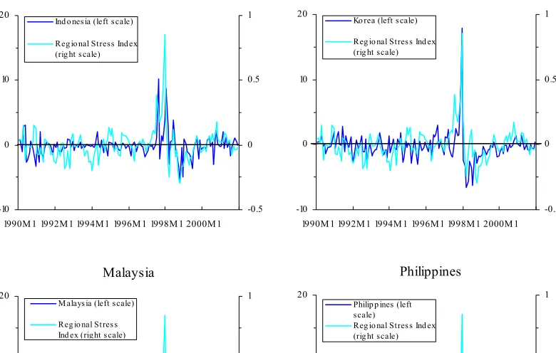
Negative EMPIs indicate speculators’ expectations of currency appreciation rather than depreciation. High EMPIs in some countries prior to the 1997 Asian crisis indicate that these countries had in fact been exposed to the danger of crisis but that attacks had been staved off. Figure 1 also shows the common or regional component of the EMPI across the six countries, the estimation of which is discussed directly below.
4.3 The Regional Stress Factor
The maximum likelihood estimates of the state space parameters and the implied level of common stress are displayed in Figure 1. The regional stress level is especially high during the height of the crisis, June1997 to January 1998. The index remains near zero or negative in most other periods except for a slight increase during the Mexican crisis. Negative values of the stress index may be interpreted as indicating regional optimism from the point of view of international investors.
The charts in Figure 1 and the estimation results in Table 1 reveal that the regional stress factor plays an important role in driving the exchange market pressure indices of all of the countries examined. In particular φ, the autoregressive parameter of the unobserved common factor, is statistically significantly different from zero and plausible in magnitude. The estimated γ(i) parameters, which measure the importance of common regional stress in driving the EMPI in each country, are in every case strongly significantly different from zero at conventional nominal test sizes. The degree of variation in each country’s EMPI explained by the regional stress factor ranges from 21 percent for Thailand, to 70 percent for the Philippines.
4.4 Analyzing the sources of vulnerability
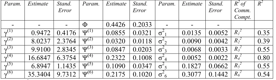
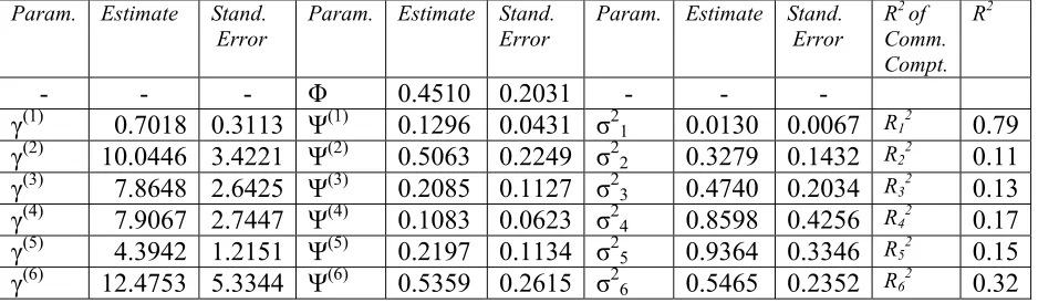
We considered a variety of macroeconomic and financial variables as potential drivers of the degree of vulnerability, including percentage monthly changes in the real (consumer price index-deflated) stock market index, the level of total foreign liabilities as a proportion of GDP, the ratio of M2 money supply to GDP (inverse velocity), and percentage monthly changes in the level of domestic credit outstanding in real terms. In order to obtain a measure of similarity in these macroeconomic fundamentals, we used the Kalman filtering method outlined above to extract a regional common factor for each of these series, and the results of this dynamic factor analysis are given in Tables 2-5.
Treasury rates).11 Gertler and Lown (2000) argue that a rise in the spread (and, hence, in the external costs of borrowing) reflects a lowering of the collateral value that borrowing firms can offer. In turn, this reduced collateral results from downgrading of growth prospects. Since exports to the United States play an important role in East Asian economic activity, it is not surprising that the prospect of a slowdown in the US reduces the net demand for East Asian currencies. Mody and Taylor (2002b) find that a rise in US high yield spread leads to a significant curtailment of capital flows to emerging markets (and, indeed, its influence overshadows that of US interest rates).
Having extracted the regional common factor of each of these series across the six countries concerned, we then regressed the common regional stress factor onto the current value and the first lagged value of each of the macro fundamental common factors. Interestingly, all of the current values of the macro common factors appeared significant in the regression, although of the lagged common factors, only the change in the real stock market index was significant. The resulting estimated regression equation was therefore of the form:
t t
t t
t
t 5
(1.8841) 4.8224 4
(0.2017) 0.4288 3
(0.1162) 0.2101 2
(2.7365) 6.6139 1
(1.4420) 3.3046 1
(1.4762)
5.2263 µ µ t-1 µ µ µ µ
κ =− − + + + +
R2=0.26, DW=1.17, Chow(>98)=0.3576 (28)
where figures in parentheses denote estimated standard errors and where:
κt = common regional stress index
µ1t = common factor of monthly log-change in real value of the stock market index µ2t = common factor of logarithm of ratio of total foreign liabilities to GDP
µ3t = common factor of logarithm of ratio of M2 to GDP
µ4t = common factor of monthly log-change in real value of domestic credit HYSt = US high-yield spread
µ5t = (∆ HYSt x µ4t)
R2 = coefficient of determination DW = Durbin-Watson statistic
Chow(>98) = p-value of a Chow test for a structural break in the parameters after 1998
It is interesting to note that similarity in financial indicators is capable of explaining 26 percent of the variation in the regional stress index, and that indicators such as the ratio of total foreign liabilities to GDP, inverse velocity and changes in the level of real domestic credit enter with significant and positive coefficients. Note also, that a test for a structural
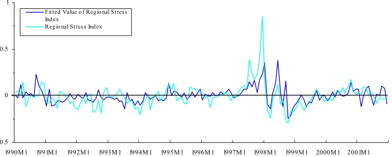
break after the crisis suggests no change and, hence, the same pattern of vulnerability continues. Most interestingly, the interaction of the change in real domestic credit and the US high-yield spread enters positively and significantly. Thus, to the extent that credit growth in excess of inflation implies a loose monetary policy, as suggested by Tanner (2001), and/or is associated with likelihood of unproductive investments, the implication is that such domestic vulnerability is aggravated by the joint effects of a larger premium being required by international investors for holding risky assets, and by the prediction of poorer export prospects on account of slower expected US growth which a rise in the high-yield spread predicts. The fitted values from this estimation seem to track well the actual values of the regional stress index (Figure 2 panel a).
One shortcoming of this estimated equation, however, is the evidence of first-order serial correlation, as shown by the low value of the Durbin-Watson statistic, even though we included lagged values of the macro fundamental variables. Accordingly, we re-estimated the equation with one lag of the dependent variable on the right-hand side. This led to the lagged change in the real stock market index and the inverse velocity factor becoming insignificant, so that the resulting equation was:
1
(0.0729) 0.5169 5
(1.7651) 5.1735 4
(0.0918) 0.2012 2
(2.3456) 5.6152 1
(1.3072)
3.4443 + + + + −
−
= t t t t t
t µ µ µ µ κ
κ
R2=0.43, DW=1.94, Chow(>98)=0.4662. (29)
The degree of variation in regional stress explained by the equation has now risen to 43 percent and the dynamic correspondence between the fitted estimates and the actual values of the regional stress index is now even better (Figure 2 panel b), and again there is no sign of a structural break post-1998. Again, we see that the interaction term involving the product of the US high-yield spread and changes in the real level of domestic credit enters strongly significantly.
In Figure 2 panel c we have graphed the contribution of the interaction term in equation (29) (i.e. 5.1735µ5t) together with the regional stress index itself: clearly, the interaction term tracks the regional stress index well, especially around the 1997-98 crisis period.
4.5 The dynamic interaction of regional stress and common macro fundamentals
to the macroeconomic and financial similarity variables, we were reluctant to include both changes in domestic credit and the interaction term in the same VAR since this would make interpretation of the impulse-response functions problematic because of the nonlinear
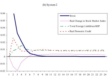
relationship between these two variables. Accordingly, we estimated two systems: System 1, which included the regional stress index (κt) and the regional common factors of the changes in the real stock market index (µ1t), of the ratio of total foreign liabilities to GDP (µ2t), and the interaction between changes in the high-yield spread and the common factor of changes in real domestic credit (µ5t); and System 2, which included κt, µ1t, µ2t and the regional common factor of changes in real domestic credit, µ4t.12
Using the Aikaike information criterion, we settled on a third-order VAR for both systems. We then used the estimated VARs to construct impulse-response functions.13 We have graphed the response of the regional stress index to shocks to itself and to each of the three macro similarity variables derived from Systems 1 and 2 in Figure 3. These impulse-response functions can in fact be interpreted as the impulse-response of regional vulnerability to innovations in each of the fundamentals variables since, by definition, movements in the regional stress index which are explained by movements in the fundamentals are in fact the same as movements in vulnerability.
Interestingly, the impulse-responses of regional stress with respect to shocks to itself and to µ1t and µ2t seem little affected by the choice of VAR and, moreover, each of the impulse-response functions show an interesting pattern capable of entirely intuitive interpretation. The impulse-response of the regional stress index to own shocks mean reverts toward zero with a half-life of between two and three months. Since this movement is conditional on holding the macro similarity variables constant, this may be interpreted as a measure of the degree to which pure market sentiment, independent of the fundamentals, affects the regional stress index.
The impulse response of regional stress (and hence vulnerability) to movements in the stock market index is also very interesting: although the effect for the first few periods is to reduce
12 In fact, we found that the impulse-response functions obtained with all the variables, including both µ4t and µ5t, in the VAR were qualitatively extremely similar to those we report below for the two separate systems, which is not surprising since µ4t and µ5t do not have a high degree of linear dependence. Nevertheless, we prefer to report the results obtained using the two systems, in order to make clear the interpretation of the impulse-response functions.
vulnerability—consistent with our single-equation regression results—the net long-term effect is in fact to raise regional vulnerability. As would be expected, an increase in total foreign liabilities as a proportion of GDP raises vulnerability in both the short run and the long run.
Shocks to the interaction between domestic credit and changes in the high-yield spread also tend to raise the vulnerability index in both the short run and the long run. Comparing Figures 3(a) and 3(b), however, it is interesting to note that shocks to the interactive term indicate a much more acute effect on regional vulnerability in the short run than do shocks to domestic credit alone.
4.6 The role of macro similarity in explaining individual country EMPIs
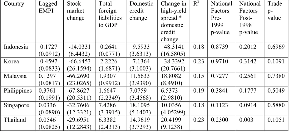
We next investigated the extent to which the common factors in the macro fundamentals are capable of explaining movements in individual country EMPIs. We did this by regressing the individual country EMPIs onto the same set of variables as in regression equation (28), except that the individual country lagged EMPI replaces the regional stress index. The results are given in Table 6. Interestingly, in most cases the variables enter with strongly significant coefficients which are the same sign as those reported in equations (28) or (29).
Columns 8 and 9 of Table 6 report the marginal significance level, or p-value, of an F-test of the significance of adding in the country-specific components of the macro fundamental variables into the regression, both for the post-1998 (i.e. post-crisis) period and for the pre-1999 period. In nearly every case, these p-values indicate that the national factors are insignificant in explaining movements in individual country EMPIs, although the marginal significance levels do appear to shrink post 1998, perhaps indicating a move towards greater importance of national factors. This is especially evident in the case of Thailand, which in fact has a p-value for the post-1998 period significantly less than 5 percent. Closer
examination of the Thai regression reveals that it is the national component of the change in real domestic credit that is strongly significantly different from zero, with a marginal
significance level of the t-ratio of the estimated coefficient of 0.0003. Testing for the significance of the remaining three national factors yielded a marginal significance level of 0.20.
Finally, we measured the importance of trade linkages in explaining individual country EMPIs, once the influence of macro similarity had been accounted for. Following Fratzscher (1999), the degree of trade integration of the country i with country j is measured as below (Fratzscher, 1999):
∑
∑
∑
× + ++=
.
d c ci c
c ji c ij c
id c
d c jd
c
ij X X
X X X
X X X Trade
i. . i.
The first term indicates the degree of competition of country j for home country i in the export market of commodity c, in the third market d. Third markets include industrialized countries (d: US, Europe and Japan), developing countries (d: Africa, Asia, Eastern Europe, Middle East and Western Hemisphere), and other regions. The larger the export market share of country j in region d, i.e. ( / .c)
d c jd X
X , and the higher the share for country i of total exports to that region d, i.e.(X c /Xi.)
id , the more severely will country i be affected by devaluation in country j. The second term measures the degree of bilateral trade between countries i and j, suggesting that country i will be affected more by a devaluation in country j if the volume of bilateral trade is greater between them. This variable was constructed on a monthly basis for each of the six countries under investigation, with respect to each of the other five countries, for our sample period. We then added the five trade linkage variables together for each country to provide and overall measure of trade linkage of each of the countries under examination with the other five countries over the sample period.14
In the final column of Table 6, we report the p-value resulting from a t-test of the significance of this variable when it is added into the EMPI regression for each of the individual countries, controlling for the international common components of the macro fundamental series. In each case, the marginal significance levels indicate that the variable is not significant at standard significance levels.
The fact that trade linkages do not appear significant in explaining movements in the EMPI over time should not, however, be taken as contradicting the findings of Glick and Rose (1999), who find that trade linkages are significant in explaining contagion. As noted earlier in our discussion, the “contagious crises” literature asks a different question from that posed in the present analysis, i.e. given that a crisis has occurred, who else is most likely to be affected? In the present study, we are primarily examining the vulnerability of a region to the occurrence of a crisis.
5. Conclusion
In this paper, we have focused on the vulnerability of a region to exchange rate crisis, rather than on explaining how that crisis is transmitted once it has occurred, which is the central focus of the “contagious crises” literature. Our aim has been to identify a set of underlying variables which contribute to that vulnerability, so that the analysis may ultimately be of use for policy purposes. Thus, our ultimate aim has been to contribute to an understanding of how crises may be prevented, rather than an understanding of how they spread.15
14 Trade data was obtained from the International Monetary Fund’s Direction of Trade Statistics. We are grateful to Jung Yeon Kim for help in constructing these indices.
In particular, we constructed a measure of regional financial stress using dynamic factor analysis which partitions the EMPIs of a group of countries into a common or regional component and a country-specific, idiosyncratic component. We have also shown how this regional stress index can be further partitioned into a component that is predictable given the underlying regional measures of macro and financial similarity (leading to a measure of regional vulnerability) and a part that is unexpected based on the fundamentals (a residual measure that could be interpreted as regional contagion). Our methodology was applied using data from January 1990 to December 2001 for six Asian countries most severely affected by the1997 currency crisis: Thailand, Indonesia, the Philippines, Malaysia, Singapore and Korea.
To summarize our empirical results briefly, regional vulnerability appears to arise in the context of regional accumulation of foreign liabilities and the rapid growth of domestic credit and stock markets. Global, or “monsoonal,” effects are proxied by the rise in risk premia in financial markets, which signal also a slowdown in US growth, amplifying the vulnerabilities on account of credit growth. There is no evidence for a structural change in the sources of vulnerability following the Asian crisis. Our results also suggest that individual country EMPIs are also explained by the common regional factors that drive the level of regional vulnerability. Country-specific factors have played almost no role, with the exception of Thailand, and to a lesser extent for Singapore, both in the post-crisis period.
Table 1: State Space Parameter Estimation Results: Exchange Market Pressure Index
Param. Estimate Stand.
Error Param. Estimate Stand. Error Param. Estimate Stand. Error R
2 of
Common Component
R2
- - - φ 0.1846 0.5143 - - -
γ(1) 0.4699 0.1034 Ψ(1) 0.1151 0.3045 σ21 2.8836 1.0032 R12 0.29
γ(2) 12.4633 2.3254 Ψ(2) 0.1088 0.2098 σ22 4.8749 1.9632 R22 0.33
γ(3) 10.5574 2.1194 Ψ(3) 0.4059 0.1174 σ23 2.1963 0.9053 R32 0.40
γ(4) 5.0734 1.0043 Ψ(4) 0.5205 0.1947 σ24 1.8764 0.8176 R42 0.70
γ(5) 3.7972 0.8521 Ψ(5) 0.1430 0.0221 σ25 1.4137 0.6542 R52 0.25
γ(6) 40.5731 3.8862 Ψ(6) 0.3300 0.1241 σ26 3.1115 0.6658 R62 0.21
Note: R2
i denotes the coefficient of determination in a regression of the country variable onto the extracted
common factor for country i, with 1=Indonesia, 2=Korea, 3=Malaysia, 4=Philippines, 5=Singapore, 6=Thailand.
Table 2: State Space Parameter Estimation Results: Real Stock Market Changes
Param. Estimate Stand. Error
Param. Estimate Stand. Error
Param. Estimate Stand. Error
R2 of
Comm. Compt.
R2
- - - Φ 0.4426 0.2033 - - -
γ(1) 0.9472 0.4176 Ψ(1) 0.0855 0.0321 σ21 0.0135 0.0052 R12 0.35
γ(2) 8.0237 2.3764 Ψ(2) 0.0320 0.0118 σ22 0.0090 0.0042 R22 0.39
γ(3) 9.9100 2.8345 Ψ(3) 0.0847 0.0203 σ23 0.0068 0.0033 R32 0.55
γ(4) 16.6847 6.3754 Ψ(4) 0.2322 0.1008 σ24 0.0052 0.0022 R42 0.80
γ(5) 6.8947 1.1435 Ψ(5) 0.1090 0.0347 σ25 0.1827 0.0662 R52 0.55
γ(6) 35.3404 9.7312 Ψ(6) 0.2175 0.1020 σ2
6 0.3077 0.1442 R62 0.54
Note: R2i denotes the coefficient of determination in a regression of the country variable onto the extracted
[image:26.612.83.556.449.587.2]Table 3: State Space Parameter Estimation Results: Ratio of Total Foreign Liabilities to Nominal GDP
Param. Estimate Stand.
Error Param. Estimate Stand. Error Param. Estimate Stand. Error R
2 of
Comm. Compt.
R2
- - - Φ 0.6034 0.2334 - - -
γ(1) 1.7771 0.5621 Ψ(1) 0.2152 0.1123 σ21 0.2123 0.1003 R12 0.29
γ(2) 3.2213 1.1331 Ψ(2) 0.2981 0.1432 σ22 0.2621 0.1326 R22 0.26
γ(3) 4.1239 2.0003 Ψ(3) 0.2315 0.1183 σ23 0.0981 0.0224 R32 0.23
γ(4) 8.9991 3.1123 Ψ(4) 0.2411 0.1221 σ24 0.0991 0.0221 R42 0.11
γ(5) 5.6673 2.1561 Ψ(5) 0.2318 0.1010 σ25 0.4146 0.2153 R52 0.05
γ(6) 9.8899 4.6391 Ψ(6) 0.3159 0.1235 σ26 0.4733 0.2236 R62 0.20
Note: R2
i denotes the coefficient of determination in a regression of the country variable onto the extracted
[image:27.612.85.554.463.600.2]common factor for country i, with 1=Indonesia, 2=Korea, 3=Malaysia, 4=Philippines, 5=Singapore, 6=Thailand.
Table 4: State Space Parameter Estimation Results: Changes in Real Domestic Credit
Param. Estimate Stand.
Error Param. Estimate Stand. Error Param. Estimate Stand. Error R
2 of
Comm. Compt.
R2
- - - Φ 0.4510 0.2031 - - -
γ(1) 0.7018 0.3113 Ψ(1) 0.1296 0.0431 σ21 0.0130 0.0067 R12 0.79
γ(2) 10.0446 3.4221 Ψ(2) 0.5063 0.2249 σ22 0.3279 0.1432 R22 0.11
γ(3) 7.8648 2.6425 Ψ(3) 0.2085 0.1127 σ23 0.4740 0.2034 R32 0.13
γ(4) 7.9067 2.7447 Ψ(4) 0.1083 0.0623 σ24 0.8598 0.4256 R42 0.17
γ(5) 4.3942 1.2151 Ψ(5) 0.2197 0.1134 σ25 0.9364 0.3346 R52 0.15
γ(6) 12.4753 5.3344 Ψ(6) 0.5359 0.2615 σ26 0.5465 0.2352 R62 0.32
Note: R2
i denotes the coefficient of determination in a regression of the country variable onto the extracted
Table 5: State Space Parameter Estimation Results: Ratio of M2 to GDP
Param. Estimate Stand.
Error Param. Estimate Stand. Error Param. Estimate Stand. Error R
2 of
Comm. Compt.
R2
- - - Φ 0.6422 0.2270 - - -
γ(1) 0.8156 0.3416 Ψ(1) 0.2153 0.1013 σ21 0.0177 0.0061 R12 0.73
γ(2) 8.1952 3.9228 Ψ(2) 0.5155 0.2413 σ22 0.3142 0.1553 R22 0.41
γ(3) 8.1265 3.8873 Ψ(3) 0.2144 0.1143 σ23 0.4521 0.2152 R32 0.66
γ(4) 6.4432 2.9853 Ψ(4) 0.1432 0.0631 σ24 0.7861 0.3734 R42 0.73
γ(5) 2.1123 1.0338 Ψ(5) 0.2248 0.1133 σ25 0.8355 0.3124 R52 0.21
γ(6) 16.8913 4.3899 Ψ(6) 0.6349 0.2816 σ26 0.5671 0.2445 R62 0.67
Note: R2
i denotes the coefficient of determination in a regression of the country variable onto the extracted
common factor for country i, with 1=Indonesia, 2=Korea, 3=Malaysia, 4=Philippines, 5=Singapore, 6=Thailand.
Table 6: Individual Country EMPI Regressions
Country Lagged EMPI
Stock market change
Total foreign liabilities to GDP
Domestic credit change
Change in high-yield spread * domestic credit change
R2 National
Factors Pre-1999 p-value
National Factors Post-1998 p-value
Trade p-value
Indonesia 0.1727
(0.0912) -14.0331 (6.4432) 0.2641 (0.0771) 9.5933 (3.6313) 48.3141 (16.5805) 0.18 0.8739 0.2012 0.6969
Korea 0.4597
(0.0833) -66.6453 (26.1594) 2.2226 (1.6871) 7.1364 (3.1003) 38.3392 (20.7661) 0.23 0.9710 0.3142 0.1091
Malaysia 0.1297
(0.0817) -66.2690 (23.0265) 1.9307 (0.9912) 11.5633 (3.9390) 18.8082 (8.4910) 0.15 0.7277 0.2561 0.7380
Philippines 0.3761 (0.1991)
-67.8627 (20.5311)
1.6647 (2.2349)
7.0759 (3.4568)
6.5373 (2.9810)
0.19 0.3841 0.1777 0.5049
Singapore 0.0336
(0.0890) -32.7606 (12.3321) 7.4286 (3.3915) 18.1095 (5.1403) 10.0356 (4.05299) 0.18 0.1123 0.0914 0.5880
Thailand 0.0546
(0.0825) -29.6951 (12.2843) 6.3382 (2.4313) 14.9619 (3.7293) 20.4199 (9.1238) 0.23 0.2300 0.003 0.1051
[image:28.612.84.550.353.567.2]Figure 1. Exchange Market Pressure Index Indonesia -10 0 10 20
1990M 1 1992M1 1994M1 1996M 1 1998M 1 2000M1 -0.5 0 0.5 1
Ind o nes ia (left s cale)
Reg io nal Stress Index (rig ht s cale)
Korea
-10 0 10 20
1990M 1 1992M 1 1994M 1 1996M1 1998M1 2000M 1 -0.5 0 0.5 1
Ko rea (left s cale) Reg io nal Stres s Ind ex (rig ht scale)
Malaysia
-10 0 10 20
1990M 1 1992M1 1994M1 1996M 1 1998M 1 2000M1 -0.5 0 0.5 1
M alays ia (left scale) Reg io nal Stres s Ind ex (right s cale)
Philippines
-10 0 10 20
1990M 1 1992M 1 1994M 1 1996M1 1998M1 2000M 1 -0.5 0 0.5 1
Philip p ines (left scale)
Reg io nal Stres s Ind ex (rig ht scale)
Singapore -20 -10 0 10 20 -1 -0.5 0 0.5 1
Sing ap o re (left s cale) Reg io nal Stres s Ind ex (rig ht s cale)
Thailand -10 0 10 20 -0.5 0 0.5 1
Thailand (left s cale)
Figure 2. Explaining Common Regional Stress
(a) Fitted Value of Regional Stress Index
-0.5 0 0.5 1
1990M 1 1991M1 1992M1 1993M 1 1994M 1 1995M1 1996M 1 1997M 1 1998M1 1999M 1 2000M 1 2001M1
Fitted Value o f Reg io nal Stres s Ind ex
Reg io nal Stres s Ind ex
(b) Fitted Value of Regional Stress Index with Lagged Dependent Variable
-0.5 0 0.5 1
1990M 1 1991M1 1992M1 1993M 1 1994M 1 1995M1 1996M 1 1997M 1 1998M1 1999M 1 2000M 1 2001M1
Fitted Value o f Reg io nal Stress Index with Lag g ed Dep end ent Variab le
Regio nal Stress Ind ex
(c) Contribution of Interaction Term in Explaining Regional Stress Index
-0.5 0 0.5 1
1990M 1 1991M1 1992M1 1993M 1 1994M 1 1995M1 1996M 1 1997M 1 1998M1 1999M 1 2000M 1 2001M1
Co ntrib ution of Interaction Term in Exp laining Reg io nal Stress Ind ex
Figure 3. Impulse Response Functions of Regional Stress
(a) System 1
-0.02 -0.01 0 0.01 0.02 0.03 0.04 0.05 0.06
1 2 3 4 5 6 7 8 9 10 11 12 13 14 15 16 17 18 19 20 21 22 23 24 Stress
Real Change in Stock Market Index T otal Foreign Liabilities/GDP
Change in US High Yield Spread x Change in Real Domestic Credit
(b) System 2
-0.02 -0.01 0 0.01 0.02 0.03 0.04 0.05 0.06
1 2 3 4 5 6 7 8 9 10 11 12 13 14 15 16 17 18 19 20 21 22 23 24 Stress
Real Change in Stock Market Index
T otal Foreign Liabilities/GDP
References
Agénor, Pierre-Richard, Marcus Miller, David Vines, and Axel Weber (eds.) (1999) The Asian Financial Crisis: Causes, Contagion and Consequences. Cambridge, New York and Melbourne: Cambridge University Press.
Bank for International Settlements (1998) Annual Report. Basle, Switzerland: Bank for International Settlements.
Bordo, Michael and Antu Murshid (2002) “Globalization and Changing Patterns in the International Transmission of Shocks in Financial Markets,” National Bureau of Economic Research Working Paper 9019, Cambridge MA.
Boyer, Brian H., Michael S. Gibson, and Mico Loretan (1999) “Pitfalls in Tests for Changes in Correlations,” International Finance Discussion Paper 597R, Federal Reserve Board, Washington D.C.
Calvo, Guillermo A., and Enrique Mendoza (2000) “Rational Contagion and the Globalization of Securities Markets,” Journal of International Economics 51: 79-113.
Campa, Jose and Kevin Chang (1996) “Arbitrage-Based Tests of Target-Zone Credibility: Evidence from ERM Cross-Rate Options,” American Economic Review 86: 726-740.
Caramazza, Francesco, Luca Ricci, and Ranil Salgado (2000) “Trade and Financial Contagion in Currency Crises,” International Monetary Fund Working Paper WP/00/55, Washington D.C.
Chinn, Menzie D. (1999) “On the Won and Other East Asian Currencies,” International Journal of Finance and Economics 4: 113-127.
Chinn, Menzie D. (2000) “Before the Fall: Were East Asian Currencies Overvalued?” Emerging Markets Review 1: 101-126.
Chinn, Menzie D., and Michael P. Dooley (1997) “Asia–Pacific Capital Markets:
Measurement of Integration and the Implications for Economic Activity,” in Takatoshi Ito and Anne O. Krueger (eds.) Regionalism Versus Multilateral Trading Arrangements. Chicago: Chicago University Press: 169-196.
Chinn, Menzie D., and Michael P. Dooley (1999) “International Monetary Arrangements in the Asia-Pacific Before and After,” Journal of Asian Economics 10: 361-84.
Claessens, Stijn, and Kristin J. Forbes (eds.) (2001) International Financial Contagion. Boston: Kluwer Academic Publishers.
Corsetti, Giancarlo, Marcello Pericoli, and Massimo Sbracia (2002) “Some Contagion, Some Interdependence: More Pitfalls in the Tests of Financial Contagion.” Available at
www.econ.yale.edu/~corsetti/
Corsetti, Giancarlo, Paolo Pesenti, and Nouriel Roubini (1999) “The Asian Crisis: An Overview of the Empirical Evidence and Policy Debate,” in Agénor et al. (1999): 127-163.
Cuthbertson, Keith, Stephen G. Hall and Mark P. Taylor (1992) Applied Econometric Techniques. Ann Arbor: University of Michigan Press, 1992.
Dooley, Michael P. (1997) “A Model of Crises in Emerging Markets.” International Finance Discussion Paper 630, Board of Governors of the Federal Reserve System, Washington, DC.
Edwards, Sebastian (2000a) “Contagion,” World Economy 23: 873-900.
Edwards, Sebastian (2000b) “Interest Rates, Contagion and Capital Controls,” National Bureau of Economic Research Working Paper 7801, Cambridge MA.
Eichengreen, Barry, Andrew Rose, and Charles Wyplosz (1996) “Contagious Currency Crises,” Scandinavian Economic Review 98(4): 463-484.
Eichengreen, Barry, Galina Hale, and Ashoka Mody (2001) “Flight to Quality: Investor Risk Tolerance and the Spread of Emerging Market Crises,” in Claessens and Forbes (2001).
Engle, Robert F. and Mark F. Watson (1981) “A One-Factor Multivariate Time-Series Model of Metropolitan Wage Rates,” Journal of the American Statistical Association 76: 774-781.
Flood, Robert, and Nancy Marion, Nancy (1999) “Perspectives on the Recent Currency Crisis Literature,” International Journal of Finance and Economics 4: 1-26
Forbes, Kristin J. (2001) “Are Trade Linkages Important Determinants of Country Vulnerability to Crises?” National Bureau of Economic Research Working Paper 8194, Cambridge MA.
Forbes, Kristin J. and Roberto Rigobon (2001) “Measuring Contagion: Conceptual and Empirical Issues,” in Claessens and Forbes (2001).