A quest for the best automated tests : Estimating software reliability based on Spec Explorer's on the fly test results

UNIVERSITEIT TWENTE

Master thesis

A quest for the best automated tests

Estimating software reliability based on Spec Explorer’s on-the-fly test results

May, 2016

Candidate: Jenny den Ouden

Graduation committee: dr. M.I.A. Stoelinga (first supervisor)

ir. R. Kherrazi (external supervisor) M. Gerhold, MSc

prof. dr. J.C. van de Pol

Abstract

Spec Explorer on-the-fly testing does not provide any indication of coverage or reliability regarding the system under test, or say whether testing can be stopped. This means that testing is useful for fault discovery, but there is no way of knowing whether you’ve tested enough. As a step towards remedying this, this thesis presents a tool that estimates the reliability of a system under test after Spec Explorer on-the-fly testing has been applied to it. The on-the-fly test results are used to construct a usage and a testing chain, from which the discriminant, reliability, and mean time between failures can be estimated. The tool is applied to two simple examples. The results that are obtained are used to draw conclusions about the usefulness of the tool, as well as for providing suggestions for tool improvements and possible future research.

Acknowledgements

I want to thank Mari¨elle and Rachid for their guidance and supervision. I am also grateful to Marcus for all his feedback and help. I want to thank Jaco for agreeing to be in the graduation committee, and for his feedback and encouragement.

Contents

1 Introduction 3

2 Problem statement 4

3 Background 6

3.1 Usage and testing chains . . . 7

3.2 Discriminant . . . 10

3.3 Reliability . . . 14

3.4 Mean time between failures . . . 15

4 Post processer tool 17 4.1 Purpose . . . 17

4.2 Using the tool . . . 18

4.2.1 Important model properties . . . 18

4.2.2 Introducing probabilities into the model . . . 18

4.2.3 Using the tool . . . 19

4.3 Tool structure . . . 19

4.4 Extendability . . . 22

5 Experiments 22 5.1 Simple example model . . . 24

5.2 Simplified case study . . . 28

6 Discussion 34 6.1 Discriminant . . . 34

6.2 Reliability . . . 37

6.3 Mean time between failures . . . 40

6.4 Limitations and future work . . . 43

7 Conclusion 44

1

Introduction

In this thesis, commissioned by technical consultancy company Nspyre, we apply a reliability es-timation technique from theory to model based software testing in practice. In our case, we add reliability measures as described in [22], and a manner to include usage probabilities in models, to the on-the-fly testing functionality in model based testing tool Spec Explorer. This results in an estimate of the reliability of the system under test: a measure that is currently not available in the Spec Explorer tool. We have also briefly studied a set of other model based statistical testing tools, but found that reliability estimation is not much applied in general. We would like to take some steps towards fixing this.

Anyone who has ever done any programming, should also have carried out some software tests, to check whether their code does what they meant it to do. And all these people will know that testing is a very time consuming process (not to mention, rather boring). However, testing is also an essential part of software development, and since nearly everything contains technology of some kind, refraining from testing (and consequently missing implementation errors) could have very serious consequences. I would rather not be in an airplane, or even a car, when the entire system crashes and the vehicle is uncontrollable.

Thus, software testing is paramount, and it is also a lot of work. A solution for this is auto-mated testing, which happens in model based testing (MBT). The idea behind MBT is that you translate the requirements of the system you want to test into a model, from which a MBT tool can automatically generate and run tests. Model based testing has some startup costs in creating the model. However, due to the formal, unambiguous definition of the model, defects in the system can already be discovered during the creation of the model [9]. Additionally, the automated generation and execution of the tests saves you enough time for it to be worth the initial investment [15], not to mention that, when the application and the test evolve, it is often sufficient to update the model incrementally with the corresponding changes [9].

According to [1], model based testing consists of four steps: modeling the system; generating tests from that model; running the tests against an implementation; and comparing the results to the results that were expected. During this final step, the tester should decide whether or not to stop testing. To support this decision, the tester can, for instance, compute the reliability of the system.

The reliability, which is defined here as the probability that a single, randomly selected test is executed without the occurrence of any failure, can not only be used as (part of a) stopping criterion for test generation, but it can also serve as an estimate of the system under test’s quality. Neither of these two functions are available in Spec Explorer at the moment.

Finding a useful reliability measure is not easy; there is a real need for metrics related to soft-ware and system reliability [5, 18]. In many cases, coverage is used as a reliability measure [2]. The idea behind this is that, once a test case is passed, the coverage points visited by the test suite are reliable. The percentage of coverage points is directly translated to a reliability score. This technique is, for instance, applied in [4, 7, 18].

test-ing is done by sampltest-ing the input space of a model, possibly accordtest-ing to a usage model [15]. Such a strategy is also applied by Spec Explorer on-the-fly testing [19]. That paper suggests that transition selection is not purely random, but it also emphasizes that the algorithm stochastically samples the state space, implying that Spec Explorer’s on-the-fly testing is suitable for reliability estimation.

In order to apply the reliability estimate we selected, we need to know the usage model (or uni-form model) that was used for test generation, as well as the on-the-fly test results. Spec Explorer provides both these items as exploration files. We developed a tool that takes these outputs and uses them to estimate the reliability of the system under test. This post-processor tool was used in a set of experiments to study the way the reliability reacts to failures. Based on the results that were obtained, we indicate some limitations of the tool, and the method, as well as recommending some future work.

In section 2, we specify the problem statement. Section 3 of this document explains the afore-mentioned reliability measures [22], and shows how they are computed. In section 4 we describe the structure of the tool. Section 5 describes the experiments we carried out, the results to which are discussed in section 6. Finally, we recap and conclude the thesis in section 7.

2

Problem statement

Nspyre, the company for which I carry out this research, is a Dutch company with its focus on tech-nology. There are several Competence Units within Nspyre, one of which is ’Test and Integration’. This unit focuses on providing software testing for (large) companies, and they regularly use Spec Explorer, a model based testing tool, to achieve this.

The goal of this thesis is to provide a reliability estimate for the Spec Explorer tool, and to try it out on some small examples to see what insights it provides, and to see whether it will be useful for Nspyre. This problem statement gives rise to three follow-up questions: why do we want a reli-ability estimate, why do we want to use Spec Explorer, and which method will we use to estimate the reliability?

Motivation

First of all, we asked why a reliability estimate could be useful in this context. The purpose of testing is to discover as many failures as possible early on in the development process. Since de-tecting costs early on is considerably cheaper than dede-tecting them later (for example after system deployment) [13], making sure that you catch as many failures as possible in the testing stage will save testers and companies both time and money.

An indication of the system’s reliability can provide some trust in the implementation under test, and can serve as a stopping criterion for testing. This criterion could be used in two ways: the tester can consider the reliability estimate and use it to decide whether or not to stop testing; or the reliability estimate can be fed to the testing tool, which can make the decision to stop or continue testing.

The best we can do is estimate the reliability.

Tool choice

The second question was why we want to use Spec Explorer. This tool is Nspyre’s preferred tool, for several reasons. First of all, the company has a lot of experience with the tool [16, 17]. The employees are used to working with Spec Explorer, and switching to another tool would require a significant investment of time and money. Second of all, the tool is free. It only requires Visual Studio to run, so it is also accessible for Nspyre’s customers. Thirdly, Spec Explorer is suitable for embedded software, which is what most of the customers want to have tested. Additionally, the tool has a set of advanced features, such as model-slicing, non-determinism and online testing, and it is well documented.

However, there is no way to estimate the reliability of a system after it has been tested with Spec Explorer [18], particularly in on-the-fly testing, there is not even an indication of the percentage of state or transition coverage. In fact, in several Spec Explorer papers, the lack of reliability metrics (both in Spec Explorer and in model based testing in general) is lamented. Spec Explorer seems geared towards coverage as a reliability metric, but the authors acknowledge that this might be difficult to achieve when dealing with nondeterminism [18, 20, 21].

There are other model based testing tools that do provide some reliability measure. The most interesting one is the approach proposed by MaTeLo [14]. MaTeLo is a high-end test tool following the model based testing approach, designed for testing complex information systems and embed-ded systems. It can also generate tests based on a usage model. According to [6] their reliability measure will be implemented into the MaTeLo tool, but we have not found any evidence of this in the tool’s manual. Additionally, MaTeLo is a commercial tool, which would result in additional costs for Nspyre.

A second alternative model based testing tool is JUMBL, a tool which can also generate tests based on a usage model [12]. As opposed to MaTeLo and Spec Explorer, JUMBL works with a command line interface, which makes operating it less intuitive than operating Spec Explorer. JUMBL provides an indication of system reliability, which is computed according to [8].

So, with respect to relability measures, these two tools have some shortcomings. MaTeLo’s reliability has not been implemented, and JUMBL’s reliability does not take the achieved coverage into account: the coverage has no effect on the reliability value that is estimated. In this thesis, we will try to remedy these shortcomings, or suggest improvements that will better them in a future version of the tool.

These two tools are also lacking some functionality that Spec Explorer does have. First of all, Spec Explorer is able to deal with non-deterministic systems, while JUMBL and MaTeLo are not. Additionally, Spec Explorer allows for both online and offline test generation, whilst JUMBL and MaTeLo can only do offline generation. Thirdly, Spec Explorer is very suitable for testing com-plex models. Its modeling language is an extension of C#, and there are several constructs, such as model slicing, data abstraction, and model composition, that support complex modeling and reduce the state space explosion problem. The other two tools do not provide these, or similar options. Lastly, Spec Explorer is extendable by users, which allows for useful adaptations of the tool [3], [12].

An in-depth comparison of the available statistical model based testing tools is outside the scope of this thesis, but based on this short comparison, neither of the alternative tools warrant a switch for the entire competence unit. Instead, our goal is to estimate the reliability of a system after it has been tested with Spec Explorer. For this thesis, we will limit the testing to online (on-the-fly) testing.

Reliability estimation method

We would like to extend Spec Explorer with a reliability measure. But the question remains: which one is suitable? A study of all possible reliability measures is outside the scope of this thesis. There-fore, we will select from four options that came up during literature review: LeGuen [6], Miller [8], Sayre [11], and Whittaker [22]. Due to time constraints we decided not to find any additional reliability estimation methods.

Out of these four techniques, we are most familiar with Sayre, and Whittaker. LeGuen’s work is based on these two techniques, so it could be interesting. However, it is also very complex. We decided to drop this technique for now, but we should definitely keep it in mind for future work.

The Sayre method seems interesting, but when we studied it in detail, some things remained unclear with regard to the computation algorithm. It would take considerable time to discover the correct configuration. For this reason, we have decided to drop the Sayre technique.

When considering the remaining two techniques, our preference is to use the Whittaker mea-sures. This is for two reasons: first of all, we are more familiar with the Whittaker reliability measures, and second of all, they are slightly more recent than the Miller ones.

In this thesis, we want to see how the quality of Spec Explorer on-the-fly test sets, as well as the quality of the system under test, can be quantified in a way that is useful for Nspyre. For this purpose, we have developed a post-processing tool, which takes Spec Explorer’s on-the-fly testing results and computes the reliability of the system based on these, as proposed by Whittaker [22].

Next, we investigate how useful these Whittaker measures are. The post-processing tool will be tried on a small example, and on a simplified Nspyre case study, to see how it performs and what insights it gives. Based on these results, we will indicate some limitations of the tool, as well as propose possible future extensions.

3

Background

In this section we will describe the reliability measures introduced by Whittaker in [22]: discrimi-nant, reliability, and mean time between failures. We will use a small example to show how each of these measures is computed. In section 5 we apply our tool, which computes all three measures, to several test sets.

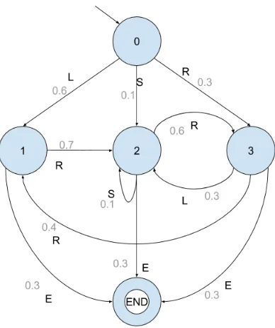
Figure 1: Example usage chain

3.1

Usage and testing chains

The basis for the techniques presented in [22] lies in the construction of two different models: the usage, and the testing chain. In the usage chain (definition 1), transitions are labeled with actions from the input domain of the software. These transitions are annotated with probabilities according to a usage model, or a uniform distribution if there is no information regarding the system’s use. System logs from a prototype or prior version of the software, for example, may be used to estimate the probabilities.

Definition 1 Ausage chain (or usage model) is a 6-tuple (S, sinit, Sfinal, A, C, P).

• S is a non-empty, finite set of states, withsinit∈S as exactly one initial state,

• Sfinal ⊆S is the non-empty set of final states,

• A is a non-empty finite set of actions,

• C⊆ {S×A×S}is the set of transitions,

• P :S×A×S→[0,1], is a usage probability, such that∀i∈S: (P

k∈A,j∈S P(si, ak, sj) = 1),

Definition 2 Atest for a usage chainU = (S, sinit, Sfinal, A, C, P) is a sequence of transitions

{(s0, a0, s1)(s1, a1, s2)...(sn, an, sn+1)}

where s0 = sinit, sn+1 ∈ Sfinal, and si ∈ S ∪Serror, for i = 0, ..., n, and where Serror is a set

of error states.

Testing chains (definition 3) are constructed during the testing process. The initial chain is a copy of the usage chain, with all probabilities set to 0. For each test sequence that is executed, the number on each transition is incremented when that transition is carried out. Transition probabilities can be determined by normalizing these numbers.

Definition 3 A testing chain (or testing model) is a 6-tuple (S, sinit, Sfinal, A, C, F), based on a

set of tests O.

• S is a non-empty, finite set of states, withsinit as exactly one initial state,

• Sfinal ⊆S is a non-empty, finite set of final states,

• A is a non-empty, finite set of actions,

• C⊆ {S×A×S}, is a set of transitions,

• F :S×A×S →Nis the frequency with which this transition has been crossed in test set O,

If failures occur, they need to be incorporated into the testing chain. To this end, a new failure state is introduced, with an incoming edge numbered 1, which can again be incremented, should the failure occur more often. If it is a catastrophic failure, the system moves into the terminal state (a transition from the error state to the terminal state is added). Otherwise, a transition is added to the state from which the system continues. These edges are also numbered 1, and can be incremented later.

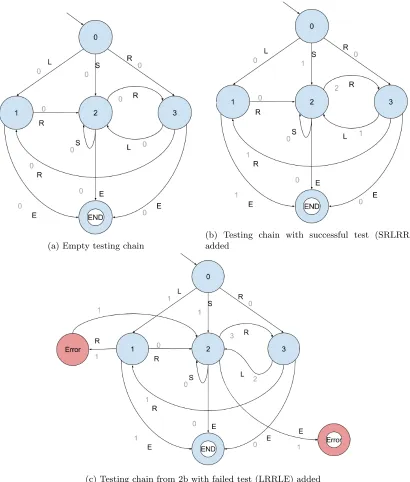
Construction of the testing chain is illustrated in figure 2. Figure 2a shows the initial testing chain: a copy of the usage chain, where the probabilities are replaced by frequencies, which are initialized at 0. Figure 2b shows the same testing chain after one test has been incorporated in the chain. This test is SRLRRE. It was successful, which means that all transitions succeeded and no errors need to be introduced. Figure 2c shows how failures are introduced into the chain. We consider a test LRRLE, which contains two failures. The first is a non-terminal failure in the second transition (R). The testing chain shows that an error state is introduced that is reached with R. Because this failure is not terminal, a transition from the error state to state 2, from which the sys-tem continues. The rest of the test is included in the chain, until we reach the final transition (E). This transition causes a terminal failure: the system cannot continue and the test is terminated. The image shows an accepting error state that is reached by E. There are no outgoing transitions from this state.

(a) Empty testing chain

(b) Testing chain with successful test (SRLRRE) added

(c) Testing chain from 2b with failed test (LRRLE) added

Whenever the system is updated (to fix bugs), the testing chain can either be reset, or left intact. This results in two possible testing chains that can be constructed: a chain over the testing of the current system, and a chain over the complete testing process. The first can be used to estimate the current reliability, whereas the second could be used to study the failure identification rate. If no errors occur, the testing chain will eventually converge to the usage chain.

In our tool, we will only use the first type of testing chain.

Now that we have constructed this testing chain, we want to use it to say something about the system’s reliability. The idea is that the more similar the two chains (usage model (U) and testing chain (T)) are, the more reliable the system is. U and T are regarded as equivalent when they are indistinguishable sequence generators, i.e. when given a sufficiently large test set, it is very difficult to determine if it was generated from U or from T. This is where the discriminant comes in.

3.2

Discriminant

In the previous section we mentioned that the similarity between the usage chain and the testing chain is a useful measure. However, we have not yet said anything about determining the level of similarity between the two chains.

The log likelihood ratio [10, 22] known as discriminant is used to measure how two stochastic processes relate to each other. If two stochastic processes tend to converge towards each other, the value of the discriminant approaches zero. Only if both are the same, the value is zero. Since usage chain U and testing chain T converge, the value of their discriminant approaches zero.

We calculate the discriminant according to the following equation (equation 1).

D(U, T) = Σ(i,j)πi∗pij∗log2

pij

ˆ

pij

(1)

Hereπis the stationary distribution of U,pij is the probability of a transition from i to j in U, and

ˆ

pij is the corresponding probability in T.

In the above formula, an error occurs in two cases: whenpij= 0 and when ˆpij= 0. In practice,

this means that we should only consider the transitions that occur with a probability larger than 0 in the usage chain. This also means that transitions to error states are not directly included in the computation. Their effect takes place in the testing chain probabilities from a state that is the source of a faulty transition: a fraction of outgoing transitions is siphoned away to an error state, and is not considered in regular state discriminant computations.

Additionally, we can only compute the discriminant once all these transitions that occur in the usage chain, occur at least once in the testing chain.

We will explain this formula by applying it to the example in figure 1, extended with a transi-tion from the end state to the initial state (state 0). We need to make this adjustment because we are using online testing, which does not have a stopping criterion (at least, not in Spec Explorer). This means that, when one test is completed, Spec Explorer will start from the initial state and generates a new test.

Transition Probability Frequency Relative frequency

0→1 0.6 4 0.444

0→2 0.1 2 0.222

0→3 0.3 3 0.333

1→2 0.7 3 0.375

1→4 0.3 5 0.625

2→2 0.1 1 0.077

2→3 0.6 9 0.692

2→4 0.3 3 0.231

3→1 0.4 4 0.333

3→2 0.3 7 0.583

3→4 0.3 1 0.083

Table 1: Relative frequencies after nine tests on example 1

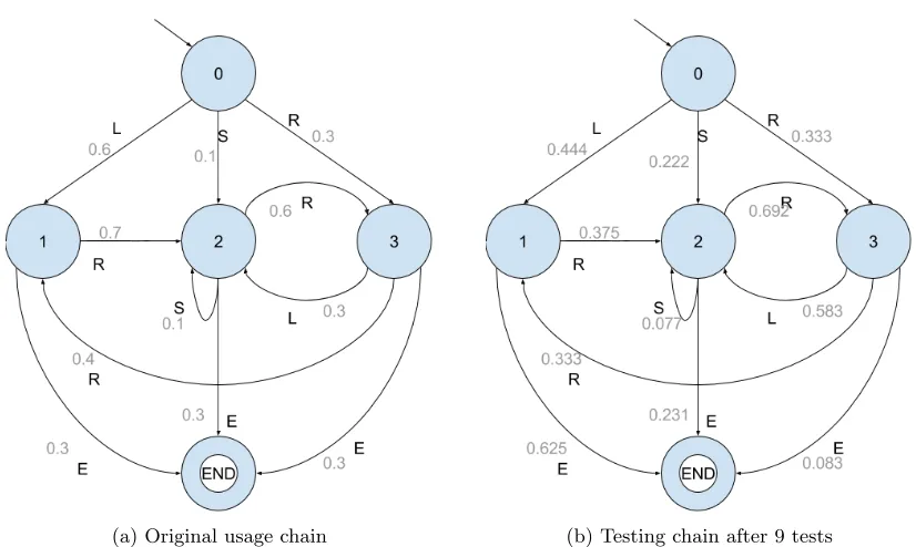
of 9 tests: SRLRRE, RLRRRRRE, LE, LE, RLSRLE, LRRLE, LRE, SRLRLRRE, RE. Table 1 summarizes the absolute and relative frequencies of each of the transitions. Figure 3 displays the relative frequencies visually, and compares them to the original usage model.

At this point, we can compute the discriminant. If we compute an updated discriminant value after each new test, we can plot the discriminant over time. When the testing chain grows quite similar to the usage chain i.e. the test history reflects the actual usage pattern, the value of D (U, T) becomes very small. Whenever a failure occurs the value of D (U, T) increases, so additional tests are required for minimizing that effect.

In order to compute the discriminant we need the stationary distribution of our model. The compu-tation of the scompu-tationary distribution is elaborated on in appendix A. The result of this compucompu-tation is shown in equation 2.

              

π0= 0.1875 π1= 0.1916

π2= 0.2357 π3= 0.1977

π4= 0.1875

(2)

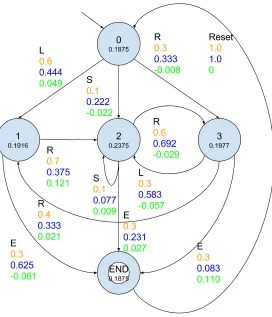
For clarity, we will display the computation of the discriminant in a table (Table 2), as well as in a figure (Figure 4). This table contains a column for each element in equation 1. Because the equation is a sum, we also use a column ”partial discriminant”. This column shows the partial sum for each transition. Finally, these partial discriminants are summed to find the discriminant value. The same elements are displayed in figure 4. The number in a state is its steady state distribu-tion. The three numbers on a transition are its usage probability (in orange), its relative frequency in the testing chain (in blue), and the partial discriminant for this transition (in green) respectively.

(a) Original usage chain (b) Testing chain after 9 tests

Figure 3: Usage model and relative frequencies testing model for example 1

Transition Steady state probability

Transition probability

Relative

fre-quency in

testing chain

Partial dis-criminant

0→1 0.1875 0.6 0.444 0.049

0→2 0.1875 0.1 0.222 -0.022

0→3 0.1875 0.3 0.333 -0.008

1→2 0.1916 0.7 0.375 0.121

1→4 0.1916 0.3 0.625 -0.061

2→2 0.2357 0.1 0.077 0.009

2→3 0.2357 0.6 0.692 -0.029

2→4 0.2357 0.3 0.231 0.027

3→1 0.1977 0.4 0.333 0.021

3→2 0.1977 0.3 0.583 -0.057

3→4 0.1977 0.3 0.083 0.110

4→0 0.1875 1.0 1.000 0

Sum 0.16

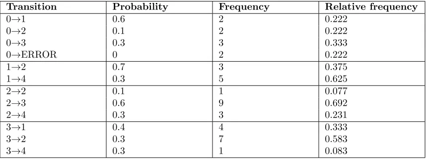
Transition Probability Frequency Relative frequency

0→1 0.6 2 0.222

0→2 0.1 2 0.222

0→3 0.3 3 0.333

0→ERROR 0 2 0.222

1→2 0.7 3 0.375

1→4 0.3 5 0.625

2→2 0.1 1 0.077

2→3 0.6 9 0.692

2→4 0.3 3 0.231

3→1 0.4 4 0.333

3→2 0.3 7 0.583

3→4 0.3 1 0.083

Table 3: Relative frequencies after nine tests, including failures

Note that we are discussing trend analysis here, not a single value.

3.3

Reliability

Once the discriminant is sufficiently close to zero, we can compute the reliability R. This value can be interpreted as an estimate of the single use reliability: the probability that a random single test (from the initial to the final state) can be executed without the occurrence of failures. So, if the value of R is 0.976, we can say that a randomly selected test sequence has 97.6% chance to execute successfully without failure.

The value for R is computed according to equation 3. Note that it is not necessary to achieve complete transition coverage in order to compute the reliability, but that the resulting reliability value should only be used once the discriminant approaches zero.

Rinit,f inal= ˆpinit,f inal+ Σj∈t(ˆpinit,j∗Rj,f inal) (3)

Here init is the initial state, final is one of the final states, and t is the set of transient (non-absorbing) states. The formula assumes that there is only one final state. If this is not the case, the reliability can be found by summing the reliabilities from the initial state to each of the final states. Alternatively, the model can easily be converted into one with a single final state, by introducing a new state that will be the final state, and by including transitions from all original final states to this state. These transitions will have probability one. Then, we can make the original final states regular states, which results in a equivalent system with a single final state.

In order to clarify this formula, we will apply it to a small example. This example will be very similar to the one used in explaining the discriminant computation, but here we will introduce some failures. Let’s assume that the transition from state 0 to state 1 is faulty, and that it has failed twice. The resulting relative frequencies are summarized in table 3.

.

states t contains states 0, 1, 2, and 3. States 4, and ERROR are not included. The probabilities ˆ

pi,j can be found in Table 3. If there is no entry, the probability is equal to 0, and the term can be

dropped from the formula. Entering the probabilities into the formula yields the following equation (equation 4):

R0,4= 0 + (ˆp0,0∗R0,4+ ˆp0,1∗R1,4+ ˆp0,2∗R2,4+ ˆp0,3∗R3,4)

= 0 + 0∗R0,4+ 0.222∗R1,4+ 0.222∗R2,4+ 0.333∗R3,4

= 0.222∗R1,4+ 0.222∗R2,4+ 0.333∗R3,4

(4)

Similarly, we can determine the equations forR1,4,R2,4, andR3,4. The resulting system of equations

can be found below (equation 5)

        

R0,4= 0.222∗R1,4+ 0.222∗R2,4+ 0.333∗R3,4 R1,4= 0.625 + 0.375∗R2,4

R2,4= 0.231 + 0.077∗R2,4+ 0.692∗R3,4 R3,4= 0.083 + 0.333∗R1,4+ 0.583∗R2,4

(5)

All that remains is solving a system of linear equations. The solution to the system in equation 5 is shown in equation 6. The single use reliability, which is the probability that a single test run from the initial state 0 to the final state 4 executes without any failures, is estimated byR0,4, which is

approximately equal to 0.776. This means that any random test case has a 0.776 probability of executing without failures.

Note that we use the approximation sign in the formulae in equation 6. This is due to the fact that we work with numbers that were rounded up or down, in order to make everything more readable. Also note that the computation of R places complete faith in the test history. If no failures have occurred, the reliability will be one (as it is in states 1, 2, and 3 in our example).

        

R0,4≈0.776 R1,4≈1 R2,4≈1 R3,4≈1

(6)

3.4

Mean time between failures

Finally, [22] introduces the mean time between failures. This is the expected amount of transitions between the occurrences of two failures. In order to compute M, we need to slightly adjust the model we are working with by introducing a transition from all terminal states (terminal error states, and terminal final states) to the initial state. This is due to the fact that the computation contains a steady state computation. Equation 7 shows the formula for computing the mean time between failures.

where vi is the conditional long-run probability for failure state i: given that the process is in a

failure state, what is the probability that it is in state i?,mj is the mean number of steps until the

first occurrence of any failure state from usage state j, u is the set of usage states, f is the set of failure states.

We will apply this formula to the same example as above: the one where the transition from state 0 to state 1 has caused a failure twice. The absolute and relative frequencies are summarized in table 3. We can use the relative frequencies from this table as probabilities ˆpi,j, but before we

can compute the mean time between failures, we first need to know the values forvi andmj.

As mentioned above, vi is the conditional long run probability for a failure state i, given that

the process is in a failure state. Basically this means: if we know that we’re in a failure state, what is the probability that it is failure state i. To find this number, we need to compute the steady state distribution of the testing chain T. The steady state probability that the system is in a failure state is the sum of the steady state probabilities of all failure states. Vifor any state can be computed by

dividing the steady state probability for that state by the steady state probability that the system is in a failure state (vi =Pπi

s∈fπs).

Since we only have one error state,vi =ππii = 1.

Mj is the mean number of steps until the first occurrence of any failure state from usage state

j. This can be computed by the following formula (equation 8). In this formula, usage state j should be substituted for p, and q is one of the error states.

mpq= 1 +

X

r6=q

ˆ

ppr∗mrq (8)

By simply entering the relative frequencies (and 0 whenever there is no entry in the table for a specific transition), we obtain the following set of linear equations (equation 9). These solutions can be solved, which results in the values shown in equation 10. The computation of mean time between failures M is summarized in table 4.

                  

m0= 1 + (0.222∗m1+ 0.222∗m2+ 0.333∗m3+ 0.222∗mERROR)

m1= 1 + (0.375∗m2+ 0.625∗m4)

m2= 1 + (0.077∗m2+ 0.692∗m3+ 0.231∗m4) m3= 1 + (0.333∗m1+ 0.583∗m2+ 0.083∗m4)

m4= 1 + (1∗m0)

mERROR= 0

(9)                   

m0= 21.600

m1= 25.251

m2= 27.002

m3= 27.027

m4= 22.600

mERROR= 0

(10)

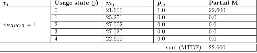
vi Usage state (j) mj pˆij Partial M

vERROR= 1

0 21.600 1.0 22.600

1 25.251 0.0 0.0

2 27.002 0.0 0.0

3 27.027 0.0 0.0

4 22.600 0.0 0.0

sum (MTBF) 22.600 Table 4: Computation of mean time between failures after nine tests in example 1

observations are, firstly, that the mean time between failures for our example is not completely correct, due to the fact that we’ve slightly changed the model. This means that the transitions we’ve added between the final state and the initial state are also counted as a step between the failures. Per successful test, one reset transition is included in M. To counter this, we would have to estimate the average test length, and subtract those additional steps from the total. Additionally, the formula also counts the transition that fails as a step. Thus, the minimum of M is 2.

Finally, note that we are only dealing with terminal failures, i.e. failures that force the system to terminate. It is also possible to encounter non-terminal failures. In this case, there will be outgoing transitions from error states to usage states. In our tool, we only deal with terminal failures, but this is an interesting area for future work.

4

Post processer tool

This section is focused on the on-the-fly post processing tool that was developed. We will explain its purpose in section 4.1, and give some usage instructions in section 4.2. Section 4.3 shows the tool’s structure, and section 4.4 shows how it could be extended with different input languages, or reliability measures.

4.1

Purpose

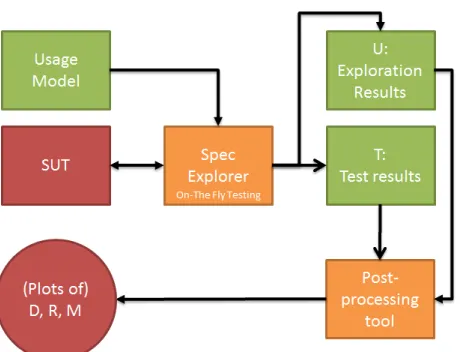
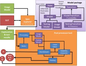
The idea behind this tool is to use Spec Explorer’s OTF output as the basis for some calculations. When you perform on-the-fly tests on your system, the results are stored in the form of Spec Explorer exploration files (.seexpl). This record of the tests performed can be used to say something about the reliability according to several measures that were mentioned above: discriminant, reliability, and mean time between failures. This cooperation is shown in figure 5.

In principle, the reliability measures that were selected are used in statistical testing: testing based on a usage model. However, a regular model has an implicit usage model: the uniform distribution. This means that each outgoing transition from a given node is chosen with the same probability.

Figure 5: Integration of Spec Explorer and our post processor tool

4.2

Using the tool

4.2.1 Important model properties

There are a few important properties a model must have, in order to make sure that the tool will work correctly.

• The model must have exactly one initial state.

• A probe must be defined. It must be used to ensure that all states have a unique name.

• State names cannot start with ”ERROR ”. This is a prefix reserved for error states.

• At this point in tool development, non-determinism is not allowed.

4.2.2 Introducing probabilities into the model

As we mentioned above, a regular model already has an implicit usage profile. Thus, when no usage model is provided, the tool will assume a uniform distribution. However, it also provides a way for the user to specify a different usage model.

We use Spec Explorer’s requirements structure to incorporate our probability information into the model, and the tests generated from it. In the model file, you can use the requirement capture method to attach a requirement to a transition. For example:

[ R u l e ( A c t i o n = " O p e n () / r e s u l t ") ] s t a t i c int O p e n ()

{

C o n d i t i o n . I s T r u e ( s t a t e == S t a t e . C l o s e d ) ; s t a t e = S t a t e . O p e n e d ;

r e t u r n 0; }

In the example above, the probability of taking transition ”Open” from state ”Closed” is set to 0.8. In order for the tool to be able to extract this probability, the notation is crucial: it has to be a lowercase p, followed by a space, an equals sign and another space. After this, the probability needs to be specified as a double between 0 and 1. Additionally, the probabilities can only be added to active transitions: transitions that provide an input to the system under test (as opposed to actions that report on outputs from the system under test). And finally, a correct usage model should be provided, where for each state, the probabilities on the outgoing transitions sum to 1.

At this moment we have not yet adapted the online test generation algorithm in Spec Explorer. Therefore, we cannot yet say anything useful on the reliability of models with a specified usage model.

4.2.3 Using the tool

The tool works with Spec Explorer’s on-the-fly test results. This means that the user will need to provide the location in which these test results can be found. Additionally, the tool needs to know what the original model looks like. Therefore, it also needs the location of the model.

There are several possible outputs that can be provided: relative frequencies, the discriminant, the mean time between failures, the reliability, and the development of these last three measures over time, all described in section 3. The tool allows for both separate and simultaneous computation of these measures. The user can specify their preference by setting an option.

To use the tool, open up a command prompt window and go to the directory that contains the .exe file. For example:

> cd " U s e r s \ j e n n y . den . o u d e n \ D o c u m e n t s \ V i s u a l S t u d i o 2 0 1 0 \ P r o j e c t s \ P o s t p r o c e s s i n g OTF run \ P o s t p r o c e s s i n g OTF run \ bin \ D e b u g "

Call the tool with the following arguments: path to the exploration file of the model, path to the folder containing the OTF test results, and option. The possible options are -r for relative fre-quencies, -d for discriminant, -p for plotting the discriminant over time, -w for Whittaker reliability, -pr for plotting the reliability over time, -wm for Whittaker mean time between failures, -pm for plotting the mean time between failures over time, and -all for all of the above. The default option enables all whittaker options, (d, p, w, pr, wm, pm). For example:

> " P o s t p r o c e s s i n g OTF run . exe " " C :\ U s e r s \ j e n n y . den . o u d e n \ D o c u m e n t s \ V i s u a l S t u d i o 2 0 1 0 \ P r o j e c t s \ V o o r b e e l d V e r s l a g \ E x p l o r a t i o n R e s u l t s \ A c c u m u l a t o r M o d e l P r o g r a m . s e e x p l " " C :\ U s e r s \ j e n n y . den . o u d e n \ V i s u a l S t u d i o 2 0 1 0 \ P r o j e c t s \ V o o r b e e l d V e r s l a g \ V o o r b e e l d V e r s l a g \ T e s t R e s u l t s \ A c c u m u l a t o r M o d e l P r o g r a m \2016 -01 -04 14 _ 3 6 _ 3 9 " - all

4.3

Tool structure

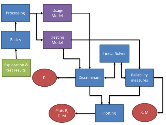
Figure 6: Structure of post-processing tool

The green rectangle represents an input to the system: the exploration and test results, U and T, which are the Spec Explorer exploration of a model, and the Spec Explorer test results obtained from that model respectively. They are inputs to the basics module. The red ellipses represent outputs. They are numeral values D, R, and M, which represent the discriminant, reliability, and mean time between failures; as well as plots for each of these three measures.

Blue rectangles represent modules. A module represents a single component or functionality in the system. It can take inputs, from other modules or from the user, and it can provide outputs, to other modules or to the user. The tool contains a total of six modules. We will provide a short description of each of them.

The first module is Basics. The purpose of this module is to collect the user input, and pass it on to the relevant modules. It makes sure that the exploration file is processed, and that each individual test set is considered. Additionally, if the user has provided a parameter, the Basics module makes sure that only the computations that were specified by the user are carried out.

Next, we have the Processing module. This module gets individual exploration files. If the input is the exploration of the Spec Explorer model, the Processing module uses it to construct the usage chain. If the input is a test case, the Processing module adds it to the testing chain.

The Discriminant module uses the usage model and testing model that were constructed by the Processing module to compute the discriminant. It also needs the linear solver, to find the steady state distribution of the usage model. If the user only wants the discriminant value for the entire test set, the Discriminant module is applied after all test cases have been processed, and the testing model is complete. If the user wants a plot of the discriminant over time, the module is used each time a test case is added to the testing model. The results are stored, and once the testing model is completed, they are displayed in a graph.

Similarly, the Reliability measures module uses the testing model to compute either the reli-ability, or the mean time between failures. The computation of the reliability consists of solving several linear equations, which is why it needs to use the Linear Solver module. Computation of the mean time between failures also relies on the Linear Solver. First of all, the computation requires the conditional steady state distribution, for which we need the Linear Solver. Second of all, the computation relies on mj, which is the mean number of steps until the first occurrence of

any failure, starting from state j. Thismj is also computed by solving a system of linear equations

with the Linear Solver. Like the discriminant, reliability and mean time between failures can both be computed over the complete test set, and plotted over time.

The final module is the Plotting module. This module gets two sets of values, and plots them against each other. The first set of values contains the test numbers. These are included, because the discriminant and mean time between failures cannot be computed at all times. The second set of values are the discriminant, reliability, or mean time between failures values for the testing model constructed up to and including the test with that test number. As well as plotting the graphs, the Plotting module also stores a copy of the graph, and a csv file containing both datasets in the map with Spec Explorer test results.

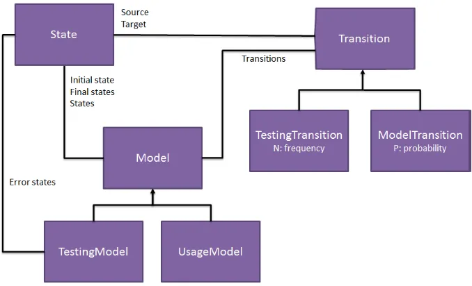
Finally, the purple rectangles represent global variables of the type Model; a type which we have introduced ourselves. This type is used to store the Usage Model and Testing Model as displayed in figure 6. Figure 7 shows the structure of the Model package. Basically, a model consists of three main parts: Model, State, and Transition. Model is the overview class, from which the entire model can be accessed. A model has an initial state, a set of final states, a set of all states, and a set of all transitions.

Model has two subclasses: TestingModel and UsageModel. UsageModel is used to store the usage model, which is extracted from the exploration of the Spec Explorer model. TestingModel is used to store the testing model, which is extracted from the test set. Since the testing model can contain failures, we add a set of error states to TestingModel, to keep track of them.

The transitions can also be one of two subclasses: TestingTransition, and ModelTransition. The difference between these two is that a TestingTransition has a frequency, whilst a ModelTransition has a probability. Every transition has a source and a target state.

There is only one State class, but there are different types of states: error states, initial states, accepting states, and regular states. The type of a class can be specified in the constructor. We chose not to use inheritance in this case, because it is possible for a state to be both initial and accepting.

Figure 7: Model Package

rectangles are classes. The purple rectangles in the post-processor tool are objects of the types Us-ageModel and TestingModel. These classes, along with the other modelling classes, are contained in the Model package, shown as a light purple rectangle.

4.4

Extendability

It’s possible to extend the tool to work with another input language. For this, one has to provide their own version of the Basics and Processing modules, in order to translate their model and tests into a usage model and testing model respectively.

Note that the basics module is also responsible for extracting the options supplied by a user, and calling the respective computation methods, as well as storing intermediate results for plotting.

Additionally, it is possible to add extra, or different reliability measures to the tool. This can be done by introducing a new module similar to Discriminant and Reliability measures. This mod-ule should be able to work based on the usage and testing models, and it should be called from the Basics module. This means that not all measures will be suitable to extend the tool.

In this section we will carry out several experiments with the tool, to see the practical difference between the values and respective development over time of the discriminant, the reliability, and the mean time between failures.

We have constructed two example models, and thus, we have divided our experiments into two rounds. Each of these rounds will be elaborated upon below.

5.1

Simple example model

The model for the first round of tests is a very simple model without meaning. It is equivalent to the model in example 1 (figure 1). State 0 corresponds to Start, state 1 corresponds to Left, state 2 corresponds to Middle, state 3 corresponds to Right, and state END corresponds to End.

There is an initial state, from which one of the actions Left(), Straight(), and Right() can be chosen. This leads to one of three states Left, Right, and Middle, between which the system can move using the same actions. Additionally, from these three states, the system can enter the final state End by taking action End(). The final state is absorbing, so a test case is complete once the final state is reached.

Figures 9 and 10 show the example model with two different distributions: a usage distribution, and a uniform distribution, modeled in Spec Explorer. The initial state is gray, the final state has a green border, and the text on the transitions describes the action and the return value expected from the system, as well as the transition’s probability. For example, the transition from state Start to state Right in the usage model has the following text: Right()/0, Captured: p = 0.3. This means that this transition is taken when the action Right() is chosen from state Start. We expect the return value 0, and when any other value occurs, the test fails. According to the usage model, this transition is taken with probability 0.3. The output is specified because Spec Explorer uses it as a means to detect failures. If the model’s output and the test’s output do not match, a failure is recorded. When the expected output is unspecified, the associated action does not have a return value.

The above model was used to generate on-the-fly tests in a dummy implementation that we sup-plied. This implementation did nothing, except return a value when a method was called. If that value matched the one in the model, the transition would be crossed successfully. If the values in the model and in the implementation did not match, a failure occurred, and the test terminated.

In between tests, the implementation was adjusted manually, in order to introduce failures and create diverse test sets. The resulting set of test sets that was carried out is summarized in table 5, along with the values for the discriminant, reliability, and mean time between failures that were computed over each set. If possible, the progress over time of each measure was graphed. In the interest of readability, these graphs were combined into several plots, which are included in figure 11, and figure 12.

The table shows how many tests were performed in each test set, as well as how many failures occurred. The failures were introduced in a dummy implementation that could return incorrect return values. The column ”Remarks” shows the nature of the failures that were introduced.

Figure 9: Spec Explorer usage model of example 1

(a) Discriminant over time for test sets 1.1, 1.2, 1.6, and 1.9

(b) Discriminant over time for test sets 1.3, 1.7, 1.11, and 1.14

(c) Discriminant over time for test sets 1.8, 1.10, 1.15, and 1.16

(a) Reliability over time for test sets 1.1, 1.2, 1.3, and 1.4

(b) Reliability over time for test sets 1.5, 1.6, 1.7, and 1.8

(c) MTBF over time for test sets 1.1, 1.2, 1.3, 1.4, 1.5,

1.6, and 1.7 (d) MTBF over time for test set 1.8

Test set Nr of tests Nr of failures Remarks Type of model

D R M

1 354 0

Usage 0.1525 1 -1

Uniform 0.0017 1 -1

2 346 100 Half the actions

”Straight” fail

Usage 0.1896 0.7118 13.44 Uniform 0.1997 0.7118 13.44

3 354 101

New random seed, setup test set 2

Usage 0.2385 0.7127 13.32 Uniform 0.2009 0.7127 13.32

4 353 353 All actions

”End” fail

Usage -1 0 4.78

Uniform -1 0 4.78

5 354 354 All transitions

fail

Usage -1 0 2

Uniform -1 0 2

6 350 24 One step in 50

fails

Usage 0.1825 0.9315 67.29 Uniform 0.0257 0.9315 67.29

7 352 24 24 steps in a

row fail (13-36)

Usage 0.1726 0.9320 67.57 Uniform 0.0237 0.9320 67.57

8 355 24 24 steps fail in a row (267-290)

Usage 0.1739 0.9326 67.99 Uniform 0.0236 0.9326 67.99

Table 5: Summary of first round of experiments

Note that this is only the case because we are using the same test results. When Spec Explorer can generate tests based on a usage model, a different test set would be generated, and the values would not be the same.

5.2

Simplified case study

The second round of tests is based on a different, and slightly bigger model. This model is based on a large car reservation system that was co-developed by Nspyre. Due to confidentiality issues, our model is a simplification of adding a new car to the system.

Even this simplified model is too large to display as an image in this report. We have therefore included a very abstract representation of our model in figure 13.

State Transition Usage Probability Uniform probabil-ity

ReservationForm [Null, Null]

addCar 1 1

ConfirmationForm [Ford, Eindhoven]

close 1 1

ConfirmationForm [Renault, Eindhoven]

close 1 1

AddCarForm[X, Y], where X==0 OR Y!= Eindhoven

addModel(Renault) 0.30 1/6

addModel(Ford) 0.15 1/6

addStation(Eindhoven) 0.30 1/6 addStation(Utrecht) 0.15 1/6

addClass 0.05 1/6

cancel 0.05 1/6

AddCarForm[X, Y], where X!=0 AND Y== Eindhoven

addModel(Renault) 0.20 1/7

addModel(Ford) 0.10 1/7

addStation(Eindhoven) 0.20 1/7 addStation(Utrecht) 0.10 1/7

addClass 0.05 1/7

cancel 0.05 1/7

confirm 0.30 1/7

Table 6: Summary of probabilities in car reservation model

by selecting the option ”add car”, the system moves to a new stage. This represents the form for adding cars. In this stage, the user can cancel and move back to the first stage, or they can add one of three types of information to the form: a car class, a car type, and a car location. The latter two are mandatory options. To prevent a state space explosion, we’ve limited the car types to either Renault, or Ford, and we’ve limited the locations to Eindhoven, or Utrecht. The class is an empty method; it’s just there to show that adding a class is an option, but we haven’t specified any possible inputs.

Once all mandatory options are supplied, the user can move on to the confirm form. However, there is a guard on this transition: the location must be Eindhoven, and the type of the car must have been specified. If the guard is satisfied, the system moves to the third stage: the confirmation stage. In order to represent this, we have used two add car form stages. In the first, the guard condition is not satisfied, in the second, it is. The system can move between these two according to its current state. We use this representation in order to be able to show the transition probabilities we have assigned. The purple probabilities are those that occur when a uniform distribution would be used. The orange ones are those that occur when the usage model is used.

From the add car form stage, the user can move back to the idle stage by closing the confirmation form.

Like in the previous round of experiments, there are two versions of the model: one with a usage distribution, and one with a uniform distribution. These are shown in table 6.

Test set Nr of tests Nr of failures Remarks Type of model

D R M

1 350 0

Usage 0.2204 1 -1

Uniform 0.0062 1 -1

2 350 350 all steps fail

Usage -1 0 2

Uniform -1 0 2

3 350 71 failure distance

is 50

Usage 0.2625 0.8795 50.39 Uniform 0.0389 0.8795 50.39

4 350 71 failure distance

0, offset 100

Usage 0.2632 0.8795 49.45 Uniform 0.0384 0.8795 49.45

5 350 71 failure distance

0, offset 3000

Usage 0.2430 0.8795 49.80 Uniform 0.0386 0.8795 49.80

6 350 1 offset 500

Usage 0.2207 0.9985 4375 Uniform 0.0065 0.9985 4375

7 350 36

generated with failure

probability 0.01

Usage 0.2370 0.9426 109.28 Uniform 0.0219 0.9426 109.28

8 350 209

generated with failure

probability 0.1

Usage 0.3736 0.5466 10.70 Uniform 0.1894 0.5466 10.70

Table 7: Summary of second round of experiments

that value matches the one predicted by the model, the transition succeeds, otherwise, a failure is recorded and the test fails. The dummy implementation was adapted in between each test set, in order to introduce failures in different places.

The resulting test sets that were carried out are summarized in table 7. This table also contains the values for the discriminant, reliability, and mean time between failures. The graphs were combined into multiple plots for readability. They are shown in figure 14 and figure 15.

(a) Discriminant over time for test sets 2.1, 2.3, 2.4, 2.7, and 2.14

(b) Discriminant over time for test sets 2.5, 2.9, 2.11, 2.12, and 2.15

(c) Discriminant over time for test sets 2.6, 2.8, 2.13, and 2.16

Figure 14: Discriminant over time

probabilistically.

(a) Reliability over time for test sets 2.1, 2.5, 2.6, and 2.7

(b) Reliability over time for test sets 2.2, 2.3, 2.4, and 2.8

(c) MTBF over time for test sets 2.2, 2.3, 2.4, 2.7, and

2.8 (d) MTBF over time for test set 2.5, and 2.6

6

Discussion

In this section, we will look at the results that were obtained in the experiments in section 5. We will repeat the purpose of each of the three measures, and study the influence of the failures that were introduced in the experiments. Additionally, we will point out some limitations of the tool, as well as some possible future enhancements.

6.1

Discriminant

The discriminant was introduced as a measure of similarity between the usage chain and the test-ing chain. The premise is that if the models are similar enough, transitions to error states are negligible, and the testing chain is suitable for use in computing the reliability and mean time be-tween failures of the system. When the two models are exactly the same, the discriminant will be 0.

Computation

In order to compute the discriminant, each transition in the usage model must be crossed at least once in the testing model. This is evident from equation 1, which contains the fraction pij

ˆ

pij. If ˆpij

is 0, this fraction and the discriminant are undefined.

We can see this in our experiments in two ways. Firstly, none of the discriminant over time plots start for x equal to 0. Take the plot in figure 16 for example. The test set in this experiment is one where each transition fails with a probability of 0.01. The first point at which the discriminant can be computed is after approximately 30 tests.

Secondly, for some test sets, the discriminant can never be computed. This occurs when one or more of the transitions in the usage model remain uncrossed in the testing model. Test sets 1.4, 1.5, and 2.2 show this issue. In test set 1.4. all tests fail because the End() action always fails. This means that the testing model will contain a transition from states Left, Middle, and Right to an error state, which is taken with probability 1. The correct transitions to state End have probability 0, because they are never crossed, and thus, the discriminant can never be computed.

Test sets 1.5, and 2.2 are sets in which each transition fails. This means that all transitions in the testing model with a frequency that is higher than 0 are error transitions. None of the correct transitions are ever crossed, and the discriminant cannot be computed. Figures 11 and 14 do not

Figure 17: Discriminant over time for test set 2.5b (Uniform - failure distance 0, offset 3000)

contain a plot of the discriminant for any of these test sets (1.4, 1.5, 2.2).

Effect of failures

Since the discriminant measures similarity, and the usage model doesn’t contain any failures, we expect the value of the discriminant to increase when errors occur. This is supported by test set 2.5 (figure 17). In this test set, 71 consecutive failures are introduced around the 250th test case. The graph clearly shows an increase at that point.

As a result, we expect that the discriminant will only approach 0 when relatively few failures occur. The discriminant values in table 7 support this idea. Specifically, when looking at the values for test sets with a uniform distribution, it clearly shows that the discriminant value is higher, the more failures occur in a test set. For test set 2.1, which contains no failures, and test set 2.6, which contains one failure, the discriminant after 350 tests is smaller than 0.01.

Moreover, we expect that the effect of failures near the start of testing is larger than the effect of failures near the end of testing. This is due to the fact that when there are fewer transitions, one failure transition has a higher relative frequency than when there are many transitions. In the long run, each equivalent failure will have the same effect on the discriminant.

This expectation is confirmed by test sets 1.7 and 1.8. In test set 1.7, 24 consecutive failures occur near the start of testing. Its development over time is shown in figure 18 In test set 1.8, 24 consecutive failures occur near the end of testing. The discriminant over time for this test set is shown in figure 19.

In figure 18, we see the discriminant jump from approximately 0.12 to approximately 0.45: a difference of about 0.33. The difference in figure 19 is only about 0.025. However, we also see that the discriminant values after 350 tests are almost equal for both test sets: 0.0237 and 0.0236 respectively (see table 5). This shows that the eventual value of the discriminant is similar, even though the time of occurrence of the failures, and their effects on the discriminant at the time of occurrence, are different.

Miscellaneous observations

Figure 18: Discriminant over time for test set 1.7b (Uniform - 24 steps in a row failed)

Figure 20: Discriminant over time for test set 1.8a (Usage - 24 steps in a row failed later in the test)

distribution, and when there are few failures. In Spec Explorer, tests are generated probabilisti-cally with a uniform distribution. Thus, in our experiments, the discriminant should only approach zero when we test a uniform model. This is supported by the experiment outcomes in tables 5 and 7.

Second of all, we want to remark that the discriminant is not a monotonous function: it is possible for the discriminant to go up, when failures occur, or when statistically unlikely paths are taken. The fact that the discriminant can increase means that simply reaching a certain threshold value isn’t necessarily a good enough stopping or reliability criterion. Instead, the discriminant should be allowed to stabilize (which happens by carrying out a large amount of tests), or decisions should be based on trends in the development of the discriminant over time.

Unfortunately, [22] doesn’t provide any hand holds on this. If we want to use the discriminant as a stopping criterion, we will need to look into this.

Finally, some of the plots of the discriminant over time seem to follow an upward trend, whereas we expect a downward one. An example is the plot for test set 1.8b, shown in figure 20. Test set 1.8 contains 24 consecutive failures around test 250. However, even disregarding these failures in the graph, there is an upward trend. We assume that this happens because the test set is based on the usage model. Since Spec Explorer generates tests according to the uniform model, the discriminant will never approach zero on the long run. However, before stabilization the testing model might coincidentally resemble the usage model, resulting in a smaller discriminant.

This assumption is strengthened by the fact that none of the test sets based on the uniform model have an upward trend in the development of their discriminant over time.

6.2

Reliability

Figure 21: Whittaker reliability over time for test set 2.5 (failure distance 0, offset 3000)

Computation

There are no restrictions on the computation of the reliability. As soon as the first test is completed, the reliability can be computed. However, the resulting value is only meaningful if the discriminant approaches zero. This can be shown in two examples.

First of all, there could be too few tests. For instance, consider test case 2.5. This test case contains 71 consecutive failures from about test 250 onwards. Figure 17 shows that the discriminant is defined from 30 tests onward. Before this point, not even all transitions are crossed. Nonetheless, the reliability, shown in figure 21 is 1. According to the computation, the probability of successfully executing any single test case is 100 %, even when there are some transitions that have never been tested.

Second of all, the incorrect usage distribution could influence the weight of a failure. Let us illustrate this with a small example: a system with a single state, and two self loops. In the usage model, loop a is taken with a probability of 0.9, and loop b is taken with probability 0.1. Now, we assume that loop b always fails. Intuitively, we would expect the single use reliability of this system to be 0.9: 0.9 from a, which always succeeds, and 0 from b, which always fails.

Next we assume that the actual distribution in the testing model is a uniform distribution. This means that the discriminant would not be approaching zero. When the reliability is computed based on this distribution, it would be 0.5: 0.5 from a, which always succeeds, and 0 from b, which always fails.

Effect of failures

We expect the reliability of a system to drop when failures occur, and to converge to one when cor-rect tests are carried out. Our experiment results support this. For instance, test set 2.6 illustrates this very clearly. This test set contains one failure. The reliability plot for this test set is shown in figure 22. The reliability for this test set is 1, until it shows a drop around test 35, where the single error occurs. From that point on, all tests succeed, and the reliability grows towards 1.

Following from this, we expect the reliability to be lower if the testing model contains more failures, and vice versa. This is supported by the reliability values in tables 5 and 7.

Figure 22: Whittaker reliability over time for test set 2.6 (1 failed)

same. This is confirmed by test sets 1.7 and 1.8. Both these test sets contain the same amount of failures, but the failures in test set 1.7 occur early on in the testing process, whereas the failures in test set 1.8 don’t occur until the 250th test. Nevertheless, the reliability for both these test sets is nearly the same.

Unfortunately, we cannot yet alter the testing distribution. However, once the desired adapta-tions to Spec Explorer have been made, some experiments should be dedicated to studying the influence of different testing distributions on the reliability.

Miscellaneous observations

There are two more issues that we would like to discuss. First of all, we want to emphasize that the computation of the reliability is completely based on the test results. This means that the reliability is 1 if all tests succeed, it is 0 if all tests fail, and otherwise it is somewhere in between. However, how realistic is it to say that the reliability of your system is 1 if no failures have occurred thus far? Even when the discriminant is equal to zero, and no failures have occurred, one still might occur in the future.

The only way to solve this issue is to look into different reliability measures, such as LeGuen [6], and Sayre [11].

Second of all, the reliability for test sets 2.3, 2.4, and 2.5 are exactly the same. Each of these test sets consists of 350 tests, and 71 failures, but the places in which those failures occur are different. In test set 2.3, one failure occurs every 50 transitions. In test set 2.4, all 71 failures occur consecutively, and they occur near the beginning of testing. In test set 2.5, the failures also occur consecutively, but they take place near the end of testing.

Looking into this, we discovered that the reliability could be computed as 1−N umber of f ailures N umber of tests

for both our experimental setups. However, this is not apparent from the data in result tables 5 and 7. For the first round of experiments, this is due to the fact that we stopped the on-the-fly testing manually. This means that the test that was in progress was immediately aborted when the stop button was pressed. As a result, the test sets in the first round of experiments might contain an additional partial test, causing slight deviations from the value computed with our formula.

the values provided by the tool, either. The reason for this is the structure of the model. Unlike the model in the first round of experiments, this model doesn’t have an absorbing final state: it’s possible to continue testing once the final state is reached. The tool’s reliability estimation depends on a model with an absorbing final state, so we simulate this by splitting each test into subtests consisting of single runs that end as soon as the test returns to the final state. Since the final state is also the initial state, we can see how many simulated tests were run by counting the number of outgoing transitions from the initial state. Using this number as the amount of tests, we get the exact values we expected from our formula.

This also explains why we found three values that were exactly the same for test sets 2.3, 2.4, and 2.5: each of these test sets contained 71 failures, and there were 589 outgoing transitions from the initial state. The fact that each of these three test sets has the same amount of simulated tests could be a coincidence. It could also be due to Spec Explorer’s settings, but it has nothing to do with the computations carried out by our tool.

At this point in our research, we are not able to explain why the tool’s reliability values match those computed with the formula introduced in this paragraph. We have studied the computations and examples in detail, but the solution is not yet evident. Due to time constraints, we need to leave this issue unsolved. We hope that future research will look into it.

6.3

Mean time between failures

The mean time between failures is the expected number of transitions between two failures. This value, too, is computed solely based on the testing model, so the results within a test set are the same. When all transitions fail, the mean time between failures will be 2: the failing transition, and the implicit transition back to the initial state. The fewer transitions fail, the higher the mean time between failures.

Computation

The mean time between failures can be computed as soon as at least one failure has occurred. Here, too, the resulting value is only meaningful if the discriminant approaches zero.

The computability is supported by test sets 1.1 and 2.1. Both these test sets do not contain any failures, and we can see in tables 5 and 7 respectively that the mean time between failures for these test sets is not defined (-1). Additionally, consider test set 2.6. This test set contains a single failure, so what we expect to see is that the mean time between failures is undefined until this failure occurs, after which it keeps growing. The plot included in figure 23 confirms this.

To show the importance of the discriminant approaching zero, we will employ the same exam-ple as for reliability: a system with one state and two self loops a, and b. According to the usage model, a is selected with probability 0.9, and b with probability 0.1. If loop b always fails, we expect the mean time between failures to be 10: for every time transition b is selected, transition a will be selected 9 times, which means a total of 10 steps.

However, when the testing distribution is uniform, and the discriminant doesn’t approach zero, the mean time between failures will be 2: for every time transition b is selected, a is selected once, which means a total of two steps.

Effect of failures

exe-Figure 23: Mean time between failures over time for test set 2.6 (1 failed)

Figure 24: Mean time between failures over time for test set 1.6 (1 step in 50 failed)

cuted, we expect it to rise. The plot of the mean time between failures over time for test set 1.6 confirms this. Test set 1.6 contains one failure every 50 steps. In the graph in figure 24, we clearly see that the mean time between failures keeps growing. Every 50 steps (approximately 10 tests) we see a sharp drop in the mean time between failures. This is where the failures occur.

As a result of this first observation, we expect the mean time between failures to be higher, the fewer failures are found in the test set. Conversely, when the test set contains very many fail-ures, we expect the mean time between failures to be low. This is supported by the MTBF values in tables 5 and 7.

Thirdly, as with the discriminant and reliability, the effects of failures that occur near the start of the test set are different from the effects of later failures. In principle, failures near the start of the test set will have a larger influence on the mean time between failures than failures near the end of the test set. The graph in figure 24 shows this: the first peaks are significantly higher than the last ones.

Figure 25: Mean time between failures over time for test set 1.7 (24 steps in a row failed)

Figure 26: Mean time between failures over time for test set 1.8 (24 steps in a row failed later in the test)

set 1.7 occur near the start of the test set, and the failures in 1.8 occur near the end, but figure 25, which shows the MTBF for test set 1.7, shows a peak that is significantly lower than the one in figure 26, which shows the MTBF for test set 1.8.

This phenomenon makes sense, though. Since both test sets contain the same amount of failures, and the same amount of tests, we expect the eventual values of the MTBF to be fairly close to each other. Table 5 shows that this is indeed the case. In test set 1.7, the first failure occurs in test 13. This means that there were 12 tests worth of correct transitions to balance out this first failure. In test set 1.8, the first failure doesn’t occur until test 267, which means there are 266 tests worth of correct transitions to balance out this first failure, resulting in a significantly higher peak.

Miscellaneous observations