Navigation for PDT in the paranasal sinuses using virtual views

(1)

Navigation for PDT in the paranasal sinuses

using virtual views

L.E. (Laura) Visser

MSc Report

Committee:

Dr.ir. F. van der Heijden Dr. F.J. Siepel Ir. E. Molenkamp R.L.P. van Veen, PhD

Dr. M.B. Karakullukcu

May 2019

014RAM2019 Robotics and Mechatronics

EE-Math-CS University of Twente

(2)

1 Introduction

Cancer in the paranasal sinuses is a serious disease. Successful surgical or radiation treatment in which the tumor will not recur is a challenge. Not only is a wide variety of tumors covered by the description sinus malignancies, each with their own biological characteristics and prognosis[1], but these tumors are also growing in regions where critical structures are very nearby. Because of the presence of these delicate structures, like the orbit, carotid arteries and the skull base, in many cases the margins that can be achieved with surgery and radiation therapy are not sufficient. Incomplete removal increases the chance for the tumor to recur. Due to these difficulties the recurrence-free survival rate after five years is less than 50% [2].

Figure 1: The different paranasal sinuses [3]

Photo Dynamic Therapy (PDT) is a relatively new and lesser-known method, which can extend the margins after surgery and thereby potentially decreases the chance of recurrence. In this treatment, a photosensitizing agent which is localized in the tumor, is activated by a light source. A cytotoxic process occurs resulting in cell death[1], [4]. It can be used to increase the margins after surgery by 5-10mm, thereby destroying the leftovers of the tumor[5]. Radiation is not desirable to repeat in this area, since it poses a high risk for complications, in particular for damage to the optical structures[6]. PDT however, is repeatable, and does not compromise other treatments as radiation or chemotherapy[7].

Without a 3D view of the surgical scene, as is the situation in current endoscopic procedures, the task of navigation is difficult[8], [9]. In order to avoid the critical structures and to enable placing the light source at the most effective location, precise navigation is necessary, and good orientation of the surgeon in the complex cavities is very important. During an open surgery, the view is very intuitive and orientation is obvious. However, when using an endoscope, this information is not directly visible, and the line of sight of the endoscope can be blocked by smoke or bleeding. This increases the task workload for the surgeon of the surgery or treatment.

(6)

Brainlab is given. The usual view of this system consists of the coronal, sagittal, and axial planes of a preoperative CT. In these planes the positions of those surgical tools which are equipped with a sensor are highlighted as well.

Usually the surgeon has to mentally reconstruct the 3D area of the surgery with use of the planes from the navigation system [8], which is a very demanding task, especially for less experienced surgeons [10], [11].

A more intuitive solution to reduce the difficulty of navigation for the surgeon during PDT treatment is to bring back the 3D view of the scene, combined with some information like the nature of surrounding tissue, position of delicate structures and the planned target location for the light source. Different studies support the fact that task workload of a functional endoscopic surgery (FESS) decreases when some sort of augmented reality is used [9]–[11].

The aim of this assignment is to improve navigation ability of the surgeon during PDT through generating a view of the 3D representation of the surgical scene. In order to provide this improvement the design of a system to create a virtual 3D-model based view will be presented. Five criteria or subgoals for the design are identified. The first is for the registration error to be below or equal to that of the current navigation system. Secondly the registration is demanded to take a comparable amount of time to the current registration. The third goal is real-time performance. Fourth is for the system to improve the intuitiveness of the representation of the data during the treatment. And last, the navigation must be based on the position of the endoscope in order to be independent of other tools during the treatment. Successful realization of this design is a step forward towards an endoscopic procedure with the navigation and orientation advantages of an open surgery.

The design, presented in this report, is an electromagnetic guided system that tracks the endoscope and gives a real-time virtual representation of the surgical scene in 2D and a non-real-time representation on a 3D screen. Aspects of the design include real-time tracking of the endoscope, intuitive visual feedback of the position of the endoscope to the surgeon and visible information about critical structures during the treatment.

(7)

(8)

2 The functional design of a system for navigation

in the paranasal sinuses

The principle of operation is defined in this section, and the tasks that need to be done. In order for a system to improve the ability of navigation of a surgeon during PDT, it needs to fulfill some criteria. Tasks that the system should be able to perform follow from the criteria. The proposed design combines these tasks and takes the literature study that is performed beforehand into account.

2.1 From literature research: a novel system for navigation

in the sinuses

The literature research in appendix A shows that already some techniques exist to acquire real-time 3D data during a sinus treatment. Most 3D acquisition techniques make use of an algorithm to extract the position and orientation of the camera from the endoscopic video. The depth is also estimated using the video stream, often en-hanced with information from preoperative CT or MRI data. Also, quite a few navi-gation systems for tracking surgical tools inside the sinuses are on the market.

An addition to the current techniques and systems can be made by enabling direct tracking of the endoscopic camera, and using that information as the basis of navi-gation.

Visualization of the 3D model is often done by placing an overlay on the endoscopic video, or in some cases a non real-time virtual reality model is created for learning purposes.

A new way of displaying all information is a real-time virtual view of the surgical scene, seen from the position and orientation of the real endoscope. Disadvantages of endoscopic video, such as occlusion by smoke or bleeding, are thereby avoided and extra information regarding critical structures can be added. The tumor and the ideal light source location can also be shown in the virtual view during the treatment. Displaying the virtual view in 3D is a novelty in this area and would make the view more intuitive.

Concluding, a novel system for enhancing the view of the surgeon during a sinus treatment will consist of real-time tracking of the endoscope and a virtual view from the viewpoint of the real endoscope containing visual information about the tissue. This view would ideally be displayed in 3D.

2.2 Criteria for a navigation system in the paranasal sinuses

In order to make an improvement to the current situation, the specifications of the new system should meet the accuracy of the current system at least and some new features should be added.

(9)

volume in which tracking is most accurate, can be seen. The current system shows the position of pre-calibrated tools real-time in three planes on the CT scan, an example of this situation can be seen in figure 3.

Figure 2: Electromagnetic field generator and its coordinate system and ideal tracking volume

The generator creates a mag-netic field, wherein the sensors or tools with integrated sen-sors can be tracked. All tools and sensors are pre-calibrated with respect to the EM genera-tor. That means that the system gives the position and orienta-tion of the tool tip, or a point on a known location on the sur-face of the sensor encapsulation.

This system requires registra-tion of the CT data to the pa-tient in the EM coordinate sys-tem before surgery. For initial-ization, some initial points are touched and after that, the tool is used for surface registration.

The new design should have an accuracy that is comparable to that of the current system. At this moment the navigation system can reach an accuracy of less than 1.5mm. This means that the reprojection error of the registration from the patient to the pre-operative CT data is below 1.5mm. The reprojection error is the average of the distance between the points in the CT data and the projections of the measured points onto the CT data. Ideally they would match perfectly, but due to distortions of the magnetic field and other error sources, for example from pinpointing for registration, there is a difference. The smaller this difference is, the better the registration is assumed to be.

Figure 3: Example of the display during sinus surgery

The registration at the start of the surgery should not take considerable longer when there is made use of the new system. Registration with the cur-rent system takes about 5 minutes. The new sys-tem should take comparable time, or even better it should be possible to make a registration dur-ing the original registration.

(10)

The overall aim of this project is to display more information in a more intuitive way and thereby making an improvement to the current situation.

Concluding, the criteria for the proposed system are the following:

• Registration error is comparable to the error of the existing system

• Registration should not take more time than the current registration procedure and is preferably possible to be combined with current registration

• The system functions real-time

• Information is shown in a more intuitive way than three planes

• Navigation is based on the position of the endoscope rather than that of a pre-calibrated tool so that only the endoscope needs to enter the cavities

2.3 Needed functionality for a system for navigation in the

paranasal sinuses

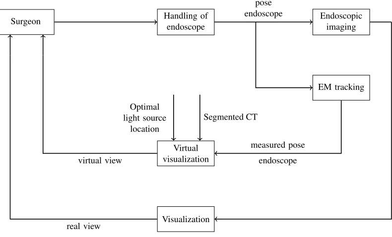
The designed system should fulfill all criteria as they are defined in section 2.2. The block diagram in figure 4 shows on a high level what actions define the functionality of the system and what data streams run in it.

Handling of endoscope

Surgeon Endoscopic imaging

EM tracking

Virtual visualization

Visualization

pose endoscope

Optimal light source

location

Segmented CT

measured pose endoscope

endoscopic images

virtual view

[image:10.612.120.515.377.616.2]

real view

(11)

With this diagram, the tasks the system should be able to perform on a functional level are defined. In order to create a system that shows an intuitive view of the real-time tracked endoscope data, these tasks need to be fulfilled according to the diagram:

1 Real time tracking of the endoscope, this includes:

– Calibration of the camera with respect to the coordinates of the tracking system

– Registration of the tracking tool with the coordinates of the CT data 2 Intuitive visual feedback of the position of the endoscope to the surgeon, this

includes:

– Creating a virtual view of the scene

3 Visible information about critical structures during the treatment, this includes:

– Segmentation of critical structures

– Creation of a virtual 3D model of the head of the patient and the segmented structures inside it

2.4 Functional architecture of a system for navigation in the

paransal sinuses

In order to provide the functionality that is demanded in section 2.3, some choices are made regarding the design of the system. This section describes the different possibilities and choices that were made, supported by the literature research that was conducted at the beginning of the project. The literature research can be found in appendix A.

2.4.1 Real time tracking

Real time tracking of the endoscope will be realized using an EM system. Another option was the use of an optical system. Due to two reasons the EM system is chosen: first of all this is the system that is used by the surgeons in the AvL hospital already, so it means that the least additional hardware is introduced in the operation room (OR). Second, this system can easily be read out and it is intuitive to manipulate and make simulations with. Some experiments are conducted on the optical system in order to make a comparison. Information about this system can be found in appendix B. In the literature research can be read that the accuracy of both systems is similar.

Other options of tracking the position of the endoscope in the nasal cavities are based on the video stream of the endoscope itself. These are the so called “volume from view” algorithms. Some options are for example: shape from shading [12]–[14]and structure from motion [15]–[17]. Other techniques are discussed in the literature research in appendix A.3.1 and A.3.2.

(12)

2.4.2 Intuitive visual feedback for the surgeon

An intuitive view can be achieved in many different ways. One is for example to augment the endoscopic view with additional information from a virtual view, as described in [18]. Another option is to only show the virtual view from the same viewing point as the endoscope. A third option is to show only a part of the patients head, and from an outside perspective, the movements of the tool inside it. The decision is made to investigate the latter two options. This choice is mainly made because there are less steps required in order to create this, and the functionality of merging the real and virtual endoscopic view can always be added later on if required.

2.4.3 Visible information about critical structures

Critical structures can be shown in various ways as well. Different options are an overlay on the endoscopic images, specific landmarks and distinctive colors for spe-cific tissue in the rendered view [19]–[22]. In this design the choice is made to make a spacial segmentation in the CT data files of the patient. These structures are dis-played in different colors and combined with the main patch in the rendered view. All anonymous CT and MRI data is available in the standard Digital Imaging and Communications in Medicine (DICOM) format.

2.4.4 Ideal light source location

In parallel with this project, another project concerning navigation during PDT is running in the AvL hospital. In that research a model is developed for reflection of light inside the nasal cavities, in order to determine the amount of light that reaches a specific surface. With this information the best location for the light source can be defined. The place where the most light hits the tumorous tissue and as little as possible light reaches the healthy tissue is considered the optimum. This location is calculated using a Matlab script and a DICOM data matrix. The location can be imported in the designed system, since it works on the same CT coordinate system. This location can be made visible in the virtual view.

2.4.5 3D visualization

(13)

• A display combined with the use of glasses:

– Stereo anaglyph

The differently colored left and right image are superimposed on each other. Typically the contrasting colors are blue and cyan. With corresponding colored glasses for the left and the right eye, the image that is intended for each eye can be seen. Prolonged use of this technique can cause headaches [25].

– Polarization

The light rays that compose the image are polarized. Light that is polarized in one orientation and light that is polarized in another orientation is superimposed. With the use of glasses that filter the light, the different images for the left and the right eye can be obtained. Disadvantage is the loss of half of the brightness of the image.

– Active shutter technique

The left and the right image are displayed sequentially. The glasses of the user shut the right and the left eye in matching frequency with the display. These glasses need some sort of power supply and are more heavy than the other two options.

• Autostereoscopic display (without the use of glasses): The left and right image are interlaced per pixel and an extra layer is placed in front of the display. Options are:

– Parallax barriers

The layer consist of precisely spaced slits. When the user is in a certain position, the slits make it possible to see a different set of pixels with each eye.

– lenticular lenses

The layer consist of lenses that magnify a different set of pixels when seen from a different angle. When the user is in a certain position one set of pixels reaches the left eye and the other set reaches the right eye, allowing them to see a different image.

• Head mounted display

Two displays are mounted in a headset, showing a different image to each eye. The disadvantage is that the user cannot decide when to look at the real world or at the screen. Either the real world is not visible, or in the case of see-through glasses, the virtual view is always seen against the background of reality.

Since the system will be used in the OR, having an extra set of glasses for the surgeon is not preferred. This might make the vision of the original endoscopic video less clear and therefore might introduce a risk during a surgical treatment. The same holds for a head-mounted display.

(14)

[image:14.612.108.505.70.180.2]

(a) Lenticular lenses (b) Parallax barrier

Figure 5: Auto stereoscopic display options [23]

The working principle of the two options for auto stereoscopic displays is given in figure 5.

2.5 Final architecture

The final architecture consist of parts that follow from the requirements and the design choices that are explained in the previous sections. The final design consist of the following parts:

• Segmentation

First the air is distinguished from tissue and later the eyes, optical nerve and the tumorous tissue are separated from the other tissue

• Camera calibration

In this step the camera is linked to the EM sensor that is attached to it, using a checkerboard pattern to define the world coordinates, and taking several images of it, combined with EM measurements. Also, the camera specifications, or ‘intrinsics’ matrix K, of the endoscopic camera is defined.

• Point registration

An initial registration is made using pinpointing on the model of the patient

• Surface registration

Fine tuning of the registration is performed with a surface registration on a patch of the model of the patient

• Real time camera positioning

Real time EM data and camera images enter the system. The calibration and registration matrices are used to calculate the position and orientation of the camera in the CT coordinate system.

• Displaying the rendered view

(15)

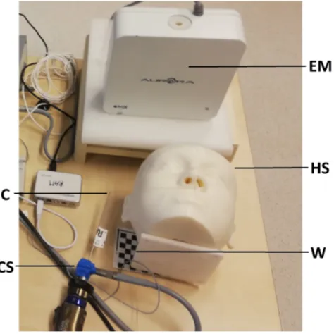
The different tools, sensors and other relevant parts of the system all have their own coordinate system. In order to be able to talk about the architecture, these different coordinate systems need to be defined first. The coordinate systems of the relevant parts of the system are the following and can be seen in figure 6:

• CS: Camera Sensor; sensor attached to the endoscope

When the EM system is used to find the position and orientation of the endo-scopic camera, this camera needs to be equipped with a sensor

• HS: Head Sensor; sensor attached to the head of the patient

The head of the patient should be tracked with a sensor as well, since in case it moves, the images should still be correct. If the head would not been tracked, the it can move with respect to the CT data, thereby destroying the registration of CT data with the EM system coordinates.

• T S: Tool sensor; sensor of the pre-calibrated tool

A pre-calibrated tool, is used for registration of the patient to its CT data via the EM system. This tool is more accurate than the endoscopic tip, because there is no calibration step involved which introduces errors.

• C: Camera

The endoscopic camera that is used throughout the procedure

• EM: Electromagnetic beacon

The reference of the electromagnetic tracking system

• CT: CT images of the patient

The virtual view is based on CT data and is displayed in CT coordinates

• W: Checkerboard pattern

[image:15.612.185.422.438.675.2]

The checkerboard pattern defines the world coordinate system

(16)

2.5.1 The transformation matrix

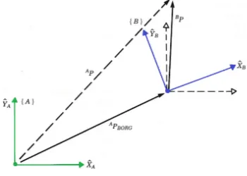
Different coordinate systems can be related to each other via rotation and translation of the origin. A certain point P can be expressed in frame b: Pb, to find this point in

systema,Pahas to be determined. If the rotation frombtoa,aRb, and the translation

of the origin:a_P

b,org are known, the new coordinates can be obtained. In figure 7 a 2D

[image:16.612.218.393.193.318.2]

example of the transformation of a point P in coordinate system A to the same point expressed in coordinate system B can be seen. The new coordinates are calculated as

Figure 7: 2D transformation from coordinate system A to coordinate system B

follows:

a

P = aRb bP + aPb,org

If the coordinates are expressed as homogeneous coordinates, which means that a 1 is appended at the end of the vectors, the rotation and translation can be combined in one matrix, the so called transformation matrix:

a_T b =       | a_R

b | aPb,org

|

− − − − −

0 0 0 | 1

     

The transformation with use of aTb looks like:

_a

P 1

= aTb _b

P 1

Some important aspects of transformation matrices are the following:

• To find the transform from c to a, when only the transforms a_T

b and bTc are

known, the transformation matrices can be multiplied in order to find the desired transformation:aTc= aTb bTc

• The inverse of the transformation matrix gives the inverse relation between the coordinate systems:a_T−1

b = bTa

(17)

2.5.2 Relating transformation matrices for the system

The system should be able to display the virtual endoscopic view from the same position and orientation as the real endoscopic view. The only real-time data available during surgery is the ‘real’ endoscopic view, the EM tracker data of the sensor attached to the endoscope and the data from the head sensor. The desired result is the CT data, seen from the position at which the camera ‘looks’ at the scene, or the camera coordinate system. The resulting transformation matrix is therefore: CT_T

C.

In order to realize this functionality an architecture of the system is made that shows how all different coordinate systems will be linked to each other and how the input is being processed and leads to the desired output. In the graph in figure 8 all coordinate systems and their relating transformation matrices are given. The blue arrows indicate data that can be measured directly, the black arrows are for data that can be derived from previous matrices and real-time measurements. The data on the green arrow is available from Matlab’s camera calibration. The red arrows indicate transformations that are not directly available. In order to find CS_T

C the calibration procedure is

needed and forHS_T

C the registration procedure must be performed.

C

CT

legend:

EM: Electromagnetic beacon W: World or checkerboard CS: Camera sensor

HS: Head sensor TS: Tool sensor, C: Camera CT: CT data W CS HS TS W_T C C_T CT =

CS_T−1

C EMT

−1

CS EMTHS HSTCT

CS_T

C

CS_T

HS = EMT_CS−1 EMTHS

HS_T

T S = EMTHS−1 EMTT S

[image:17.612.89.575.335.674.2]

HS_T CT EM EM_T CS EM_T T S EM_T HS EM_T W

(18)

2.5.3 Functional block diagram

[image:18.612.91.501.213.635.2]

All parts and coordinate transformations come together in one diagram: the functional block diagram in figure 9. It shows what actions the system takes (blocks) on what data streams (arrows).

(19)

3 Implementation of the system

This section describes how the tasks and system blocks are executed. The implementa-tion consists of transformaimplementa-tions from the EM sensor to the camera coordinate system and the visualization of this data in order to create a virtual view that matches the endoscopic view. Different transformations are made to find the real-time position and orientation of the endoscope. The main loop combines all underlying processes and links the different parts of the system to each other. First this main loop is described and then all underlaying processes are addressed.

3.1 Real time virtual camera positioning: main loop from

input to output

When the coordinates from the EM sensors enter the computer, this information has to be transformed into the position and orientation of the tip of the endoscope in camera coordinates. With the help of the calibration and registration steps all bits of information are available, and only a number of calculations needs to be performed in order to find the camera coordinates necessary for a virtual visualization.

When all pre-processes are finished, as can be seen in the block diagram in figure 9, the input of the system consists of:

• Calibration parametersC_T CS, K • Registration parameters CTTHS

• Real time EM data camera sensorEM_T CS(t) • Real time EM data head sensor EM_T

HS(t)

One real-time input is the matrix EM_T

CS(t), it gives the camera sensor transform in

EM coordinates. To find the transform of the endoscopic tip the camera calibration can be used:

EM_T

C(t) =EM TCS(t) CTCS−1

Another real-time input is the matrixEMTHS(t), together with the registrationCTTHS

the coordinates of the camera can be transformed to the CT coordinate system:

CT_T

C(t) =CT THS EMTHS(t)−1 EMTC(t)

The resulting transform is the desired CT_T

C, which contains the position and

orien-tation of the camera in the CT data coordinate system. This can be used to match the virtual view to the real view of the endoscopic camera. A visualization protocol is designed, which is described in section 3.2.3.

In pseudo code the main calculation is in algorithm 1.

3.2 Underlying processes

The main calculation loop makes use of inputs: calibration parametersC_T

CS and

(20)

Algorithm 1 Main Loop

1: Initialize 3D head model

2: connect to plusserver

3: while stopbutton 6= pressed do

4: input from plusserver:

5: EMTCS(t)

6: EMTHS(t)

7: EMTC ← CTTHS EMTHS−1 EMTCS CSTC

8: CTTC,ortho← orthogonalize CTTC

9: Output for visualization CTTC,ortho

10: end while

have to be defined beforehand, and the transformation matrix has to be converted into a visualization afterwards. This section describes the procedures that are used for these pre- and post-processes of the main loop.

Initially a 6-step procedure was developed in order to identify and link all coordinate systems. And to find the position and orientation of the endoscope expressed in the desired coordinates. This procedure started with estimating the transformation from the sensor on the endoscope to the tip: CS_T

t. This transformation would be

used throughout all steps where the endoscope was involved. This however, means a reduction in accuracy in comparison with the use of a pre-calibrated tool of the EM system. It also meant that the registration was dependent on the calibration. Two new, separated, step-by-step procedures were created in which the pre-calibrated tool (TS) is used whenever possible. The new 3-step procedure for calibration is given in section 3.2.1 and the procedure for registration is given in section 3.2.2. The original procedure can be found in appendix C.

3.2.1 Calibration: from EM sensor to camera coordinate system

This procedure describes how to find the transformation from the information of the sensor on the endoscope (CS) to the position and orientation of the endoscopic camera (C).

Step-by-step procedure for camera calibration

1 W_T

EM registration:

Registration of the EM coordinate system to the world coordinate system 2 W_T

C callibration:

Camera calibration to register the camera coordinate system to the world co-ordinate system

3 CS_T

C estimation:

(21)

Step 1: W_T

EM registration

The world coordinate system is defined by a checkerboard. In order to link this in-formation to the EM system, the corners of the checkerboard are touched with the pre-calibrated tool and these positions and orientations are saved. An algorithm to calculate the transformation from EM to W is used, for example Procrustes from Mat-lab [26]. This transformation is found by estimating a linear(translation, reflection, orthogonal rotation, and scaling) fit between the two input datasets. In this case the to sets of data are W_P_{; corner points in checkerboard coordinates and} EM_P_{; corner}

points in EM coordinates. The transform is hence:

W_T

EM =P rocrustes(WP,EMP)

Step 2: WTC calibration

A number of images of the checkerboard is taken using the endoscope, and the trans-formation of the sensor on the endoscope is stored simultaneously. The camera cali-bratior is started in order to find the corners in the images, and calculate W_T

C [27].

Step 3: CSTC estimation

As written in the previous step, when the pictures are taken also the EM position of the sensor of the endoscope is stored in the matricesEMTCS(i), wherei indicates the

ith _{image. With the use of the previously calculated matrices this can be transformed}

into the position of the tip in world coordinates using the following formula:

W

TCS(i) =W TEM EMTCS(i)

The transformation matrix to go from endoscopic tip coordinates to the camera co-ordinates can then be determined for every image:

C_T

CS(i) =C TW WTCS(i)

In order to find C_T

CS, the rotation and translation of the CTCS(i) matrices are

aver-aged.

(22)

Algorithm 2 Calibration protocol

1: input registration of EM system to checkerboard:

2: WPCH

3: EMPCH

4: WTEM ← procrustes(WPCH,EMPCH)

5: input Take images from checkerboard:

6: EMTCS(i)

7: F(i)

8: WTC ← Matlab camera calibration(F(i))

9: for i ← 1to 20do

10: WTCS(i)←W TEM EMTCS(i)

11: CSTC(i)←W TCS−1(i) WTC

12: end for

13: CSTC ← average(CSTC(i))

3.2.2 Registration

The registration procedure links the coordinate system of the electromagnetic head sensor (HS) to the coordinate system of the CT scan (CT), the result is the transfor-mation matrix:CT_T

HS.

Why using a head sensor

A model of the patients head is created with use of the pre-operative CT-data and the endoscopic tip will be registered to this model. As a part of this procedure, the real face of the patient or the phantom is touched with the endoscope. With one sensor this would be a rigid registration, depending on the location of the head or phantom in world coordinates. But during surgery or treatment, the head might move with respect to the world and the registration might lose accuracy. This problem can be avoided by adding an extra sensor to the system, and defining the registration matrix via this sensor. This sensor can be attached to the head and move along with it during surgery.

Point registration versus surface registration

In general two methods of registration are commonly applied in medical equipment, point-based registration [28] and point cloud based registration [29]. This is also called surface registration.

(23)

tip positions in the EM-coordinate system, with respect to the head sensor, to the points on the CT-model.

The second method is surface registration, a somewhat more cumbersome method to implement, but also more accurate. For this method a point cloud is defined, consisting of a part of the surface of the CT-model. The tool tip is moved around on this surface, and the data of its orientation and position in EM coordinates, with respect to the head sensor, is stored. Then an Iterative Closest Point (ICP)-algorithm is used to find the best CT_T

HS to match the two point clouds. ICP-algorithms are

used to minimize the distance between two point clouds. This is done by iteratively matching every point in the moving cloud with the closest point in the reference cloud and estimating the transformation that is needed to project the moving cloud onto the reference. This is done until the distance between the point clouds is below a set maximum.

Combination of forces

The best results can be gotten from ICP-algorithms if there exists a reasonable initial transformation [32]. In order to satisfy this condition and get the best possible reg-istration, a combination of both point registration and surface registration is made, consisting of three steps:

Step-by-step procedure for registration

1. Point registration CTTHS,init:

Make an initial transformation between the CT and the EM system using four predefined points

2. Surface registration CTTCT,init:

Iterate the ICP-algorithm in order to find an accurate match between the surface and the points registered by moving the EM tool on a (predefined) part of the surface

3. Total registration CT_T

HS:

Calculation of the transformation from the head sensor coordinates to the CT coordinates

These steps are translated into pseudocode in algorithm 3.

3.2.3 Visualization

(24)

Algorithm 3 Registration protocol

1: initialize 3D head model

2: connect to plusserver

3: Point registration

4: input reference points: CTPCS(i)i∈[1,4]

5: for i ← 1to 4 do

7: EMTCS(i)

8: EMTHS(i)

9: HSTCS(i)←EM THS−1(i)

EM_T

CS(i) 10: HSPCS,init(i)←HS TCS(i)[1 : 3,4]

11: end for

12: CTTHS,init← procrustes(CTPCS,HSPCS)

13: Surface registration

14: initialize Surface patch on 3D head model: pointcloudCTPCS(n); n ∈patch

15: while j < n do

17: EMTCS(j)

18: EMTHS(j)

19: CTTCS,init(k)←CT THS,init EMTHS−1(k) EMTCS(k) 20: CTPCS,init(k)←CT TCS,init(k)[1 : 3,4]

21: j + +, k+ +

22: end while

23: CTTCT,init← ICPalgorithm(CTPCS,CT PCS,init) 24: CTPCS ←CT TCT,init CTPHS,init

25: show registration on 3D head model

26: if User is satisfied then

27: CTTCS ←CT TCT,init CTTHS,init

28: output CT_T

HS

29: else

30: if More points required then 31: j ←1, go back to 15

32: else if New surface registration required then

33: j, k ←1, go back to 15

34: else if New point registration required then

35: go back to 5

36: end if

(25)

Segmentation

Air segmentation is performed in order to make a differentiation between the head of the patient and the air around it, as well as the cavities inside it. Further segmentation is done to emphasize critical structures and visualize anatomical landmarks of the bone structure. Typically both CT and MRI data are available for a sinus surgery and thus also for the succeeding PDT treatment.

A CT scan determines relative densities and expresses this in numbers on the Hounsfield scale, in Hounsfield Units (HU). Distilled water at standard pressure and temperature is defined as 0 HU. Air is defined as −1000 HU and soft tissue is around 100−300 HU. By using these numbers a segmentation of the CT data can be made by applying a threshold to the data. In figure 10 the difference can be seen between one slice of the original data and one slice where the distinction between air and tissue is made. The edges now show a sharp differentiation which can be used to generate a patch.

(a) Original data (b) Threshold is applied

Figure 10: Segmentation of air and tissue with use of a threshold value for the Hounsfield units

For the MRI images, on basis of visual inspection of the surgeon, a segmentation can be made as well. The structures that are chosen to be segmented from this data are: eyes from the CT, carotid arteries and tumor from the MRI.

Patch and filling of the model

The edge between air and tissue is used to generate a patch. The inside voxels of the head are filled in order to give a realistic as possible view of the scene.

Ideal light source location

When the ideal position and orientation of the light source is available it can be written as CT_T

light,ideal. If the light source is attached to the endoscope a transform

can be determined to relate the camera and the light source:C_T

light. Together with the

(26)

orientationlight,ideal_R

light(t), between the desired transform and the current transform

can be calculated:

CT_T

light(t) = CTTC(t) CTlight

Dlight(t) =||CTPlight,ideal − CTPlight(t)||2

light,ideal

Rlight(t) = CTR_light,ideal−1 CTRlight(t)

These values can be shown on screen in order to inform the surgeon about the prox-imity of the ideal location.

Virtual endoscopic viewpoint: the pinhole camera model

Figure 11: Pinhole camera model The virtual endoscopic viewpoint should

match the real endoscopic viewpoint, but also give additional information if pos-sible. Information of the real camera is used to define the parameters of the vir-tual camera.

The so-called pinhole model of an optical camera is used. An image of this model can be seen in figure 11. The camera coordinate system (C) is based on this model. The origin is the focal point of the camera, this is the pinhole or camera center. The z-axis is the optical axis by definition. The x-axis is usually the hor-izontal axis and the y-axis is vertical. If

the image is considered to be a matrix, thexvalues are the rows and theyvalues are the columns.

Figure 12: Skew α

The z-axis intersects the image plane orthogonally at dis-tance d, this is the focal distance, thus the image plane is parallel with the xy-plane. If the x and y axis are not or-thogonal to each other, a skew coefficient is also included. In figure 12 can be seen what the effect of skew is.

(27)

Intrinsics

Part of the intrinsics of a camera are combined in the matrix K and include focal length, the principal point and the skew coefficient. The other intrinsics are distortion parameters. An ideal pinhole camera does not have a lens and therefore it does not include distortion. However, the endoscopic camera does have a lens, so distortion parameters are also relevant.

In order to generate a rendered view that matches the real endoscopic view as accu-rately as possible, all camera intrinsics should be applied to the model. On the other hand, in order to have a view that shows as much and as clear information about the real situation as possible, distortion and skew might be deformations that should not be included. The focal length and the principal point define how wide the angle of view is, that means that these parameters decide what will fit in the image and what will not. To match the view, this should be the same for rendered and real, but maybe it is preferable to see more (or less) than what is on the actual endoscope’s display. Because of these considerations, the intrinsics of the camera are calculated, but application is limited to adaptation of the camera angle.

Extrinsics

The extrinsics of the camera viewpoint consist of the position and orientation of the camera in another frame than the camera system coordinates. From camera calibra-tion in Matlab the transformacalibra-tion from C to the checkerboard, or W frame can be found. The calculations of the calibration then make it possible to get the transfor-mation from the camera sensor(CS) to the camera (C). Finally when the registration parameters are applied, the position of the camera in CT coordinates can be found this gives the matrix:CT_T

C,ortho. This gives the position and orientation of the virtual

camera in the CT coordinate system.

Outside viewpoint: 2D visualization of the endoscope

The extrinsics of the camera are used to position a model of the endoscope within the virtual view. The head is partially shown, in order to be able to see the cavities on the inside. The model of the endoscope is based on the real dimensions of the 0◦, 4 mm Karl Storz rigid endoscope.

3D visualization

Since autostereoscopy was chosen to be the most suitable solution for 3D in the OR, an autostereoscopic display was obtained from the company Dimenco [33]. This company is at this point in time one of the only companies investing in 3D technologies. Larger autostereoscopic displays for medical use are under development.

(28)

4 Realization

In order to realize the system, hardware components and programming solutions are chosen, to fulfill the desired tasks. This section describes the physical realization of the building blocks of the system.

4.1 Hardware components

[image:28.612.89.522.338.563.2]

The physical setup consist of several parts: the EM tracker system, a laptop with the Matlab code on it, a phantom of a patients head, an endoscope with camera connected to the laptop via a framegrabber from Terratec, an EM tool, a head sensor and a sensor that is attached to the endoscope. A checkerboard pattern is necessary for the calibration with respect to the world coordinate system. The table where the setup is placed on may not consist of too much metal, since this disturbs the magnetic field of the tracker system. In case this is unavoidable, some plastic spacers are used to move the EM field further away from the table. In figure 13 the combination and connection of the different parts can be seen. All relevant parts will be discussed in the following sections.

Figure 13: Setup diagram

4.1.1 Phantom

In order to test the code during the process, and to perform experiments, a phantom was created especially for this research at the very beginning of the project. DICOM data of an anonymous patient of the AvL was used for this purpose.

(29)

[image:29.612.306.522.111.371.2]

CT data could be made, differentiating tissue from cavities.

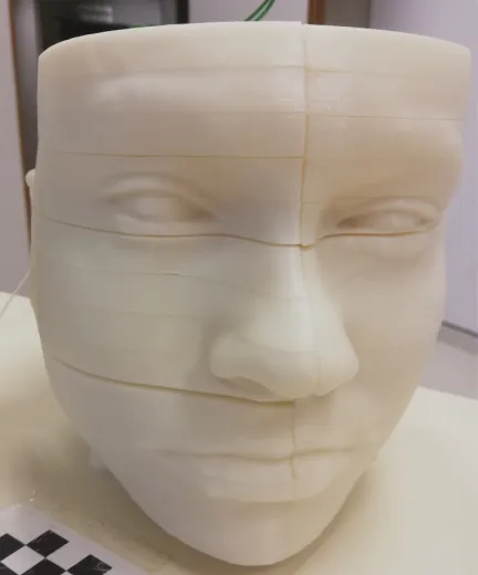
Figure 14: The 3D printed phantom The segmentation was loaded into

soft-ware called meshmixer, in order to cre-ate a 3D model of the head, excluding the cavities [34]. 3D printing is only pos-sible when the model consist of one part, no loose pieces can be involved. Also, if any loose parts exist his is caused by in-accuracies of the model, since there are no floating parts in anyone’s head. With use of Netfabb the model was tested for print-ability and the loose parts were de-tected and deleted.

To make the phantom useful for testing the code, it is an advantage to be able to look inside it, in order to visually match the real and the virtual views. To sim-plify this, the model was vertically cut in half and horizontally cut in 14 slices, which were all printed separately. Four recesses were made into the model, to be able to put it on four poles and keep the parts together.

The model is 3D printed using Acrylonitrile Butadiene Styrene plus (ABSplus) P430 in the color ivory. This material is right for an in-vivo experiment because of its light scattering properties, which are comparable to those of mucosal tissue, as measured, on white ABS,with a setup in the AvL hospital [35].

Figure 14 shows a picture of the phantom. In appendix D.2 a manual can be found for creating smooth, evenly spaced, slices of a model with the use of meshmixer.

4.1.2 Checkerboard

The world coordinate system is defined by a 9x6 corners checkerboard pattern with 10x10 mm squares. One direction needs an odd number of squares and one an even, because Matlab can then easily define the x and y directions. This is printed and stuck to a plastic spacer in order to prevent it from moving during the experiments.

4.1.3 Head sensor

(30)

4.1.4 Sensor attached to the endoscope

Figure 15: Coordi-nates of the 6DOF EM sensor, all di-mensions are in mm The sensor that is attached to the endoscope is a standard

6 degree of freedom (DOF) sensor from the EM system. The coordinate system associated with this sensor can be seen in figure 15 [36].

4.1.5 Framegrabber

In order to establish the connection between the endoscope tower and the computer, a “framegrabber” or analog-to-digital converter was used. This is the grabster AV300 from TerraTec, which was connected using a composite cable. It has a framrate up to 29 fps. With software from TerraTec and Matlab code, the “grabbed” images could be loaded into the design.

4.2 Code of the software

This section shows how the different procedures that are de-scribed in the implementation are realized in code.

4.2.1 Programming language

As is mentioned before, Matlab is used for all the code parts of the system. This is the most convenient choice, since some parts like the connection protocol with the plusserver and a camera calibration toolbox, were already available in Matlab. Also, code for additional algorithms could easily be found and implemented as will be described in the next sections.

A large part of the designed system consist of matrix calculations of transformations on datasets such as the CT data. Matlab is specifically good at matrix manipulation, its linear algebra routines are powerful and simple to use with often only very few code. For example, matrix calculations with inverses can elegantly be coded, the original implementation inv(A)∗B is suggested to be replaced with the faster: A\B.

Figure 16: 3D filling of the head model

4.2.2 Patch and filling of the model in Matlab

(31)

the idea of looking inside some tissue. To resolve this problem, the algorithm vol3d is used [38].

Dependent on the normalized Hounsfield value a specific shade of a chosen color scheme is used to fill the voxels inside the patch. In figure 16 the model of the head can be seen from above.

4.2.3 Segmentation of critical structures

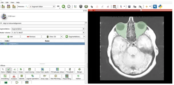
[image:31.612.156.460.263.412.2]

The segmentation of the chosen structures is done with the program 3Dslicer [39]. This program is able to automatically segment bone, but other sorts of tissue have to be manually segmented. In figure 17 a screenshot of the program, with a slice of a MRI scan with roughly segmented eyes can be seen.

Figure 17: Screenshot of segmentation with 3D slicer

The data of the MRI and the CT scan need to be matched in order to be able to show this information on the same screen, this is also done with 3dSlicer. The segmentation is stored in a stl file, just like the original greyvalues, which is loaded into Matlab to define the CT-model of the critical structures in the head.

The visualization of the segmented tissue is also done by generation of a patch. These patches have different colors from the head patch, in order to emphasize their presence and importance during a treatment. In figure 17 a combination can be seen of the segmentation of the eyes and the tumor, against the background of a transparent patch of the total head.

4.2.4 Calibration

The realization of the calibration protocol follows the steps that are described in section 3.2.1.

Checkerboard registration

(32)

[image:32.612.220.406.91.236.2]

Figure 18: Patches of the segmentation of the eyes and tumor in Matlab

to put the tooltip on the first corner and click “ok”. When this is done the user is asked to do the same for the second corner and so on until the 54th(if a checkerboard with 9x6 corners is used). When taking the positions of the checkerboard corners, an average of 50 measurements is taken in order to minimize the positioning error. Matching of the EM data with the world data, that is; the defined coordinates of the checkerboard corners, is performed with the Matlab algorithm Procrustes. This algorithm minimizes the sum of squared errors between the original points and the transformed points after registration: W_P

reg =W TEM EMPreg.

Taking images of the checkerboard

The next step is to take images from the checkerboard with the endoscopic camera, while saving the position of the sensor on the endoscope. For this the user is asked to hold the endoscope in a specific position, and press “ok”. At that moment a snapshot of the endoscopic video is taken, using the framgrabber and the Matlab plug-in, and the position of the sensor is stored in a vector. Before starting to take images, the user has to enter the amount of images that will be taken. When all images are done, the user is asked to start the camera calibration app of Matlab and enter the images in there. When the calibration is performed, usually some images are left out because they are not good enough.

Combination of inputs

All pieces of information are combined in the final part of the code, where the actual calibration calculation takes place. The user has to enter the numbers of the images that are used for camera calibration. The tracker data should only be used from the instances of which there is a picture as well. The transformations from the camera coordinates to the camera sensor coordinates are calculated via the world coordinate system defined by the checkerboard.

The pointsW_P

(33)

the checkerboard. The mean squared error gives the distance between the individual origins of CS_T

C(i) and their average. If all calculated matrices lay far away from the

average, the average is less likely to be correct. If only one value is added or deleted, the mean changes a lot. A high RMSE has therefore less impact if more measurements are taken. Adding or removing one measurement, even if it has a large differentiation from the average, has less effect on the outcome.

4.2.5 Registration

Point registration

For the initial point registration, four points are chosen on the surface of the patch of the head. For accuracy it is recommended to choose feature points of the face, like eye corners, mouth corners, sides of the nostrils etcetera. This is in order to be able to point at the exact same location on the phantom as is indicated on the patch. In figure 19a an example of four points is shown. When the user wants to define the points himself a separate program can be started and the user can indicate as many points on the patch as he desires for the registration. The predefined points on the CT patch are matched to the stored positions of the tool in EM coordinates with use of the Matlab algorithm Procrustes.

(a) Initialization of surface registra-tion with 4 points

(b) Part of the patch that is used for surface registration

Surface registration

When the point registration is done, the surface registration is started. For this a separate patch is loaded that only consists of a specific outside part of the face. This patch can be seen in image 19b. The user moves the tool around on this area of the head of the patient and the positions of the toolsensor EM_T

CS are stored in a vector,

(34)

functionalities. For example the Matlab algorithm pointCloud finds a rigid transform without scaling, as well as rigidICP but ICP finite has more options. All three, and a combination of the rigid and the scaled algorithms were tested and compared in order to get the most accurate results. These results were very much equal for affine transformations, so the ICP finite algorithm is used with the option “affine” [40].

4.2.6 Virtual endoscopic viewpoint

[image:34.612.348.520.257.367.2]

The virtual view can be seen as the view through a pinhole camera, and as such it has intrinsics and extrinsics that can be set.

Figure 20: Schematic representa-tion of camera angle α in x-direction

Intrinsics

The only part of the camera intrinsics that can be easily influenced in Matlab iscamva, the viewing angle of the camera. To determine this value, the intrinsics that follow from the camera calibration in section 3.2.1 are used. In figure 20 a schematic representation of the camera intrinsics is given. It can be seen that the viewing angle α depends on the focal length expressed in pixels: d∆ and the image size N∆. Where ∆ is again the pitch, or distance between pixels in mm. This distance is assumed to be equal for the xand y direction, so ∆x = ∆y = ∆.

To calculate the viewing angle a simple applica-tion of Pythagoras’ theorem in both direcapplica-tions suffices:

αi =tan−1

1/2Ni∆

di∆

=tan−1

Ni

2di

i=x, y

In Matlab only one value can be set forcamva, so the maximum ofαxand αy is used.

Extrinsics

In Matlab a pinhole camera model is present of which the extrinsics can implicitly be set. This is done via the vectors campos, camtarget and camup. These respectively hold the position of the camera, the target where the camera is “looking at” and the vector that defines which axis is pointing upwards.

The position and orientation of the camera is found via the procedure as described in section 3.1 and given in CT_T

C. In order to apply this information to the camera

model in Matlab, the resulting camtarget and camup need to be defined.

(35)

scene. Starting from the “zero” orientation, the axes of the camera correspond to the axes of the ct view. In this case −y is pointing upwards and the viewing direction is z. So, the starting values are camup = [0 −1 0] and camtarget = [0 0 1] with campos= [0 0 0]. In order to create the virtual view that matches the real view, the orientation and translation are applied to the zero position, as follows:

campos← CT_T

C,ortho [0 0 0 1]T

camtarget← CT_T

C,ortho [0 0 1 1]T

camup← CT_T

C,ortho [0 -1 0 1]T

4.2.7 Main loop for real-time 2D endoscopic view

In Matlab a virtual camera is defined and updated with the new extrinsics from the main calculation loop. With the virtual endoscopic viewpoint protocol the 2D view of the virtual camera is shown real-time.

4.2.8 Main loop for real-time 2D visualization of the endoscope in the

model

The main calculation loop is used to position the model of the endoscope in the 3D model of a part of the head of the patient. The viewpoint is kept equal throughout the treatment, only the endoscope moves in this virtual view.

4.2.9 Main loop for 3D visualization

For generation of a 3D video, a recording is made of all the transformations of the camera sensor and the head sensor during a user-specified period of time. After the treatment or experiment, a movie can be created that can be played on a 3D screen.

In order to generate 3D data, two images are made, one for the left eye and one for the right. This is done by moving the position of the virtual camera and itscamtarget. To create 3D content some rules of thumb apply in the case you are taking images of a normal scene. These consist of placing the two camera positions eye distance apart and let the camera axes, the lines through campos and camtarget, cross on the position of the object that should appear “on screen”. Objects that are further away appear to go into the screen, closer objects seem to float in front of it. For endoscopic surgery these rules do not apply, since the field of view is very narrow and the distance between the camera and the objects of interest is very small. The solution is to place the virtual camera’s apart by only a small distance and letting the axes cross at some point closer to the camera position. Visual inspection is performed for different settings, and the best looking one is with the distance between the positions 1 voxel and the intersection at 5 voxels from the positions.

(36)

5 Experiments

In order to asses the quality of the delivered design, some experiments are conducted. These experiments are: visual inspection, assessment of error measures, Monte Carlo analyses and real-time performance tests.

5.1 Goal

The goal of the assignment is to make a protocol of programs that together form an accurate and intuitive navigation platform for a surgeon during a PDT treatment of the nasal cavities. In order to quantify when the system is accurate, some subgoals are defined with respect to five area’s of interest:

1 Accuracy and limitations of tool tracking

2 Accuracy of the registration of an electromagnetic sensor to CT coordinates 3 Accuracy of camera calibration

4 Quality of visualization

5 Real time character of the solution

5.1.1 Accuracy and limitations of tool tracking

The specifications of the EM system define the accuracy of the positions and rotations of the sensors, dependent on the distance from the EM generator. Metal objects in the field can cause a distortion of the signal. To be able to keep track of the precise location of the endoscopic tip, somewhere on the endoscope, which contains a lot of metal, a sensor needs to be attached. At first the extra distortion of the endoscope needs to be determined and then it must be minimized; the associated goal is therefore:

Subgoal 1

Minimizing the influence of the distortion introduced by the attachment of a sensor to an endoscope, which contains a lot of metal

5.1.2 Accuracy of the registration of an electromagnetic sensor to CT

coordinates

The accuracy of the current system is about 1,5 mm for registration of the EM tool to the CT coordinates. Other navigation systems for the nasal cavities also have sub 2 mm accuracy[41]. The proposed system should be comparable to existing systems, therefore the subgoal on this area of interest is:

Subgoal 2

Sub 2 mm accuracy for the registration from electromagnetic sensor to CT coordinates

5.1.3 Accuracy of camera calibration

(37)

for this calibration should be as small as possible, in order to make the total system as accurate as possible. Therefore the demand is sub 1 mm accuracy:

Subgoal 3

Sub 1 mm accuracy for the camera calibration transformation matrix from camera coordinates to camera sensor coordinates

5.1.4 Quality of visualization

The goal for the quality of the visualization is twofold. At one hand the requirement is that the rendered view gives a more clear visualization of the situation than the real view, at the other hand it should be matched accurately to the real viewpoint.

The first part seems to be entirely dependent of the opinion of the user, but can at the same time be quantified by the amount of information that is added to the virtual scene. The second part is dependent on the accuracy of the registration and calibration and can therefore be quantified using the criteria of subgoals 3 and 4 as well as a new criterium of the combined protocol. Since the system will be used in the OR and be looked at by surgeons, the visual comparison of the real and the endoscopic view also can give an indication of the quality.

Subgoal 4a

Improvement of the clarity of the situation in the virtual views compared to the real view

Subgoal 4b

Accurate match between the real endoscopic output and the virtual view

For the 3D view an extra requirement arises. The virtual 3D view of the scene should be generated in a way that the depth of the cavities is realistic. It must give an intuitive representation of the real situation.

Subgoal 5

Intuitive representation of the depth of the cavities when using the 3D visualization

5.1.5 Real time character of the solution

(38)

Subgoal 6

Maximum mean computation time of 0.15 seconds for one iteration of the loop from input to output in Matlab

The registration of the CT scan with the EM system has to be done during surgery, since the patient or phantom is needed to do this. Since the surgery should not be slowed down considerably by the use of this system, a limit for the total time of the registration is set:

Subgoal 7

Total time necessary for registration of the CT data to the head sensor coordinate system less than 5 minutes

5.2 Method

5.2.1 Setup

The hardware components of the setup are described in the section 4.1. The setup consist of: the EM tracker system, a laptop with the Matlab code on it, a phantom of a patients head, an endoscope with camera, connected to the laptop via a framegrabber from Terratec, a checkerboard pattern, an EM tool, a head sensor and a sensor that is attached to the endoscope. In order to check whether the subgoals are met, the following experiments are conducted, with in brackets which subgoal can be tested with this particular experiment:

• Visual inspection (4a, 4b, 5) • Error measures (2,3)

• Monte Carlo analysis (1,2,3,4b) • Time performance tests (6,7)

All experiments are carried out in the simulated OR of the University of Twente.

5.2.2 Statistical data processing

All experiments, except the visual inspection, can somehow be quantified. This section describes how the errors are calculated and how they can be interpreted. Also, the input errors for the Monte Carlo Analyses are discussed.

Error measures

When a registration is performed from one coordinate system onto another, the fidu-cial registration error (FRE) can be calculated. This is a measure that is often used to indicate the accuracy of the registration. It is the root mean square error in alignment of the fiducial points in one coordinate system and the projections from the points in the other coordinate system onto the first. This means that a measure for the difference between reference points and mapped measured points using the estimated mapping is calculated.

(39)

coordinate system b are b_P₍_i_{) and the estimated mapping is} a_T

b,est, the estimated

reference point positions are:

a_P

est(i) =aTb,est bP(i)

Then the FRE for n points is calculated as:

F RE =

v u u t

i= 1 n

n X

1

(a_P

est(i)− aP(i)).2

For all calculations with vectors P the dot-square means the element-wise square of the vector.

Another error measure is the root mean squared error (RMSE) itself. The estimated matrix for camera calibration, is an average of all of the outcomes. With the RMSE of these matrices with respect to the average, a measure for accuracy of the estimate can be given. When it is small, the measurements are consistent and the resulting matrix is very likely to be correct. Whereas if this number is larger, there must be some larger errors in the measurements, causing the resulting matrix to be less accurate. However, the more pictures are taken into account, the less influence the inaccuracy of the individual matrices have as long as the mean error is zero, as will be addressed further in section 5.3.2. If the average matrix a_T

b and all individual matrices aTb(i)

are known, when focusing only on the translation, the RMSE for n matrices is:

RM SEtranslational = v u u t 1 n n X i=1

(a_P

b − aPb(i)).2

When for example in a simulation, multiple times an estimate is made of the same matrix for which the true one is known, the RMSE can be calculated in exactly the same way as for the average and the individual estimates. Only now the result gives a measure for the average distance from the true translation.

Until now, only the translation from the transformation matrix is taken into account. When the focus is on the partaRbof the transformation matrix, the change in rotation

between the estimate and the real matrix can be found by multiplying with the inverse:

b,true_R

b = aRb,true−1 a_R

b

By transforming this matrix into an euler angle b,true_E

b the root mean squared error

can be calculated again for n matrices:

RM SErotational= v u u t 1 n n X i=1

(40)

Error measures for calibration

The FRE for registration of the checkerboard, which is the world coordinate system, with the EM coordinate system, can be calculated using the known locations in world coordinates of the checkerboard corners w_P

ch and the reprojected measured points:

W_P

ch,est(i) =W TEM,est EMPch(i)

Then the FRE for k checkerboard corners is calculated as:

F REwP ch =

v u u t

i= 1 k

k X

1

(w_P

ch,est(i)− wPch(i)).2

The FRE of the W_T

C matrices and the estimated matrices using the CSTC estimate,

can also be calculated because there are measurements available forWTC. When WTC

are the matrices that are measured and calculated with the camera calibration app, and W_T

C,est(i) =W TEM,est EMTCS,est(i)CSTC from the camera calibration procedure,

the FRE for the n pictures is:

F REwP e = v u u t

i= 1 n

n X

1

(w_P

C,est(i)− wPC(i)).2

The RMSE of the individual resulting matrices CS_T

C(i) with respect to the averaged

matrix, CS_T

C, can be calculated. Only the translation is taken into account:

RM SEcsP c= v u u t 1 n n X i=1

(CS_P

C− CSPC(i)).2

With a simulation, also the true CSTC,true can be compared to the estimated CSTC

for every m iterations of the simulation.

RM SEcsP c= v u u t 1 m m X i=1

(CS_P

C,true− CSPC(i)).2

RM SEcsRc = v u u t 1 m m X i=1

(C,true_E C).2

Error measures for registration

The point-registration of the phantom to the CT data is performed as described in section 3.2.2, four points are registered in order to initialize the surface registration. The FRE is calculated for the chosen points on the model of the CT data: PCT,ini,ref

(41)

the scaling factor between the model and the EM points. This is used in order to get the error in mm instead of voxel size. The calculations are:

PCT,ini(i) = CTTHS,ini PHS,ini(i)

F REctP hs,ini =

1 g v u u t

i= 1 4

n X

i=1

(PCT,ini,ref(i)−PCT,ini(i))2

Surface registration gives an error measure as well, since it tries to minimize the distance between the projection of the measured points and the surface. The error that results from this algorithm can usually be set to a maximum, in order to specify for how long the algorithm should continue with iterating, before accepting the transform. This is usually set to 0.001 mm. This error measure is however not so meaningful since there is no unique match of the measured points and the given surface. The surface consists of many more points than the registration, and since scaling by IPC is allowed, the points can easily be matched to a wrong part of the surface and still be within limits. This is typically caused by an initialization that is far from accurate.

When a simulation is done, the points on the surface where the measured points should be matched to are however known as PCT. For a simulation the registration

error between the target locations and the reprojections of those can be calculated. This is called the target registration error (TRE) and computed in the same way as the FRE. The errors should be calculated in mm, so the scaling factor from the head sensor to the CT system should be taken into account. This can be calculated with

p

det(HS_T

CT).The points PCT,ref(i) are known from the simulation.

PCT(i) = CTTHS PHS(i)

T REctP hs =

p

det(HS_T CT v u u t 1 n n X i=1

(PCT,ref(i)−PCT(i))2

With a simulation, also the trueCT_T

HS can be compared to the estimatedCTTHS for

every m iterations of the simulation.

RM SEctP hs = p

det(HS_T CT) v u u t 1 m m X i=1

(CT_P

HS,true− CTPHS(i)).2

RM SEctRhs = p

det(HS_T CT) v u u t 1 m m X i=1

(CT,true_E HS).2

Error measures for calibration and registration combined

Navigation for PDT in the paranasal sinuses using virtual views