Perceptual categorization

A Thesis Submitted for the Degree of PhD at the University of Warwick

http://go.warwick.ac.uk/wrap/36672

This thesis is made available online and is protected by original copyright. Please scroll down to view the document itself.

Perceptual Categorization Neil Stewart

Thesis submitted for the degree of Doctor of Philosophy

Department of Psychology University of Warwick

Table of Contents

List of Figures

List of Tables

Acknowledgements

Declaration

Abstract

Contents

11

v

x xu

Xlll

Contents n ..

Table of Contents

Chapter 1: Introduction ₁

Exemplar Models of Categorization ₄

Parametric Models of Categorization 9

Empirical Evidence for Exemplar and Parametric Models of 17 Categorization

The Relationship between Exemplar and Parametric Models of 24 Classification

Conclusions

26

Summary of Remaining Chapters 27

Chapter 2: The Effect of Variability in Perceptual Categorization 29

Abstract 30

The Effect of Category Variability in Perceptual Categorization 31

Modeling Sensitivity of Category Variability 39

Experiment 1 48

Experiment 2 52

Experiment 3 55

Experiment 4

66

Experiment 5 71

General Discussion 75

Appendix 80

Chapter 3: Identification and Categorization of Simple Perceptual Stimuli: A 81

Abstract

Difficulty in Determining Absolute Magnitudes

What Information is Used in Categorization?

The Memory and Contrast Strategy Modeling

Overview of Experiments

Experiment 6

Experiment 7

Experiment 8

General Discussion

Chapter 4: Feature Creation in Perceptual Categorization

Abstract

Feature Creation in Perceptual Categorization

Evidence for the Creation of New Functional Features

Evidence that New Functional Features Qualitatively Change

Perception

Overview of Experiments

Experiment 9

Experiment 10

Experiment 11

Experiment 12

Experiment 13

Contents v

List of Figures

Figure 1. The stimuli and the five category structures used by Ashby & 20 Maddox (1992).

Figure 2. The four category structures used by Nosofsky (1986). 21

Figure 3. The four category structures used by Nosofsky (1989). 21

Figure 4. A one dimensional example of two categories differing in 31

variability.

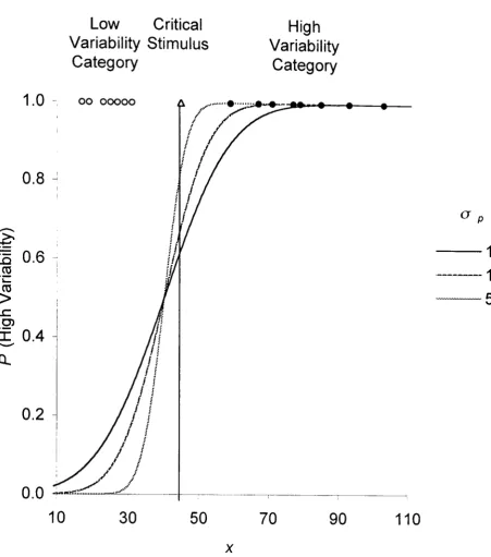
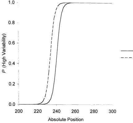
Figure 5. The probability of a high variability category response as a 41 function of the position of the stimulus on either dimension for normal GRT.

Figure 6. The probability of a high variability category response plotted as a 42

function of the position of the stimulus on the dimension for GCM (g=2).

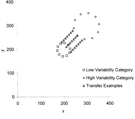
Figure 7. The arrangement of examples for the 1:2 pair of categories. 43 Figure 8. The arrangement of examples for the 1:4 pair of categories. 43

Figure 9. The probability of a high variability category response for an 44

example on the line Y=K-plotted against the X value of the absolute position

of the example for normal GRT for two categories (pair 1 :2), one twice as

variable than the other.

Figure 10. The probability of a high variability category response for an 44

example on the line Y K-plotted against the X value of the absolute position

of the example for normal GRT ~= 1 0) for two pairs of categories, pair 1:2

and pair 1 :4.

Figure 11. The probability of a high variability category response for an 44

to the nearest neighbor of the low variability category for normal GRT

(~= 10) for the 1:2 and 1:4 pairs of categories.

Figure 12. The probability of a high variability category response for an 45

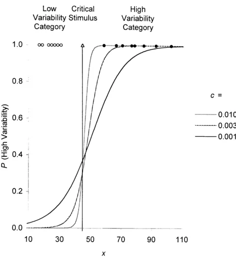
example on the line y K..plotted against the K value of the absolute position of the example for the GCM (g=2, [=2, ~=0.05) for two category pairs 1:2 and 1:4.

Figure 13. The probability of a high variability category response for an 45

example on the line y K..plotted against the K value of the example relative the nearest neighbor of the low variability category for the GCM (g=2, r=2,

~=0.05) for category pairs 1:2 and 1 :4.

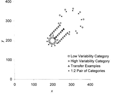
Figure 14. The arrangement of examples for the 1:2 expanded pair of 46 categories.

Figure 15. The probability of a high variability category response for an 46 example on the line y K..plotted against the K value of the absolute position

of the example for the GCM (g=2, [=2, ~=0.05) for two pairs of categories

1:2 and 1:2 expanded.

Figure 16. The probability of a high variability category response for an 47

example on the line y K..plotted against the K value of the absolute position of the example for the GRT ~= 10) for two pairs of categories 1:2 and 1:2

expanded.

Figure 17. The generalization gradients obtained from Experiment 3 for the 62

pairs of categories 1:2 and 1 :4.

Contents \11

pairs of categories 1:2 and 1 :4. The relative position is measured relative to

the nearest exemplar of the low variability category.

Figure 19. The generalization gradients obtained from Experiment 4 for the 69 pairs of categories 1:2 and 1:2 expanded.

Figure 20. Ten stimuli distributed evenly along a single psychological 87

dimension, divided into two categories.

Figure 21. The predictions for the MAC model for the simple category 89 structure illustrated in Figure 20. Accuracy for a stimulus on trial n is plotted

as a function of the stimulus on trial n-l.

Figure 22. The predictions for the GCM for the simple category structure 90 illustrated in Figure 20. Accuracy for a stimulus on trial n is plotted as a

function of the stimulus on trial n-l.

Figure 23. The proportion of correct responses for same category tone pairs 94

(1 ~5 and 1 0~6) and different category pairs (1 ~6 and 1 0~5) for

Experiment 6.

Figure 24. The stimulus structure used in Experiment 7 compared to

Nosofsky's (1985) stimulus structure.

97

Figure 25. The proportion of correct responses for same category stimulus 98

pairs (1 ~5 and 1 0~6) and different category pairs (1 ~6 and 1 0~5) for

Experiment 7.

Figure 26. The proportion of correct responses for same category tone pairs 102

(1 ~5 and 1 0~6) and different category pairs (1 ~6 and 1 0~5) for the

Figure 27. The average error on identification trials plotted as a function of 103 the preceding stimulus for Experiment 8.

Figure 28. The Martian cell stimuli used in the learning and verification 126 phases of Experiment 9.

Figure 29. The Martian cell snapshot stimuli used in the transfer phase of 127 Experiment 9.

Figure 30. The Martian cell stimuli used in the learning and verification 131 phases of Experiment 10.

Figure 31. The Martian cell snapshot stimuli used in the transfer phase of 131 Experiment 10.

Figure 32. The lines stimuli used in the training phase of Experiment 11. (a) 136

The two elements. (b) Examples of training stimuli.

Figure 33. The lines stimuli used in the transfer phases of Experiment 11. 136 Figure 34. The proportion of type AB responses for the single transfer 141

stimulus A'B as a function of the awareness that the compound is made from

the parts for Experiment 11.

Figure 35. The proportion of type AB responses for the single transfer 141

stimulus A-B as a function of the awareness that the compound is made from

the parts for Experiment 11.

Figure 36. The proportion of type AB responses for the single transfer 141

stimulus A'-B as a function of the awareness that the compound is made

from the parts for Experiment 11.

Contents IX

Figure 38. An example stimulus set from Experiment 12 (generated from the 144

prototypes in Figure 37).

Figure 39. The mean proportion of correct responses for the transfer stimuli 157 in Experiment 14. (Error bars are standard error of the mean.)

Figure 40. The mean proportion of correct responses for the transfer stimuli 165

in Experiment 16. (Error bars are standard error of the mean.)

Figure 41. The mean proportion of correct responses on trial

n

n-1

the opposite category for Experiment 3.

Figure 42. The mean proportion of correct responses on trial

n

of whether the distant stimulus on trial

n-l

the opposite category for Experiment 4.

Figure 43. Two separable categories, where one category is more variable 179

than the other.

Figure 44. The probability of a correct response as a function of the value of 180

the stimulus on the single dimension.

Figure 45. The mean probability of a correct responses on trial

n

function of whether the distant stimulus on trial

n-l

category or the opposite category.

Figure 46. Two conditions where the spacing of trials varies.

Figure 47. Displays controlling for the location of features across two

conditions of the proposed Study 6: within object and between object.

189

List of Tables

Table 1. Means across all three blocks for Experiment 1.

Table 2. Means across all three blocks for Experiment 2.

51

54 Table 3. Mean proportion of high variability responses across all participants 61

for Experiment 3, split by variability condition.

Table 4. Mean proportion of high variability responses across all participants 68

for Experiment 4, split by variability condition.

Table 5. Stress and

r2

the three different category structures.

Table 6. The mean inter-stimulus distance within a category derived from 73

the MDS solution.

Table 7. The GCM's predictions for summed similarity for different f 74

parameters.

Table 8. Mean proportion of responses for the transfer block of Experiment 130

9.

Table 9. Mean proportion of responses for the transfer block of Experiment 130

9 for those participants performing significantly above chance on types A, B

and AB in the transfer phase.

Table 10. Mean proportion of responses for the transfer block of Experiment 132

10.

Table 11. Transfer stimuli from Experiment 11. (a represents element a, b 136

represents element b, a' represents the mirror image of element a, b'

Contents Xl

were added to the stimulus. - is used to represent two stimuli being displayed

simultaneously, ---7 is used to represent two stimuli, the first displayed before

the second.)

Table 12. Mean proportion of responses for the single stimuli transfer stage 139

of Experiment 11 for participants significantly above chance on types A, B

and AB in transfer.

Table 13. Mean proportion of responses for the pairs transfer set from 139

Experiment 11 for participants significantly above chance on types A, B and

AB in transfer.

Table 14. Proportion of "yes" responses in the sequential pairs transfer stage 141

indicating the latter stimuli is contained as a mirror image in the former for

participants significantly above change on types A, Band AB in the single

and pairs transfer stages in Experiment 11.

Table 15. The design of Experiment 12. 145

Table 16. Mean number of trials to criteria in each of the training blocks for 147

Experiment 12.

Table 17. Mean proportion of responses in the transfer stage of Experiment 147

12.

Table 18. Mean number of trials to criteria in each of the training blocks for 150

Experiment 13.

Table 19. Mean proportion of responses in transfer for Experiment 13. 150

Table 20. Predicted similarities during visual search with categorization 198

Acknowledgements

I would like to thank Nick Chater and Evan Heit for their supportive supervision

of this thesis. Their advice and comments were invaluable. I am also grateful to the

other members of the Psychology Department at Warwick for their help. Particular

thanks are to rightfully be given to Gordon Brown, with whom I have spent many hours

discussing the ideas presented here. Thanks also go to Suzanna Bootle, Lewis Bott, Jon

Brock, Eoghan Clarkson, Koen Lamberts and Derrick Watson. Philippe Schyns and

Annie Archambault of the University of Glasgow also deserve thanks for supplying the

stimuli used in Experiment 9, and providing helpful comments on how to make the experiment work! Discussion with Stian Reimers of the University of Cambridge at the

Star Burger conferences held in Coventry and Cambridge has played a crucial role

supporting the development of ideas in this thesis.

I was supported financially by a University of Warwick Graduate Assistantship.

Additional funds for testing participants came from a BBSRC grant held by Evan Heit,

and from the Department of Psychology.

Contents Xlll

Declaration

I hereby declare that the research reported in this thesis is my own work unless otherwise stated. No part of this thesis has been submitted for a degree at another

university.

Chapter 2 was written in collaboration with Nick Chater. Chapter 3 was written in collaboration with Gordon Brown and Nick Chater. The "memory and contrast"

model described in Chapter 3 was developed by myself and Gordon Brown. Two

experiments in Chapter 3 (Experiments 6 and 8) were run by Suzanna BootIe. Both chapters have been submitted to the Journal of Experimental Psychology: Learning,

Memory and Cognition. Suggestions for further work in Chapter 5 are based on two grant proposals written in collaboration with Gordon Brown, Nick Chater and Koen

Lamberts, and Derrick Watson.

Abstract

The categorization of external stimuli lies at the heart of cognitive science.

Existing models of perceptual categorization assume (a) information about the absolute

magnitude of a stimulus is used in the categorization decision, and (b) the representation

of a stimulus does not change with experience. The three experimental programs presented here challenge these two assumptions. The experiments in Chapter 2

demonstrate that existing models of categorization are unable to predict the

classification of items intermediate between two categories. Chapter 3 provides empirical evidence that categorization responses are heavily influenced by the

immediately preceding context, consistent with evidence from absolute identification showing people have very poor access to absolute magnitude information. A memory

and contrast model is presented where each categorization decision is based on the

perceived difference between the current stimulus and immediately preceding stimuli. This model is shown to account for the data from Chapters 2 and 3. Chapter 4 explores

the claim that new features may be created on experience with novel stimuli, and that

these features serve to alter the representation of stimuli to facilitate new categorization

tasks. An alternative account is offered for existing feature creation evidence. However,

experimental work re-establishes a feature creation effect. Consideration is given as to how feature creation and memory and contrast accounts of categorization may be

Chapter 1 Introduction

Perceptual categorization involves the grouping of individual, discriminable items together. Novel items may be judged members of these categories, and

properties of category members generalized to these novel items. A distinction may

be drawn between how categories are represented, and how the representations are

used to classify novel items. The distinction then is between information availability and information use. Theories of categorization have been instantiated as

mathematical models of categorization that make explicit the assumptions about both

representation and process. However, much of the literature focuses on the nature of the representation. This issue lies at the heart of cognitive science, for it is central to the link between perception and cognition. The development of theories of

categorization is therefore largely concerned with the representation of categories. This chapter provides a review of existing models of perceptual categorization, and related experimental evidence.

The classical theory of categorization (so named by Bruner, Goodnow, & Austin, 1956; Smith & Medin, 1981) states that items are categorized into groups on the basis of a list of necessary and sufficient features or attributes. If an item

possesses all the attributes in the category's list then it is said to be a category

member. Wittgenstein (1958) pointed out that for many natural categories exemplars

do not all share the same common attribute or property. Further, if necessary and

sufficient features are to be the basis for categorization, the classical viewpoint

suggests that all exemplars of a category should be equally good examples of that

category.

However, not all exemplars are judged to be equally good examples of their

category. Rosch (1976) found that people were faster to verify category membership

Chapter 1 Introduction 3

people are faster to verify "a canary is a bird" than "an emu is a bird". This typicality

effect is also true of categories of novel or artificial stimuli. For example, unseen

prototypes can be categorized more accurately than the original training stimuli

(Estes, 1986; Hintzman, 1986; Homa, Sterling, & Trepel, 1981; Lamberts, 1996; Medin & Schaffer, 1978). Category membership may then be better considered in terms of family resemblance (Rosch & Mervis, 1975). This idea prompted the

development of prototype models of categorization (e.g., Homa et aI., 1981; Posner

& Keele, 1968; Posner & Keele, 1970; Reed, 1972; Rosch, 1973; Rosch et aI., 1976).

In prototype theories category membership is a matter of degree, and is based on an exemplar's similarity to the average category member or central tendency of the category.

The prototype account does not rest easily with other empirical findings. A

large number of experiments have demonstrated that performance in categorization

tasks can be influenced by exemplars other than the category prototype (e.g., Ashby & Gott, 1988; Brooks, 1978; Medin & Schaffer, 1978; Whittlesea, 1987). Old

training stimuli can be categorized faster than new, previously unseen stimuli equally

similar to the prototype (Jacoby & Brooks, 1984). Malt (1989) showed that the categorization of an old exemplar could be primed by prior presentation of a similar

new exemplar, compared to prior presentation of a dissimilar new exemplar. This

suggests information about old exemplars other than the prototype was retrieved in

categorization of the new exemplar. According to prototype theory, categorization of

both prior exemplars should cause the prototype to be retrieved, and therefore equal

priming should have been observed for both stimuli, which was not the case.

Similarly, all of the old exemplars were not retrieved for each categorization, as if

condition where participants were required to make a perceptual judgement about the

new exemplar, Malt failed to obtain a priming effect. Thus a perceptual enhancement

account of the priming seems unlikely.) People are sensitive to correlation

information about different features within a category (Ashby & Gott, 1988; Ashby & Maddox, 1992; Medin, Altom, Edelson, & Freko, 1982) that would be lost if they

retained only a prototype. Medin and Schwanenflugel (1981) demonstrated that in some cases participants can classify non-linearly separable stimuli at least as easily

as linearly separable stimuli, a finding which cannot be explained by a prototype model. Together these findings all suggest that the representation of a category

consists of memory for more than just the category prototype. Exemplar Models of Categorization

Exemplar models (Ashby & Maddox, 1993; Brooks, 1978; Estes, 1994; Lamberts, 1994; Medin & Schaffer, 1978; Nosofsky, 1986) assume participants

represent categories by storing every single stimulus encountered, together with its

category label. A novel item is classified by calculating the similarity between the

item and the stored examples. The notion of similarity is rather unconstrained

(Goodman, 1972), and therefore problematic. The models of categorization

described here overcome the criticism that any two items can be similar or

(dissimilar) in an infinite number of ways by specifying over what features or

dimensions similarity is to be considered. With perceptual stimuli, the

implementation of similarity in models differs: some models use a spatial metaphor

(e.g., Ashby & Perrin, 1988; Ashby & Townsend, 1986; Medin & Schaffer, 1978;

Nosofsky, 1984; Nosofsky, 1986), and others use feature matching (Tversky, 1977;

Tversky & Gati, 1982).

Chapter 1 Introduction 5

represented as a precise point in multidimensional psychological space, called an

exemplar. The distance between two points in multidimensional psychological space is related to the similarity between the two exemplars they represent, i.e., the

amount of generalization between the exemplars (Carroll & Wish, 1974b; Shepard, Romney, & Nerlove, 1972). Shepard (1958) showed that the idea that distance in psychological space could be related to similarity could be derived from stimulus

generalization in learning theory (Hull, 1943). Nosofsky (1984) applied the proposal

that distance in psychological space could be related to generalization to the problem of similarity in categorization. The structure of psychological space is often

determined by multidimensional scaling (MDS), whereby pair wise similarity

judgments or identification confusion data uniquely determine the relative

co-ordinates of the stimuli in the space (Shepard, 1974; 1980). To classify a stimulus a participant derives its similarity to each of the stored exemplars. Often, the

probability of classifying a stimulus as a member of a particular category is a

function of the summed similarity to all the category's exemplars and the summed

similarity to all of the possible categories' exemplars. Normally Luce's (1959)

choice rule is used to map the summed similarities for each category onto the

probability of responding with each category label.

Nosofsky's (1986) exemplar model is now described. Other exemplar models

are described in relation to this model, as many of them are either restricted versions

of this model, or are closely related to it.

The Generalized Context Model

The generalized context model (GCM, Nosofsky, 1986) is an extension of the

similarity choice model for predicting identification confusion data (Luce, 1963;

Let Xk= {~p.; n= 1, ... ,

Nk}

vector in multidimensional psychological space (where the superscript

n

nth trial and is derived from a MDS procedure). The probability that the stimulus

~!!

p(

Cklxn)

=

;=1

where

fu

Nk

hk(x) = Lexp(-c.d(x,xnY1₎ n=1

where g= 1 yields an exponential function, and g=2 yields a Gaussian function; d(~,~!!) is a measure of the psychological distance from ~ to ~!!. The non-negative

parameter ~ scales the psychological space and can be interpreted as a measure of the

overall stimulus discriminability, or as the amount of generalization between stimuli. The psychological distance g(~,x!!) is computed using a weighted Minkowski r-metric in a d-dimensional space:

where Wi is the proportion of attention allocated to dimension

i.

defines the distance metric: the value r=1 produces the city block metric, r=2

produces the Euclidean metric. A Euclidean distance metric is most appropriate for

stimuli with integral dimensions, and a city block metric for those with separable

dimensions (Garner, 1974; Nosofsky, 1987).

The Relationships Bet\veen Exemplar Models of Classification

The Context Model. Nosofsky (1986) has demonstrated that Medin and

(1)

(2)

Chapter 1 Introduction 7

Schaffer's (1978) context model, hereafter CM, is a special case of the GCM where

the dimensions are binary and g=r=I. Intuitively, in the context model, the similarity between two exemplars is given by ~ raised to the power of the number of features

the two exemplars differ on, where ~ is the similarity between two exemplars differing on only one feature, and 0<~<1.

The Weighted Ratio Model. Lambert's (1994) weighted ratio model has a

different definition of similarity. In the case where all dimension weights are the same, the summed similarity of exemplar ~!l to all the members of {4 is given by

h (x) =

I

k n=1 (1- t)CF(x, xn )

+

where CF(~,~!l) is the number of dimensions or features 25- and ~!l have in common (the number of common features), DF(fi,25-!l) is the number of dimensions 25-and~!l

differ on (the number of different features) and

1

common features over the number of common plus number of different features. It differs from the similarity functions for the CM and GCM in that similarity in the

CM and GCM is only a function of the number of different features, rather than the

number of similar and the number of different features. If the number of dimensions,

£, in a given experiment does not vary then the number of different features is a function of the number of common features and same the summed similarity of ~ to

all the members of C_k becomes

(5)

where g(~,25-!l) is distance given by the city block metric in a psychological space \\ith

a binary din1ension representing the presence or absence of each feature.

an extension of Medin and Schaffer's (1978) CM. The probability that a stimulus is classified as belonging to a particular category is a function of the stimulus's

similarity to known category exemplars as in the GCM (Equation 1). The similarity function is exponential, as for the CM and the GCM with g=1 (Equation 2). As dimensions are binary, the similarity between two exemplars on a particular dimension is either unity or ~, where O>p 1.

At the start of category learning, when there are no category exemplars in memory then the parameter ~Q is used to represent the average similarity of any

stimulus to any category. Without this assumption (or with ~Q=O) then there is no effect of repeating trials on categorization performance (see Appendix 3.1 of Estes,

1994). Heit (1994) has demonstrated that a model that explains the effects of prior knowledge by treating prior knowledge as initial exemplars in the new concepts

provides a good fit to empirical data, lending support to this assumption.

Each presented exemplar has a probability, 12, of being encoded. Each

encoded exemplar has a probability, I-a, of being forgotten on a particular trial. (Typically once

a

goodness of fit to empirical data.) Estes included the

a

re-learning at virtually identical rates after either an early or late change in category

assignments for re-presented exemplars (Estes, 1989).

The Deterministic Exemplar Model. The deterministic exemplar model

(Ashby & Maddox, 1993), hereafter DEM, contains the GCM as a special case.

There are two main differences between the exemplar models discussed here, and the

parametric models discussed later. First, they make different assumptions about how

a category is represented. Second, they make different assumptions about how this

Chapter 1 Introduction 9

same representational assumptions as the exemplar models, but, rather than using a

probabilistic decision rule, a deterministic decision rule and a decision bound is used:

respond A if log( h A (X) ) - log( h8 (X) ) < 8

+

where the participant is biased against category B if

Q<O,

decision, and hA(~) is the summed similarity of exemplar ~ to each exemplar of category A (Equation 2).

Ashby and Maddox (1993) show that using this noisy deterministic decision rule is equivalent to using this probabilistic decision rule

(7)

where

n

e

Y=--

and/3=---f3(J

+

and the noise, ~, has a logistic distribution of mean

°

be thought of as the GCM with one additional parameter, y.. Depending on the value

ofy'responding is either more or less variable than the GCM predicts. Nosofsky

(1991) also produced a deterministic exemplar model, but it does not contain the

GCM as a special case - Luce's (1959) choice rule is abandoned in favor of a winner

take all deterministic rule, where the category associated with the highest summed

similarity is always given in response.

Parametric Models of Classification

An alternative approach to including information other than the category

prototype in the representation of a category is given by parametric models of

theory (Ashby & Townsend, 1986), prototype models (e.g., Homa et aL 1981; Posner & Keele, 1968; Posner & Keele, 1970; Reed, 1972; Rosch, 1973; Rosch et

aI., 1976), general linear classifiers (e.g., Medin & Schwanenflugel, 1981; Morrison, 1990; Nilsson, 1965; Townsend & Landon, 1983), optimal decision rules (e.g.,

Fukunaga, 1972; Green & Swets, 1966; Noreen, 1981; Townsend & Landon, 1983) and the category density model (Fried & Holyoak, 1984). Parametric approaches assume that a specific functional form can represent the density of category members in multidimensional psychological space. The form chosen depends on the particular

model, but is often a multivariate normal distribution.

There are three main reasons why a normal distribution is often used to approximate natural categories: (a) Normally distributed categories share several features in common with natural categories. Both contain a very large number of

potential exemplars (although this is also true of almost any other probability density

function). The dimensions of both natural and normally distributed categories are

continuous-valued. Many natural categories overlap, as normally distributed

categories can. Many researchers (e.g., Ashby, 1992) have used these common

properties to justify their choice of category structure. (b) Participants enter a category learning task assuming the categories are roughly uni-modal and

symmetric. Flannagan, Fried and Holyoak (1986) have shown that normally

distributed categories can be learned faster than multi-modal categories, and that in

the early stages of learning a multi-modal category participants respond as if the

category were uni-modal. Participants can be facilitated in learning a multi-modal

category if the previously learned structure was not normally distributed. These

findings do not, however, rule out other uni-modal representations. (c) If memory is

Chapter 1 Introduction 11

solution in terms of maximum entropy if only the mean and covariance matrix are

known (Myung, 1994). These three reasons certainly do not compel the use of a

normal distribution as a category representation, but this choice is commonly used.

Once the form used to approximate the category is chosen, building a representation of the category reduces to estimating the functional form's free parameters. The

value of the category density function at a particular point in psychological space for

each category is used to compute the classification response for the stimulus represented by that particular point.

Ashby's (1986) general recognition theory is now described. Other

parametric models of categorization are described with reference to this model, as

with the exception of Fried and Holyoak's (1984) category density model, they are

all special cases of general recognition theory.

General Recognition Theory

General recognition theory (GRT, Ashby & Townsend, 1986) is a

multidimensional generalization of signal detection theory (Green & Swets, 1966; Swets, Tanner, & Birdsall, 1961). Thus a stimulus, li!!, is represented by a vector in

multidimensional psychological space, li!! 12' where the subscript 12 means perceived. GRT assumes there to be noise in the perceptual system, ~!!12' and therefore repeated

presentation of the same stimulus, ~!!, does not always lead to the same perceptual

• n

representatIon, li-12'

(8)

Typically, the noise is assumed to be multivariate normal, with covariance matrix ~!!12' i.e., ~!!12=N(Q, ~!!~. The perceptual effects of each example of a category

can be represented by a multivariate normal distribution

The perceptual representation of a category is a probability mixture of the

individual example distributions. IfXk={~!!; n=l, ... ,

lli}

given by

Nk

p(xlck)

=

LP(xnICk)N(xn,L;)

n=!

where P~!!

I

By constraining the covariance matrix ~!!Q special cases of GRT can be

derived. The stimulus invariant GRT assumes that ~!!Q ~ for all n. The un-correlated

GRT assumes ~ is diagonal and the simple GRT assumes that ~Q-d ₁₂

1.

Once the percept ~!!Q of a stimulus is formed, response selection in the GRT is a deterministic process - the category for which the probability of the data, given the category, is maximized is chosen as category label. It is assumed that a participant

divides perceptual space into distinct category regions and responds according to

which region the percept falls into. The border of each of these regions is called a

decision bound. Stimuli that fall on the decision bound are therefore equally likely to

be classified into either category. The decision bound can be computed as

where g{k,l}(~) is the decision bound between category ~ and category

Q.

of the decision bound function determines which region of space the percept falls

into:

> 0 respond C_k if d{J...I} (x) = 0 guess

< 0 respond C,

(10)

(11 )

Chapter 1 Introduction 13

As this decision bound is the one that maximizes overall categorization

accuracy this decision bound is called the GRT optimal classifier (Duda & Hart, 1973). Intuitively, this corresponds to classifying a stimulus into the category it is most likely to belong to, according to the inferred category probability density

functions. The perceptual noise turns this deterministic process into a probabilistic one.

If the examples are normally distributed within the category then the category density function P(~

I

(13)

where J!l2k and ~l2k denote the perceived category ~ mean vector and covariance

matrix respectively. This model is called the normal or Gaussian GRT. Ashby (1992) makes the strong assumption that a category can be represented by a multivariate

normal probability density function even when the true example distribution within the category is not normally distributed. A subject using a normal GRT classifier

will always have a quadratic decision bound (unless the two category covariance

matrices are equal, then the boundary will be linear).

The version of the GRT used in this thesis is a further constrained version of

the normal GRT. The further constrain is that the variance-covariance matrix ~ is

constrained to be diagonal and to have equal variance for each dimension.

~ - 2 I

~pk - G'pk (14)

Thus, only two free parameters must be estimated for each category, the

mean and the variance.

Normal GRT is very similar to decision bound theory. Normal GRT and

decision bound theory predict the same categorization decision and accuracy for

parameters for the probability density function for each category, which uniquely

determine the decision bound's parameters. In decision bound theory participants are

assumed to directly estimate the free parameters of the decision bound. Relationships Between Parametric Models of Categorization

Prototype Models. Prototype models (e.g., Roma et aI., 1981; Posner & Keele, 1968; Posner & Keele, 1970; Reed, 1972; Rosch, 1973; Rosch et aI., 1976) also use a multidimensional psychological space. The prototype is the central

tendency of the category, and corresponds to the category mean in GRT. A stimulus

is categorized as belonging the category with the most similar prototype, where similarity corresponds to the distance between the stimulus and the prototype in

multidimensional psychological space.

In a binary classification prototype models classify as linear decision bound models, where the bound's slope and intercept are completely determined by the two

category means. Any point on the bound is equidistant from both category means. Prototype models are a special case of the Gaussian GRT where the co-variance

matrix for the each category is constrained to have zero co-variances and equal

variance for each dimension and each category:

Lpk

The General Linear Classifier. The general linear classifier (GLC) (e.g.,

Medin & Schwanenflugel, 1981; Morrison, 1990; Nilsson, 1965; Townsend & Landon, 1983), also uses a linear decision bound. Unlike the prototype models, the

slope and intercept of the decision bound are not constrained, and are varied to provide optimal categorization performance. In other words, participants are

assun1ed to estimate the slope and intercept of the decision bound directly, rather

than deriving then1 fron1 category probability density functions. However. the

Chapter 1 Introduction 15

optimal bound is that predicted by GRT.

The General Quadratic Classifier. The general quadratic classifier (GQC) (e.g., Ashby, 1992; Ashby & Maddox, 1992) uses a quadratic decision bound. When two categories are normally distributed, but have non-equal covariance matrices the

GQC is the optimal decision bound. The GQC makes identical categorization

predictions to the Gaussian GRT, and contains the GLC as a special case. As for the

general linear classifier, participants are assumed to estimate the free parameters of the decision bound directly, but the optimal values are those predicted by GRT.

Optimal Decision Rules. The optimal decision rule or bound (e.g., Fukunaga, 1972; Green & Swets, 1966; Noreen, 1981; Townsend & Landon, 1983) is the one

that maximizes accuracy of categorization, and is therefore not necessarily linear or

quadratic. In the two category case every stimulus represented by a point on the decision bound is equally likely to belong to either category. Unless assumptions are

made about the density function for each category then it is hard to say anything

about the shape of the bound. If normality is assumed then categorization accuracy is

as the Gaussian GRT or the GQC.

The Category Density Model. Fried and Holyoak's (1984) category density

model uses the same representational assumptions as Gaussian GRT, with the caveat

that category covariance matrices are constrained to be diagonal. (A surface of

equi-probability for a category is therefore constrained to be a sphere.) In addition, the

model uses a tally of the frequency of occurrence of each category. Luce's (1959)

choice rule is used to calculate the probability that exemplar ?i!! is considered to be a

member of category ~

(16)

where

fu

categories and Bayes' theorem is used to give the subjective probability that the decision maker considers item xn to be a member of category ~

( n) _

p(

)P(

-K;;--'---'--~-L

p(

ICi

)p(

CJ

(17) i=l

where P(~!! I ~J is the subjective conditional probability of item ~ occurring given

category Ck, and P(~J is the subjective prior probability of~. Fried and Holyoak refer to Equations 16 and 17 together as the relative likelihood decision rule. (Note

how similar this decision rule is to that of the GCM: the similarity to a category function has been replaced by a probability of belonging to a category function.)

The category density model was proposed as a model of category learning. An algorithm is provided whereby learning may take place in the absence of feedback, and even in the absence of knowledge of the number of categories to be

learnt. With feedback, the first exemplar of a category provides the category mean. The first and second exemplars together with initial parameters representing the

learner's prior expectations of the variance of the category along each dimension are

used to estimate the diagonal elements of the covariance matrix. In the absence of

feedback category, means and variances are estimated after the first ~ exemplars,

where ~>K. (~represents the size of the short term memory buffer.) Initially ~ groups

are defined, each containing one of the ~ exemplars so far. A clustering algorithm is

used to divide the ~ exemplars into K groups, by repeatedly grouping together the groups with the closest centroids. The mean of each resulting group then becomes

the mean of each category, and the initial variances for each dimension for each

category are constructed by pooling an arbitrarily large value with the variance of

Chapter 1 Introduction 17

All that remains now to complete the model is to give an account of how the

means, variances, and frequencies for each category are updated with each new

exemplar. In the feedback condition, the value of ~ at time 1,

_ {I, if x" is labelled as a member of C_k

lI'i,t - 0, otherwise

In the no feedback condition Equation 17 for time 1-1 is used to calculate ~,!.

Now depending on the magnitude of.Y[!,! the mean and covariance vectors for each

category are updated using standard procedures for revising running means,

frequencies and variances (Raiffa & Schlaifer, 1961). Two additional bias

parameters are included in the model. One reflects the degree to which participants

believe each category is equally frequent, and the other reflects the degree to which

participants believe the variances on each dimension are equal across categories.

Empirical Evidence for Exemplar and Parametric Models of Categorization

In the introduction to this chapter, evidence was presented that could not be

explained by a simple prototype theory. The discussion here begins with how, in

principle, exemplar and parametric accounts of categorization are able to account for

these data. Work is then reviewed which contrast the fits of exemplar and parametric

models to human categorization performance.

Three main empirical results were mentioned in the introduction. First

mentioned was the typicality effect, where some members of a category are rated as

better or worse examples of the category than others. In applying an exemplar model

it is assumed typicality judgments and associated measures such as verification time

are based on the summed similarity of the probe exelnplar with all members of the

category. Exemplar accounts are able to accommodate the typicality effect result

because of the way MDS is used to derive the stimulus space. Items that are

particularly distinctive and not confusable are placed in the extreme regions of

multidimensional psychological space. Thus atypical exemplars are of minimal summed similarity to all the other category members because they are distant from

the other category members. Therefore will be rated as less typical, than typical exemplars which will be in the central regions of each category. For parametric

models the probability of category membership is derived from the category density

function. For reaction time measures, the distance of the exemplar from category

boundaries is assumed to determine categorization latency (Ashby, Boynton, & Lee, 1994). Because distinctive atypical exemplars are less close together in physical

space, the category density associated with that region of space will be low, and therefore parametric models predict that these items will be rated as less typical than items from areas of space associated with a higher category density.

The second type of finding described was cases where there is evidence that

information from a specific, old exemplar influences performance. Exemplar models

can, not surprisingly, accommodate all of these cases. Parametric models struggle to

account for many of these specific exemplar effects. Two problematic experiments

are discussed here. Homa, Stirling and Trepel (1981) showed that old exemplars can

be classified more accurately than new exemplars equidistant from the prototype. If

the category probability density function used is, for example, normal, then the

probability of category membership is equal for the old and new exemplars for

Homa, Stirling and Trepel's (1981) stimulus structure. Thus without resorting to a

complicated probability density function a parametric account is unable to account

for these results. Perhaps less challenging for the parametric models is Malt's (1989)

priming experiment which provided evidence for the retrieval of individual

Chapter 1 Introduction 19

of a new exemplar could possibly be explained by claiming that looking up or

calculating the value of the PDF for one exemplar will facilitate the process for a similar exemplar more than a dissimilar exemplar. However this explanation is not

very satisfactory. (It is interesting to note that both these problematic experiments involved repeated presentation of a small set of exemplars. This point is taken up below.)

The final finding discussed was that people are sensitive to the correlation

between features or dimensions of stimuli. An exemplar model is able to predict this

because memory for each individual exemplar maintains the correlation information in the representation. Many parametric models are also able to account for the

results. Those models, where the covariance matrix used to represent each category (e.g., normal GRT) is not constrained to have equal elements on the diagonal, and

non-zero covariances, maintain the correlation information in the covariance matrix

for each category. Thus surfaces of equi-probability will be ellipsoids, with the correlation indicated by the orientation of the major axis.

To summarize so far, exemplar and parametric models are able to provide accounts of the main findings problematic for classical theory and prototype models.

Parametric models struggle to account for data supporting episodic retrieval of

specific exemplars. Examination of one popular category structure reveals that

exemplar models only outperform prototype models because they reproduce accurate

performance on old training items better than parametric models (Smith & Minda,

2000). In other words, the assumption that participants access memories of each

training example is not necessary to explain their generalization to novel test items.

When prototype luodels of categorization are granted with the ability to predict

models. In other words, ignoring performance on training items, both exemplar and

distributional models provide equally good accounts of the data. Comparison of

parametric and exemplar models fits to other empirical data will now be considered.

Maddox and Ashby (1993) compared the performance of the OEM, the GCM

and decision bound models on a variety of data sets. The first five data sets are taken from Ashby and Maddox (1992). These data sets all involve normally distributed

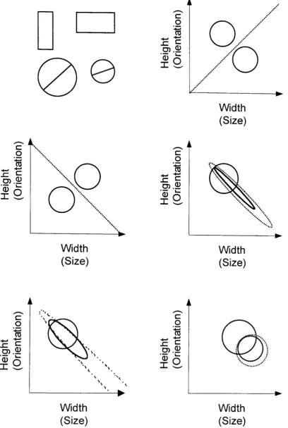
categories and are illustrated in Figure 1 together with examples of the stimuli used

in the experiments. (Because of the very large number of exemplars participants were exposed to, MDS solutions could not be derived for the stimuli, as is normal in

the fitting of the GCM.) Participants were asked to classify rectangles that could vary

in height and width. These dimensions have been shown to be integral (e.g., Garner,

1974; Wiener-Erlich, 1978). Different participants classified circles that could vary in size, with diameters that could vary in orientation. These dimensions have been

found to be separable (e.g., Garner & Felfoldy, 1970; Shepard, 1964).

The category structures for the first two data sets involved two categories

with identical covariance matrices. The variance elements were all identical and the

co-variance elements were all zero, thus the optimal decision bound is linear.

Participants were given a large number of trials. The models were fit to single

participant data. The OEM provided the best fit for 3 participants. The GCM

provided the best fit for 1 participant. The remaining 8 participants' data were best fit by the decision bound model (the general linear classifier), although only slightly

better than the OEM.

The next three data sets also involved two normally distributed categories,

but with unequal co-variance matrices. The optimal decision bounds will therefore

-

o

ro

+-' +-'

..c c:

0> .ID . -

L-IDO

-

ro

..c c:

0> .ID . -

L-IDO

I _

'. _".

'.

". ".

'.

".

··0···,·,·,·,·0

".

_'.

".

-

ro

..c c:

0> .ID . -

L-IDO

-

ro

..c c:

0> .ID ' -

L-IDO

ro

..c c: O>.~

. -

L-IDO

.

Chapter 1 Introduction

O

..

..

.'

... .

..

..

..

.'

..

..

.'

..

co····

: } ... / Width (Size)

..

Figure 1. The stimuli and the five category structures used by Ashby & Maddox

(1992). The top left panel shows two examples of rectangle stimuli and two

examples of the circular stimuli. The remaining panels show the contours of equal

likelihood (solid lines) and optimal decision bounds (dashed lines) for five category

structures used. For the circular stimuli the labels height and width should be

the 24 participants tested exceeded the maximum accuracy possible predicted from a

linear decision bound. Most participants failed to reach the level of performance that

would be predicted if they were perfectly using the optimal quadratic decision

bound. The decision bound model, the DEM and the GCM were applied to data from

the first and last training sessions. For the first training session the decision bound

model (the general quadratic classifier) best fit data from 16 participants, the DEM

best fit in 4 participants, and the GCM best fit in the remaining 4 participants. For

data from the last training session the decision bound model best fit the data from 16 participants, the DEM from 5 participants and the GCM from the remaining 3

participants.

So, modeling individual participant data from participants tested with

normally distributed categories, the GCM was outperformed by the DEM, which in turn was out performed by the relevant decision bound model. Maddox and Ashby (1993) also compared the GCM, the D EM and the decision bound model's fit of data

when participants categorized examples from non-normally distributed categories

using Nosofsky's (1986; 1989) data. The stimuli are the same as the circles with

diameters as described before, except the bottom half of the stimulus is missing. The

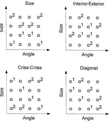
category structure used for these data sets is shown in Figures 2 and 3.

The first data set with non-normally distributed categories (Nosofsky, 1986)

consists of data from two participants who participated in a large number of identification trials for the 16 possible exemplars, so that a MDS solution of the

psychological space representation could be calculated for each participant for the data set. Each participant then took part in four categorization sessions. Each session

began with a training phase, where participants were presented with repeated

Chapter 1 Introduction

Size Interior-Exterior

0

2

2

2

<L>

0 0

2

2

1

1

2

.N N

(j)

0

1

1

C/)

0

2

0 0 ₀

1

1

0

1

1

2

Angle _Angle

Criss-Cross _Diagonal

0

1

2

2

1

2

<L> _{0 0}

1

0 0 <L> 0

1

2

.N _.!:::!

C/)

0

1

C/)

0

1

2

0 0 0 0 0

0

2

2

1

1

2

Angle Angle

Figure 2. The four category structures used by Nosofsky (1986). The circles

correspond to exemplars. Numbered circles are training exemplars, and the

numbers correspond to the category assignment. The remaining exemplars were

Size _Angle

0 0

2

2

Q)

0 0 0

2

2

1

2

N _.N 0

(j)

0

1

1

(j)

0 _{0 0}

1

2

0

1

1

1

2

Angle _Angle

Criss-Cross _Diagonal

0

1

2

2

2

2

Q)

0 0

1

2

1

N _.~

(j)

0

1

(j)

0

2

1

0 0 0 0 0

0

2

2

1

1

1

Angle Angle

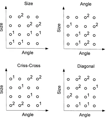
Figure 3. The four category structures used by Nosofsky (1989). The circles

correspond to exemplars. Numbered circles are training exemplars, and the

numbers correspond to the category assignment. The remaining exemplars were

Chapter 1 Introduction 22

In the subsequent transfer task all exemplars were repeatedly, sequentially presented for categorization with feedback given only when a training exemplar was presented.

There were four conditions: two conditions (size and diagonal) where the optimal decision bound is approximately linear and two conditions the optimal decision

bound is non-linear. Maddox and Ashby (1993) fitted the DEM, the GCM and two

decision bound models (the general linear classifier and the general quadratic

classifier). In the two conditions when the best fitting decision bound was

approximately linear there was little difference between the fits of the two exemplar and the two decision bound models. For the conditions where the best fitting

decision bound is non-linear the general quadratic classifier fitted the data

substantially better than the two exemplar models. Ashby and Lee (1992) fitted the optimal decision bound model, and although it did perform better than the GCM it

performed more poorly than the general quadratic classifier, suggesting participants

used a non-optimal classification strategy.

The second data set from non-normally distributed categories (Nosofsky,

1989) differs from the above set in four ways. First, a much larger number of

participants was run. Separate participants were used to derive the MDS solution.

The two dimensional MDS solutions looked much like the arrangement of the

stimuli in physical space shown in (Figure 3). Four new sets of participants took part

in one condition of the categorization stage of the experiment, each set in a different

condition. Second, data was averaged across participants, a procedure which

disadvantages the decision bound models (Maddox, 1999). Third, participants were

given a smaller amount of training before the transfer phase. Finally, one of the

conditions where the best fitting decision bound was non-linear was replaced with a

As a test of the attention-optimization hypothesis (N osofsky, 1986) three

versions of the GCM were fitted to this data set (see also Nosofsky, 1987; Nosofsky, 1989; Nosofsky, 1991). The idea is that selective attention on dimensions in the

psychological space will operate to optimize categorization performance. One of the

versions of the GCM fitted is unconstrained, as described above. The other two

versions are constrained in some way. The equal attention GCM assumes that the

values of Wi in Equation 3 are equal for all

g

assumes that the values of

fu

k

could not be rejected for any of the categorization conditions. The equal attention

GCM fitted the data significantly worse in all four conditions. Some critical transfer stimuli were designed so changes in the relative weighting of the dimensions would

change their probability of assignment to a given category. Observation showed that

the equal attention GCM failed to account for the probability, but the unconstrained GCM did. These results support the idea that the attention weightings for the

dimensions was different in the identification and categorization tasks. The equal

bias GCM fitted the data almost as well as the unconstrained GCM, suggesting that

these results could not be explained by response bias. Lamberts and Chong (1999)

provide further evidence that this phenomena is indeed an attention shift, by showing

that categorization performance changes as a result of verbal instructions directing

attention to particular stimulus dimensions.

The importance of attention shifts may seem problematic for parametric

models, given that they do not incorporate attentional parameters to modify the

perceptual space. However, even without assuming that the perceptual space is

n10dified across the four conditions, decision bound models can account for the

Chapter 1 Introduction 24 and two decision bound models (the general linear classifier and the general

quadratic classifier). The GCM provided the best fit in two conditions (criss-cross

and diagonal), and the general linear classifier provided the best fit in the other two conditions (size and angle). It should be noted that the difference between the

goodness of fits is very small. Further, the GCM fits the averaged participant data

better than the single participant data. That the general linear classifier better fits the two conditions where only one dimension is needed to make the categorization than

the GCM suggests that shifts in decision bounds may be more important than shifts in selective attention. Certainly though, the parametric model is able to account for the "attention shift" phenomena better than the exemplar model.

To summarize the results from data sets from non-normally distributed categories, when modeling individual participants' data after extensive training the

decision bound models provided excellent accounts of the data. However when

modeling data collapsed across participants after a shorter period of training the

difference between the fits of exemplar and decision bound models was smaller. Overall we have seen that exemplar models like the GCM and parametric decision

bound models are able to provide a very good account of empirical data. Decision

bound models outperformed the GCM when category structures were normally

distributed. However with non-normally distributed categories where a smaller

number of exemplars were used, the both models performed about equally.

The Relationship between Exemplar and Parametric Models of Classification

Exemplar and parametric or distributional models can be though of as lying

at opposite ends of a continuum of finite mixture models, where the number of

Rosseel, 1996). Also contained in this continuum are back propagation networks

with sigmoidal activation functions (Rumelhart, Hinton, & Williams, 1986) and

radial basis functions (Moody & Darken, 1989). With small numbers of hidden units (and hence small numbers of free parameters in relation to the size of the data to be

modeled), neural networks are analogous to distributional models, because they can

only learn data with a particular distributional structure. But if the number of hidden

units is large in relation to the amount of data to be learned, then the neural network

becomes analogous to an exemplar model, in that any data set can be modeled,

whatever its structure, simply learning each piece of data (each example) by rote.

The relationship between exemplar and parametric models can be described

formally using Rosseel' s (1998) mixture model of category representation. The

model makes three assumptions. First, following GRT, it is assumed that the

presentation of the same stimulus does not always lead to the same perceptual effect.

The perception of a stimulus is represented as a random vector in multidimensional

psychological space

(19)

where ~!l 12 is a random vector with zero mean representing perceptual noise. ~!l 12 is

multivariate normal with zero mean and co-variance matrix ~!l12. Normally the noise

is assumed to be stimulus invariant and is adequately described by ~.

Second, the probability density function for the whole set of exemplars for all

K categories is modeled as a finite mixture distribution (McLachlan & Basford,

1988; Titterington, 1984): J

p(x)

=

j=l

Chapter 1 Introduction 26 denotes the mixture proportions and satisfy the constraint

J

L

=

j=i (21 )

and I2(?5,

I

lli

Third, this probability density function is shared by each of the K categories. Category

i4

unconditional mixture distribution I2(~).

J

p(xIC

=

LPUlk)p(xlJ)

j=i

where

PG.I

The category representation of the finite mixture model contains the category

representations of exemplar and decision bound models (Ashby & Alfonso-Reese, 1995; Rosseel, 1996). The category representation of the Gaussian GRT is

equivalent to a finite mixture model with one multivariate normal mixture

component. Rosseel (1998) has shown that the category representation of the GeM

using a Gaussian similarity function and a Euclidean distance metric is equivalent to

a finite mixture model with multivariate normal mixture components for each

category exemplar. Further, Rosseel showed that the category representation of the

GCM using an exponential similarity function and a city block distance metric is

equivalent to a finite mixture model with multivariate Laplacian mixture components

for each category exemplar. Thus by altering the number of mixture components,

L

the mixture model can take on the representation assumptions of the GCM (when

I

equals the total number of exemplars across all categories), or Gaussian GRT (when

I

Conclusions

prototype theories of categorization has been presented. The two current accounts of

categorization - exemplar theories and parametric or distributional theories - have

been described in detail. The relationship between various instantiations of each

theory have been described. Empirical evidence collected with the intent of discriminating between these two accounts has been presented. However, it was

concluded that exemplar and distributional approaches both provided good accounts

of the data. Finally the relationship between exemplar and distributional views was formalized using a finite mixture model framework.

Summary of Remaining Chapters

The experiments presented in Chapter 2 of this thesis investigate

generalization to novel items between two categories that differ in variability. It is shown that exemplar and parametric accounts make qualitatively different

predictions for the pattern of generalization. Thus the experiments are designed to

discriminate between the use of exemplar based representations and distributional representations.

The experiments in Chapter 3 of this thesis challenge the assumption that participants have access to the absolute location of stimuli in physical space, an

assumption common to both exemplar and parametric models of categorization. The

experiments were motivated by evidence from absolute identification and magnitude

estimation paradigms, which demonstrates that participants typically have poor

access to absolute magnitude information. Instead participants rely upon

comparisons with recent stimuli, as evident from the strong effect of preceding

material demonstrated in these paradigms. Here specific sequence effects are

examined in categorization - effects that are not predicted by the use of absolute