C
ANP
ERFORMANCE OFI
NDIGENOUSF
ACTORSI
NFLUENCEG
ROWTH ANDG
LOBALISATION?
Kui-Wai Li, Iris A.J. Pang and Michael C.M. Ng
CSGR Working Paper No. 215/07
Can Performance of Indigenous Factors Influence Growth and
Globalisation?
Kui-Wai Li, Iris A.J. Pang and Michael C.M. Ng CSGR Working Paper 215/07
January 2007
Abstract:
This paper employs a total of thirty four openness factors and indigenous factors to construct two
indicators for 62 world economies for the period 1998-2002. While most globalization studies
concentrated on openness factors, regression estimates and simulation studies show that sound
performance in indigenous factors are crucial to an economy’s growth and globalization.
Empirical evidence shows that an optimal performance in indigenous factors can be identified,
and that successful globalized economies are equipped with strong performance in their
indigenous factors.
Keywords:
Globalization, indigenous factors, openness, world economies
Acknowledgements:
We would like to thank Barbara Stallings, Neantro Saavedra-Rivano, Gianluca F. Grimalda, Peter
J. Newell, participants in the APEC Study Center Consortium annual meeting in Ho Chi Ming
City, Vietnam, in May 2006, and two anonymous referees for their comments on the earlier
version of the paper. We are grateful to the funding support from the Faculty of Business, City
University of Hong Kong. The authors are solely responsible for the remaining errors.
Contact Details:
Kui-Wai Li
Department of Economics and Finance, City University of Hong Kong
Tat Chee Avenue, Hong Kong.
CAN PERFORMANCE OF INDIGENOUS FACTORS INFLUENCE GROWTH AND GLOBALIZATION?
I Introduction
Studies on globalization show that factors that determine an economy’s performance in
globalization included trade and income, inequality and poverty, distortion in the factor
market and child labor (Subramanian and Wei 2003; Winters 2002; Deardorff and Stern
2002; Bhagwati 2002; 2004; Aisbett 2005; Frankel 2000; Falvery and Kreickemeier 2005
and Edmonds and Pavcnik 2002). While most pro-globalization advocates (for example,
Feldstein 2000) examined the impact of external or openness factors, anti-globalization
advocates focused on economic sectors that have lost out in the process of globalization
(Wallach and Woodall 2004; Stiglitz 2002). Fischer (2003) noted that globalization is
much more than an economic phenomenon and has non-economic consequences.
Globalization indices have popularly been constructed to rank different world
economies using either a non-parametric approach as in Kearney (2005) or the principal
component analysis as in Andersen and Herbertsson (2005), Heshmati (2006) and
Derher (2006). One commonality in these index construction is the employment of a
number of external economic or openness factors, typically trade and foreign direct
investment, that are grouped into several categories. Only a few domestic or indigenous
factors are included in the calculation of a single globalization index.
Although the performance of the external economy is usually seen from such
openness factors as the level of international trade, capital inflow and the number of
global community, however, depends also on how the domestic sector performed. While
a more matured capital market, for example, will facilitate a greater capital flow, a more
transparent, corruption-free investment environment, for example, could attract more
foreign direct investment. Indigenous factors in an economy can complement the
successful performance of economic openness.
This paper distinguishes indigenous factors from the openness factors. Using
available data from 62 world economies for the period 1998-2002, two separate indices
are constructed for openness factors and indigenous factors. Regression analysis is
conducted to show how the two types of factors can impact on economic growth. To show
the importance of indigenous factors and how they can exert independent influence on
growth and performance in globalization, regression analysis is used to find the optimal
level of performance in an economy’s indigenous factors. Lastly, the 62 world economies
are mapped according to their performance in the openness factors and indigenous
factors. The result shows that economies will have to achieve a certain level in their
performance of the indigenous factors before they can take advantage of economic
openness.
Section II uses an improved method to work out the two indices for the openness
factors and indigenous factors, and the ranking of the 62 world economies. Section III
gives the regression estimates, while section IV compiles an optimal level of performance
in an economy’s indigenous factors and a simulation study is conducted to show how the
62 world economies performed in the two types of factors. Section V concludes the
II The Two Indicators
In constructing the globalization index, Kearney (2005) has grouped openness factors
into four categories of economic integration, technological connectivity, personal contacts
and international engagement. We follow this classification but improve the list of
openness factors by incorporating the pattern of external trade of an economy in two
aspects. Namely, while an economy’s inter-industry trade is traditionally based on
comparative advantage, an economy’s intra-industry trade reflects its pattern of foreign
direct investment and availability of technology. Trade statistics are post-trade data that
reflect the outcome of trade policies. The performance of inter-industry trade can be seen
from an economy’s revealed comparative advantage (RCA) index (Balassa 1965; 1977;
1979; 1986).1 When the value of ,
it g
RCA exceeds unity, economy i is said to have a
revealed comparative advantage in good g at time t. The total number of export industries
of individual economies with revealed comparative advantage greater than unity are
selected and normalized (NRCA) to form an indicator for the economy’s inter-industry
trade performance (TRCAit).2
In intra-industry trade, economies export and import the same good or service in a
given period. Intra-industry trade reflects more on the varieties of goods the economy
enjoys due to industrial diversity and technological advancement than simply on trade
1 The RCA index can be calculated as:
(
(
)
(
)
)
,
i t g i g w g i w t
R C A = X X X X , where Xig
denotes economy i’s export of commodity g, Xwg is world export of commodity g, Xi is economy i’s total export and Xw is total world exports, where i=1,…,N, t=1,…,T and g=1,…,G.
2
(
{
}
)
flows based on comparative advantages. The extent of global economic integration
through market structure and industry pattern can be seen from the level of intra-industry
trade that also reflected the outcome of investment by multinational enterprises. The
intra-industry trade index (IIT) can be calculated as:
(
)
(
)
, , , , , , , ,
1 1
1 *100 1 *100
j j
n n
it ij g ij g ij g ij g ij g ij g ij g ij g i
j g g j g g
t
IIT X M X M MAX X M X M
= =
⎛ ⎧⎪⎡ ⎤ ⎫⎪ ⎧⎪ ⎛⎡ ⎤ ⎞⎫⎪⎞
⎜ ⎟
=⎜ ⎨⎢ − − + ⎥ ⎬ ⎨ ⎜⎜⎢ − − + ⎥ ⎟⎟⎬⎟
⎪⎣ ⎦ ⎪ ⎪ ⎣ ⎦ ⎪
⎩ ⎭ ⎩ ⎝ ⎠⎭
⎝
∑ ∑
∑
∑ ∑
∑
⎠,
(1)
where Xij,g is the export value of good g from country i to country j,Mij,g is the import value
of good g to country i from country j, and nj= total number of economy i’s trading
partners. Equation (1) shows the weighted average of individual industry indices, where
the weights are the shares of industries in total trade.3
The data used in the construction of the Openness Factors Indicator (OFI) come
from 17 external economic openness factors grouped under six categories. There are few
exceptions. For example, Hong Kong has little international engagement in government
transfer and financial contribution to the United Nations Security Council missions.
Although the intention is to obtain as large a number of factors as possible, the data are
more constrained in the construction of the Indigenous Factors Indicator (IFI). Data on a
total of 17 indigenous factors are classified into three broad categories. While the first
category of institutional establishment is considered as proxy measures for civility,
security and protection of individuals, the other two categories provide indicators on the
3 The intra-industry trade index is compiled using the UN Comtrade Database, SITC Rev.3 (UN Comtrade,
quality of life. Table 1 summarizes the categories of openness factors and indigenous
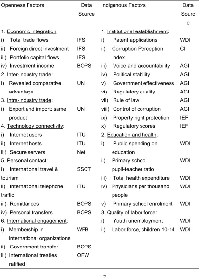
[image:7.595.85.490.188.753.2]factors and the data sources.
Table 1 The Classification of Openness Factors and Indigenous Factors
Openness Factors Data
Source
Indigenous Factors Data
Sourc e 1. Economic integration:
i) Total trade flows
ii) Foreign direct investment iii) Portfolio capital flows iv) Investment income 2. Inter-industry trade: i) Revealed comparative
advantage
3. Intra-industry trade: i) Export and import: same
product
4. Technology connectivity: i) Internet users
ii) Internet hosts iii) Secure servers 5. Personal contact: i) International travel & tourism
ii) International telephone traffic
iii) Remittances iv) Personal transfers
6. International engagement: i) Membership in
international organizations ii) Government transfer iii) International treaties
ratified IFS IFS IFS BOPS UN UN ITU ITU Net SSCT ITU BOPS BOPS WFB BOPS OFW
1. Institutional establishment: i) Patent applications ii) Corruption Perception
Index
iii) Voice and accountability iv) Political stability
v) Government effectiveness vi) Regulatory quality
vii) Rule of law
viii) Control of corruption ix) Property right protection x) Regulatory scores 2. Education and health: i) Public spending on
education
ii) Primary school pupil-teacher ratio
iii) Total health expenditure iv) Physicians per thousand
people
v) Primary school enrolment 3. Quality of labor force: i) Youth unemployment ii) Labor force, children 10-14
iv) Personnel and financial contribution to United Nations Security Council missions
UNDPI
Notes:
IFS = International Financial Statistics, International Monetary Fund; BOPS = Balance of Payment Statistics, United Nations;
UN = United Nations Comtrade, United Nations;
ITU = International Telecommunication Union Database, International Telecommunication Union;
Net = Netcraft Secure, International Telecommunication Union;
SSCT = Server Surveys Compendium of Tourism Statistics, World Tourism Organization;
WFB = The World Factbook, Central Intelligence Agency; OFW = Official websites of selected basket of treaties;
UNDPI = United National Development Program Indicators, United Nations; WDI = World Development Indicators, World Bank;
CI = Corruption Index 1996-2002, Transparency House;
AGI = Aggregating Governance Indicators 1996-2004, World Bank; IEF = Index of Economic Freedom, Heritage Foundation.
A total of 62 world economies have data on all or most of the openness factors and
indigenous factors. Data for the three years in 1998-2001 are complete, while some 2002
data are either provisional or unavailable. Both the openness and indigenous factors are
normalized on a yearly basis, as suggested in Lockwood (2004), before they are used to
construct the OFI and IFI.4
We apply the principal component analysis (PCA) to the indicators yearly. There
4 The normalization formulas for the high and low value variables that represent a higher degree of
openness (in OFI) and a more advanced indigenous environment (in IFI), respectively, are:
( i N N N )t
it v v v v v v v
V = −min{ 1,..., }/{max( 1,..., )−min( 1,..., )} , and
(
N i N N)
tit v v v v v v v
are several advantages in using the PCA method. Firstly, since these indicators are likely
to be correlated, the PCA reduces these indicators to fewer variables that capture the
maximum variation. Secondly, the PCA method can commensurate on the different
measurement units of these indicators. Most importantly, the PCA method gives
data-driven weights to the indicators that form the ultimate principal components. The
principal components are extracted from the correlation matrix of the variables, in a way
that they accounted for the highest percentage of variation. The PCA is applied to each
individual year instead of applying one PCA to the whole sample period. This has the
advantage of incorporating various changes in the sample period, and can eliminate the
impact of a sudden change in any particular year that could affect other sample years.
We adopt a latent variable model and postulate that the indicator is linearly
dependent on a set of observable factors (V) and an error term (Rencher 2002). The
principal components (PCs) are computed from the following procedure:
1 11 1 1
2 21 1 2
1 1
L L L
PC V V
PC V V
PC V V
α
α
α
α
α
α
Ψ Ψ
Ψ Ψ
Ψ Ψ
= + +
⎧
⎪ = + +
⎪ ⎨ ⎪
⎪ = + +
⎩
L L M
L
, (2)
where
α α
11, 12,L,α
1Ψare elements of eigenvectorα
1={
α
11,L,α
1Ψ}
, and there are atotal of L eigenvectors, which are determined by the data. A total of L principal
components are computed using successive eigenvectors elements, α1, α2,…,αL,
corresponding to the largest L eigenvalues,
λ
1 >λ
2 >L>λ
L, of the factor correlationvariance becomes our OFI, which is then normalized or scaled.5 The scaled OFI will take
a value of unity when an economy has the best performance in its external environment.
The same procedures are applied to the construction of the IFI.
In constructing the two indicators, the missing values are replaced by their nearby
means.6 Different weightings are generated from a corresponding principal component
analysis for economies that an entire series of a factor is missing. The methodology is an
improvement on Anderson and Herbertsson (2005) and Dreher (2006). Andersen and
Herbertsson (2005) used a single principal component analysis for all the data in their
sample period of 1979 to 2000, and they provided rankings of economies according to
the factor scores for each year generated by pooling the years over the sample period.
However, taking Lockwood’s (2004) suggestion on normalization, the problem of the
methodology in Anderson and Herbertsson (2005) is that the change in the ranking of
one economy in a specific year would change the rankings of other economies over the
whole sample period. Dreher (2006) used weightings of principal component analysis
from year 2000 for the calculation of indices for each single year from 1970 to 2000. The
principal component analysis is meant to give weightings that maximize the variance of
the indices, but if weightings generated in 2000 are used for the indicator of all preceding
years, the maximum variance effect is lost and the principal component analysis would
seem meaningless.
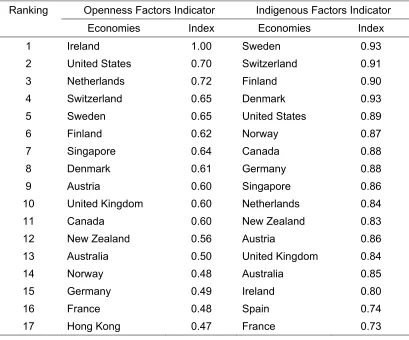
Table 2 gives the five-year (1998-2002) average of the OFI and IFI indicators. The
5
(
{
}
{
}
{
}
)
m in m ax m in
it i i i i
t
S ca led O F I = O F I − O F I O F I − O F I
6 In the Openness Factors Indicators, the maximum number of missing economies in the 1998-2002 sample
ranking based on the five-year average shows that the top 10 economies in the two
indices are mainly advanced economies in North America and Western Europe. Most of
the remaining European Union economies are included when the scores are extended to
the top 20. Singapore and Hong Kong are the only two Asian economies in the top 20 of
both indicators. We observe that an economy can vary between the two indicators. For
example, Japan ranked 18th in the IFI, but ranked 26th in the OFI, while Indonesia ranked
44th and 55th in OFI and IFI, respectively. Economically weaker economies tend to rank
lower in the two indicators. Effectively, economies that ranked below 30th are all
[image:11.595.87.496.390.730.2]developing economies.
Table 2 Openness Factors and Indigenous Factors Indicators (62 World Economies, 1998-2002 Average)
Openness Factors Indicator Indigenous Factors Indicator Ranking
53 54 55 56 57 58 59 60 61 62 Nigeria Egypt Kenya Morocco Pakistan Sri Lanka Uganda Saudi Arabic Iran Bangladesh 0.07 0.07 0.06 0.05 0.05 0.04 0.04 0.03 0.03 0.01 Iran China Indonesia Ukraine Senegal Kenya Pakistan Uganda Bangladesh Nigeria 0.21 0.22 0.16 0.21 0.19 0.13 0.12 0.10 0.03 0.00
III Regression Estimates
We make use of the two indicators and postulate the hypothesis that economies with
strong performance in indigenous factors do enjoy a higher rate of per capita GDP growth
at different level of economic openness. We first divide the IFI into k portions using
percentiles, shown in Equation (3), with N being the number of economies.
{ }
(
(
)
)
{
}
{
(
(
(
)
)
)
(
(
)
)
}
(
)
(
)
(
)
(
(
)
)
{
}
min , , 100 % , 100 1 % , , 2 100 %
, , 1 100 1 % , , 100 % .
th
th th
t
i t t
th th
t
IFI IFI k N IFI k N IFI k N IFI
k k N IFI k k N IFI
= × + × × ×
− × + × × ×
L L
L L
(3)
For example, we can divide the IFI of year t into three portions, so k = 3, with 33.33
percent of the economies in each portion. The first portion is made up of the minimum IFI
in year t to the 33rd IFI in year t. We then assign a dummy variable,Dκ, where κ=1,…, k,
of unity if IFIit falls into the κth portion, otherwise it takes a value of zero. Since the IFI is a
measure of the indigenous environment of an economy, and the higher the IFI value an
economy has, the better is its indigenous environment. Namely, an economy with
1
= κ
D has a better indigenous environment than an economy with Dκ−1 =1.
We use the following model to examine how indigenous factors can affect the
outcome of openness on growth:
, *
ln *
ln ln
lnyit =
α
+β
1 OFIit +β
2 OFIit D2,it +L+β
k OFIit Dk,it +ε
it (4)where yit is the real GDP per capita deflated by the purchasing power parity of economy i
at time t. For economy i who has the dummyDκ =1, the regression equation become:
, ln
ln
ln yit =
α
+β
1 OFIit +β
κ OFIit +ε
it or (5)(
)
ln .ln yit =
α
+β
1+β
κ OFIit +ε
itFor another economy j which has the dummy Dκ−c =1, for any c > 0. In other words, when economy j’s indigenous environment is not as good as economy i’s, the regression
equation become:
, ln
ln
lnyjt =
α
+β
1 OFIit+β
κ−c OFIjt+ε
jt or (6)(
)
ln .lnyjt =
α
+β
1+β
κ−c OFIjt+ε
jtIf a higher performance in indigenous factors brings a higher marginal effect of
generalizing all the k dummy variables, and if a better indigenous environment has a
positive impact of openness on growth, we expect to see β1 <β1 +β2 <β1 +β3 < … <β1 +βk,
suggesting that a strong performance in an economy’s indigenous factors enables an
economy to benefit more from openness. We conducted two Wald tests to show the
significance of the coefficient estimates. The first Wald test is to see if a low performance
in the indigenous factors constrained economic growth. We propose an alternative
hypothesis with
β
1< 0, which implies that if an economy has an extremely weakperformance in its indigenous factors (reflected in the IFI value falling into the first
partition of the indicator), openness would bring negative effects on economic growth,
namely: . 0 : 0 : 1 1 1 1 < =
β
β
Ha Ho (7)The second Wald test shows that an economy’s IFI can significantly affect the marginal
effect of an economy’s openness on its real per capita GDP growth rate:
. , , 3 : . , , 2 0 : 1 1 1 2 1 2 k for Ha k for Ho L L = + < + = = +
−
β
β
κ
β
β
κ
β
β
κ κ κ (8)The alternative hypothesis, 2
Ha , states that economies that have a better performance in
their indigenous factors should benefit more from openness.
We applied the within-GLS method to estimate Equation (4), but the emergence of
the singular matrix problem due probably to the short sample period led us instead to use
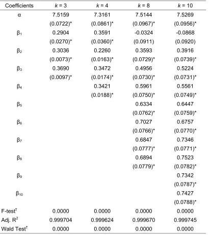
Equation (4) is estimated with k = 3, 4, 8 and10. Table 3 shows the empirical estimation
[image:16.595.85.495.219.680.2]of the pooled-GLS results for the 62 countries for the sample period of 1998-2002.
Table 3 Pooled-GLS Estimates of 62 World Economies, 1998-2002
Coefficients k = 3 k = 4 k = 8 k = 10
α 7.5159
(0.0722)* 7.3161 (0.0861)* 7.5144 (0.0967)* 7.5269 (0.0956)*
β1 0.2904
(0.0270)* 0.3591 (0.0360)* -0.0324 (0.0911) -0.0868 (0.0920)
β2 0.3036
(0.0073)* 0.2260 (0.0163)* 0.3593 (0.0729)* 0.3916 (0.0739)*
β3 0.3690
(0.0097)* 0.3472 (0.0174)* 0.4956 (0.0730)* 0.5224 (0.0731)*
β4 0.3421
(0.0188)*
0.5961 (0.0750)*
0.5561 (0.0749)*
β5 0.6334
(0.0762)*
0.6447 (0.0759)*
β6 0.7027
(0.0766)*
0.6757 (0.0770)*
β7 0.6847
(0.0777)*
0.7346 (0.0771)*
β8 0.6894
(0.0779)*
0.7523 (0.0782)*
β9 0.7342
(0.0787)*
β10 0.7427
(0.0788)* F-test†
Adj. R2 Wald Test†
0.0000 0.999704 0.0000 0.0000 0.999624 0.0000 0.0000 0.999670 0.0000 0.0000 0.999745 0.0000 Notes: Figures in parentheses are standard errors.
All estimates with k = 3 and k = 4 in Table 3 are significant at 1 percent level. In
these two cases, the estimate for β1 is not negative, but is significantly different from zero,
suggesting that a low performance in indigenous factors does not adversely affect the
effect of globalization on economic growth, though this may be due to the small size of k.
When the size of k is small, the marginal effect of indigenous factors on globalization and
economic growth may not be obvious. The F-tests reject the null hypothesis of Equation
(4), and suggests that as economies improve the performance of their indigenous factors,
the marginal effect of globalization on growth increases.
For estimates with k = 8 and k = 10, and with the exception of the insignificant
estimate for β1, all the estimates are significance at 1 percent level. For these estimated
values of k, the estimate of β1 is negative, which means that growth in an economy with
low performance in indigenous factors can adversely be affected by globalization. Similar
to the results of k = 3 and k = 4, the F-tests reject the null hypothesis. This confirms that
improvement in the performance of indigenous factors in an economy can improve the
marginal effect of globalization on growth.
IV Optimal Performance in Indigenous Factors
This section uses a simulation method to work out the optimal performance in the
indigenous factors in order to achieve a maximum gain in economic growth. From the
in IFI to see if there is diminishing returns in economic openness. Hypothetical economies
are compared in order to see how an economy performs in growth and globalization
given a different level of performance in indigenous factors. We established two
hypotheses. First, given two externally homogeneous economies (namely, economies
with same performance in the OFI), heterogeneity in the performance of IFI will lead to
differences in economic growth and development. Secondly, given homogeneity in the
performance of IFI among different economies, those economies with a better
performance in OFI will result in higher economic growth.
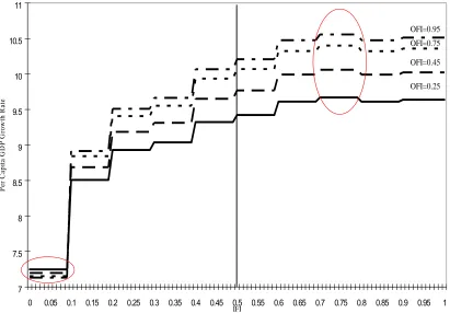
We make use of the empirical result with k = 10 in Table 3 to simulate the growth of
GDP per capita for a total of 100 hypothetical economies with an incremental change of
0.01 in the IFI that ranged from zero to one. We set different values of the OFI that are
either below or above the median value. A simulated series of per capita GDP figures are
generated from the empirical results with k = 10 in Table 3.7 The simulated per capita
GDP growth rates are plotted against the IFI, and a step function is presented separately
for the four values of OFI (at 0.25, 0.45. 0.75 and 0.95) as shown in Figure 1.
7 For example, when OFI = 0.25, and with 1 , 3it =
D (namely, the range of IFI is between 0.2 and 0.3, and other dummies take a zero value), the simulated GDP per capita growth is 8.92904 (i.e. 7.52687 +
7 7.5 8 8.5 9 9.5 10 10.5 11
0 0.05 0.1 0.15 0.2 0.25 0.3 0.35 0.4 0.45 0.5 0.55 0.6 0.65 0.7 0.75 0.8 0.85 0.9 0.95 1
IFI
P
er
C
ap
ita
G
D
P
G
ro
w
th
R
ate
OFI=0.95
[image:19.595.101.512.121.407.2]OFI=0.25 OFI=0.45 OFI=0.75
Figure 1 Effect of Economic Openness on Growth
The first observation in Figure 1 is that economies with a higher performance in
openness (with higher OFI) produced a higher level of per capita GDP growth at all level
of IFI above 0.1. In economies with IFI below the median, a higher performance in OFI
always produced a higher economic growth measured in GDP per capita, except when
IFI is below 0.1. The second observation is that, when the IFI is above median, economic
growth kept rising regardless of the performance in the OFI until an economy’s IFI
reached the range of 0.7 and 0.8, beyond which the growth rate of GDP per capita
economies will reach their highest possible growth rates given their OFI.
When the value of OFI lies between 0 and 1, the marginal contribution of IFI to the
per capita GDP growth of an economy is positive if the value of IFI lies between 0 and the
optimal level. When the value of IFI is above its optimal level, the marginal contribution of
IFI to an economy’s GDP per capita growth is negative.8 In short, if an economy has an
IFI value below 0.1, a lower value of OFI actually produces a higher per capital GDP
growth. So long as the value of IFI lies above 0.1, the marginal contribution by the
different level of OFI to per capita GDP growth is positive. On the contrary, when IFI lies
between 0 and 0.1, the marginal contribution of OFI to per capita GDP growth is
negative.9
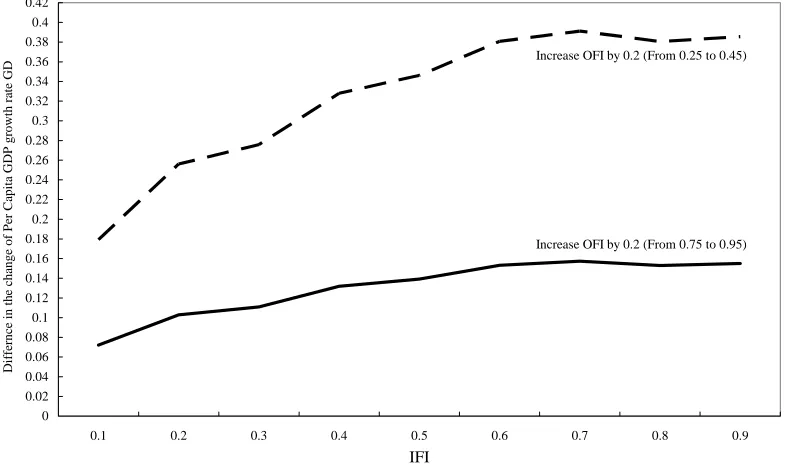
The analysis can be extended to examine the marginal effect of both OFI and IFI. By
plotting the change in the per capita GDP growth rate against the IFI at different level of
the OFI, Figure 2 shows that, at different level of IFI, a higher OFI can lead to a larger
change ingrowth rate of per capita GDP.10 However, as shown in Figure 3, the marginal
effect of IFI on the change in growth rate of per capita GDP at different level of OFI is
increasing at a decreasing rate. Furthermore, Figure 3 shows that when the OFI value is
8 This can also be seen if Equation (4) is modeled as a continuous or differentiable function, where 0< i < 1,
and IFI* represents the optimal value:
0 ln ; 0 ln ; 0 ln ; ; ,
0 * *
< ∂ ∂ > ∂ ∂ > ∂ ∂ = > = < = < < i i
i IFI IFI OFI OFI IFI IFI OFI OFI
OFI OFI Median IFI IFI y IFI y IFI y
9 When the function is a differentiable, the results can be summarized as follows:
0 ln ln ; 0 ln ln ; 0 ln ln 1 . 0 0 5 . 0 1 . 0 1 5 . 0 < ∂ ∂ > ∂ ∂ > ∂ ∂ < < < < <
<IFI IFI OFI IFI
y OFI
y OFI
y
10 The marginal effect can be summarized as follows when a differentiable equation is used:
below median, the marginal contribution of economic openness towards the economics
growth is larger than that when OFI is above median.11
-0.2 0 0.2 0.4 0.6 0.8 1 1.2 1.4 1.6 1.8 2
0.1 0.2 0.3 0.4 0.5 0.6 0.7 0.8 0.9
IFI
C
h
ange
in P
er
c
apita GDP
Gr
owth
OFI=0.95
[image:21.595.98.489.184.423.2]OFI=0.25 OFI=0.45 OFI=0.75
Figure 2 Marginal Effect of OFI on Growth
11 The marginal effect can be summarized as follows when a differentiable equation is used:
Median Above Median
Below OFI
Y OFI
Y
∂ ∂ >
∂ ∂
ln ln ln
Figure 3 Effect of a Change in OFI
With the construction of the two indicators that look separately at indigenous factors
and openness factors, the regression and simulation results provided additional evidence
to other studies (for example, Hesmati 2006) that indigenous factors can have
independent influence on growth and openness. Various policy recommendations can
then be suggested from the empirical and simulation analysis. Firstly, a more globalized
economy indicated by the higher performance in economic openness does not always
lead to higher economic growth; for those economies with 0 < IFI < 0.1, they should
improve on the IFI in order to reap additional gain from openness and ultimately
globalization. Secondly, economies whose IFI is above 0.1, but below the optimal range
(0.7 to 0.8), should aim to improve the performance of the indigenous factors, hoping
gradually to reach the optimal level.
A pattern of relationship between economic growth, performance in the openness
0 0.02 0.04 0.06 0.08 0.1 0.12 0.14 0.16 0.18 0.2 0.22 0.24 0.26 0.28 0.3 0.32 0.34 0.36 0.38 0.4 0.42
0.1 0.2 0.3 0.4 0.5 0.6 0.7 0.8 0.9
IFI
Dif
fe
rnce
i
n
th
e cha
nge
of
P
er C
apita
G
D
P
gr
owth ra
te
GD
Increase OFI by 0.2 (From 0.25 to 0.45)
factors and indigenous factors seems to have emerged from the simulation analysis.
Figure 4 argues that once the performance in the indigenous factors has reached a
minimum level, improvement in indigenous factors will lead to a larger per capita GDP
growth rate at every higher level of openness. Thus, at a high level of openness, OFI3 for
[image:23.595.115.482.268.524.2]example, a higher level of per capita GDP growth rate can be achieved.
Figure 4 Relationships between Growth, Openness and Indigenous Factors
To see how the 62 world economies perform in the 1998-2002 period, Table 4 maps
out the sample period average in five different ranges of OFI and IFI. Individual
economies can consider their own positions in the ranking of the two indicators, and
compare their performance with other economies, including the periodic average in the
GDP per capita growth rates. There are seven mainly poor developing economies
(Bangladesh, Indonesia, Kenya, Nigeria, Pakistan, Senegal and Uganda) that have the IFI GDP Growth Rate (%)
OFI1
OFI3
OFI2
OFI3>OFI2>OFI1
lowest rankings in both indicators. On the contrary, those economies that performed
strongly in both OFI and IFI are mainly developed economies (Austria, Denmark, Finland,
Netherlands, Singapore, Sweden, Switzerland, United Kingdom and USA). Most
developed economies have performed stronger in IFI than in OFI. Ireland is the only
economy that has a stronger performance in OFI than in IFI in the sample period.12
The observation from Table 4 is that performance of indigenous factors is the more
relevant constraint in the globalization process of any economy. Most economies that are
strong in the performance of IFI are also strong in the performance of OFI, but not the
reverse. In other words, it would be appropriate for economies to improve their
indigenous conditions and environment before they can gain from openness and
globalization. Economies have to achieve a reasonable level of performance in
indigenous factors before gaining the benefits from openness factors. A good
performance in indigenous factors is essential to openness, growth and development.
There are a number of economies (Argentina, Botswana and so on) that have achieved a
median in IFI, but showed low performance in OFI. The 0.61 to 0.80 range of the IFI
seems to be the critical range, as virtually all industrially advanced economies achieved
an IFI score above 0.61.
Table 4 shows that a number of economies in the second lowest (0.21 – 0.40) range
of IFI experienced a relative high growth rate in the sample period. For example, China
has a growth rate of 6.749 percent and the Russian Federation had 6.381 percent and so
on. This suggested that these economies have to improve their IFI before reaping the
12 Measured in purchasing power parity constant 2000 price, Ireland’s GDP per capita is highest among the
gain from openness and globalization. Among the developing economies, African
economies (e.g. Uganda, Kenya and Senegal) are the weakest performers in both the
OFI and IFI, while the middle-ranking economies are the few Asian (e.g. Thailand and
Malaysia) and Latin American (e.g. Panama and Chile) economies. Other Asian
economies (e.g. India, Indonesia, Philippines and Sri Lanka) performed poorly in both
OFI and IFI. The group of developing economies that have reached the range of 0.61 –
0.80 in the IFI are mostly Eastern European economies (e.g. Hungary, Slovenia and
Czech Republic), which will probably be the next group of countries that would benefit
from globalization. The lesson is that sound performance in the various indigenous
factors will facilitate good performance of openness factors. In short, advancement in the
Table 4 The OFI – IFI Matrix of World Economies, 1998-2002 Average Indigenous Factors Indicator (IFI)
Range 0.00 - 0.20 0.21 - 0.40 0.41 - 0.60 0.61 - 0.80 0.81 - 1.00
0.00 - 0.20 Uganda (4.049) Bangladesh (3.025)* Senegal (2.322) Nigeria (1.575)* Indonesia (1.408) Pakistan (1.398) Kenya (-1.343) China (6.749) Russian Fed. (6.381) Ukraine (5.692) India (3.287) Romania (3.071) Egypt (2.932) Iran (2.786) Sri Lanka (1.928)
Philippines (1.239) Brazil (1.229) S. Africa (1.227) Mexico (1.001) Peru (0.768) Turkey (-0.096) Colombia (-0.807) Venezuela (-3.697) Botswana (8.615) Tunisia (3.198) Thailand (2.911) Chile (1.072) Morocco (0.720) Saudi Arab. (-0.938) Argentina (-5.887)
0.21 - 0.40
Croatia (3.654) Korea (5.957)
Greece (4.207) Slovak Rep. (3.341) Poland (2.981) Malaysia (2.945) Panama (0.661)
Hungary (3.869) Slovenia (3.858) Czech Rep. (3.354) Spain (2.671) Portugal (1.945) Italy (1.590) Japan (0.477) Israel (-0.096) Ope nness F actors Indica to r ( OF I ) 0.41 - 0.60
Hong Kong (3.346)
France (2.201)
0.61 - 0.80
Singapore (4.082)
Sweden (2.500) Finland (2.161) U.K. (2.102) Denmark (1.788) Austria (1.723) Netherlands (1.617) USA (1.455) Switzerland (1.095) 0.81 -
1.00
Ireland (9.737)
V Conclusion
Recent globalization indices ranked the performance of different world economies with
few or without the inclusion of domestic or indigenous factors (Anderson and Herbertsson
2005, Kearney 2005 and Dreher 2006). The empirical results in the paper add to the
globalization debate and the construction of the globalization index by making reference
separately to the relevance and importance of a number of indigenous factors.
In constructing the OFI, this paper takes into account the pattern of trade and
industries by incorporating the inter-industry and intra-industry trade, in addition to the
total trade flows. The number of indigenous factors used in the construction of IFI should
provide a more comprehensive picture on the domestic performance of different
economies. The regression result that indigenous factors are important in promoting an
economy’s growth led to further investigation and analysis on the relationship between
the two types of factors. Given different level of performance in the economy’s openness,
a higher performance in the IFI will produce a higher growth rate. When the performance
of an economy’s indigenous factors is extremely low, it would be more appropriate for
that economy to improve its indigenous factors than to engage in globalization. In short,
performance in the indigenous factors is the more fundamental issue than economic
openness. Before the “optimal” level of indigenous factors performance is reached, the
economy will get better off in per capita GDP as the performance of indigenous factors
improve.
Literature on the gain from globalization points to the importance of a sound
performance in both the openness and indigenous factors, one comes to the conclusion
that sound performance in the indigenous factors is very crucial to economic openness
and globalization. All economies with strong performance in economic openness and
globalization have sound performance in their indigenous factors. For those world
economies that are ranked low in the IFI, appropriate economic policies should be
References
Aisbett, E. (2005) Why are the Critics so Convinced that Globalization is Bad for the Poor?, Working Paper No. 11066, National Bureau of Economic Research.
Andersen, T., and Herbertsson, T. (2005) Quantifying Globalization, Applied Economics, 37, pp. 1089-1098.
Balassa, B. (1965) Traded Liberalization and ‘Revealed’ Comparative Advantage, The Manchester School of Economic and Social Studies, 33, pp. 99-123. Balassa, B. (1977) Revealed’ Comparative Advantage Revisited: An Analysis of
Relative Export Shares of the Industrial Countries, 1953-1971, The Manchester School of Economic and Social Studies, 45, pp. 327-344. Balassa, B. (1979) The Changing Pattern of Comparative Advantage in
Manufactured Goods, Review of Economics and Statistics, 61(2), pp. 259-266.
Balassa, B. (1986) Comparative Advantage in Manufactured Goods: A Reappraisal, Review of Economics and Statistics, 68(2), pp. 315-319. Bhagwati, J. (2002) Free Trade Today, (Princeton: Princeton University Press). Bhagwati, J. (2004) In Defense of Globalization, (New York: Oxford University
Press).
Central Intelligent Agency, (1998-2002) The World Factbook. (Washington D C: Central Intelligent Agency).
Deardorff, A., and Stern, R. (2002) What You Should Know about Globalization and the World Trade Organization, Review of International Economics, 10 (3), pp. 404-423.
Dreher, A. (2006) Does Globalization Affect Growth? Evidence from a New Index of Globalization, Applied Economics (forthcoming).
Edmonds, E., and Pavcnik, N. (2002) Does Globalization Increase Child Labor? Evidence from Vietnam, Working Paper 8760, National Bureau of
Economic Research.
Falvery, R., and Kreickemeier, E. (2005) Globalization and Factor Returns in Competitive Markets, Journal of International Economics, 66, pp. 233-248. Feldstein, M. (2000) Aspects of Global Economic Integration: Outlook for the
Future, Working Paper 7899, National Bureau of Economic Research. Fischer, S. (2003) Globalization and Its Challenge, Ely Lecture, American
Frankel, J. (2000) Globalization of the Economy, Working Paper 7858, National Bureau of Economic Research.
Heritage Foundation, (1998-2002) Index of Economic Freedom, (Washington D C: Heritage Foundation).
Heshmati, A. (2006) Measurement of a Multidimensional Index of Globalization, Global Economy Journal, 6 – 2 Article 1.
International Telecommunication Union, (1998-2002) International Telecommunication Union Database, (Geneva: International Telecommunication Union).
International Telecommunication Union, (1998-2002) Netcraft Secure Server Surveys, (Geneva: International Telecommunication Union).
International Monetary Fund, (1998-2002) International Financial Statistics, (Washington D C: International Monetary Fund).
Kearney, A. (2005) Measuring Globalization: Economic Reversals, Forward Momentum, (Washington D C: Foreign Policy).
Lockwood, B. (2004) How Robust is the Foreign Policy-Kearney Globalisation Index?, The World Economy, 27, pp. 507--523.
Rencher, A. (2002) Methods of Multivariate Analysis, Second Edition, (New York: Wiley-Interscience).
Stiglitz, J. (2002) Globalization and Its Discontent, (London: Allen Lane). Subramanian, A., and Wei, S. (2003) The WTO Promotes Trade, Strongly but
Unevenly, Working Paper 10024, National Bureau of Economic Research. Transparency House, (2003) Corruption Index 1996-2002, (Washington D C:
Transparency House).
United Nations, (1998-2002) Balance of Payments Statistics, (New York: United Nations).
United Nations, (1998-2002) United Nations Development Program Indicators, (New York: United Nations).
United Nations, (1998-2002) United Nations Comtrade, (New York: United Nations).
Wallach, L., and Woodall, P. (2004) Whose Trade Organization, (New York: The New Press).
Winters, L. (2002) Trade Policies for Poverty Alleviation, in Hoekman, B. Mattoo, A. and English, P. (Eds.), Development, Trade and the WTO: A Handbook, (Washington D C: The World Bank).
World Bank).
World Bank, (1998-2002) World Development Indicators, (Washington D C: World Bank).
CSGR Working Paper Series
189/06, January Amrita Dhillon, Javier Garcia-Fronti, Sayantan Ghosal and Marcus Miller Bargaining and Sustainability: The Argentine Debt Swap
190/06 January Marcus Miller, Javier Garcia-Fronti and Lei Zhang
Contractionary devaluation and credit crunch: Analysing Argentina. 191/06 January Wyn Grant
Why It Won’t Be Like This All The Time: the Shift from Duopoly to Oligopoly in Agricultural Trade
192/06 January Michael Keating
Global best practice(s) and electricity sector reform in Uganda 193/06 February Natalie Chen, Paola Conconi and Carlo Perroni
Does migration empower married women? 194/06 February Emanuel Kohlscheen
Why are there serial defaulters? Quasi-experimental evidence from constitutions. 195/06 March Torsten Strulik
Knowledge politics in the field of global finance? The emergence of a cognitive approach in banking supervision
196/06 March Mark Beeson and Hidetaka Yoshimatsu
Asia’s Odd Men Out: Australia, Japan, and the Politics of Regionalism 197/06 March Javier Garcia Fronti and Lei Zhang
Political Instability and the Peso Problem 198/06 March Hidetaka YOSHIMATSU
Collective Action Problems and Regional Integration in ASEAN 199/06 March Eddy Lee and Marco Vivarelli
200/06 April Jan Aart Scholte
Political Parties and Global Democracy 201/06 April Peter Newell
Civil society participation in trade policy-making in Latin America: The Case of the Environmental Movement
202/06 April Marcus Miller and Dania Thomas
Sovereign Debt Restructuring: The Judge, the Vultures and Creditor Rights 203/06 April Fondo Sikod
Globalisation and Rural Development in Africa: The Case of the Chad-Cameroon Oil Pipeline.
204/06 April Gilles Quentel
The Translation of a Crucial Political Speech: G.W.Bush’ State of the Union Address 2003 in Le Monde
205/06 April Paola Robotti
Arbitrage and Short Selling: A Political Economy Approach 206/06 May T.Huw Edwards
Measuring Global and Regional Trade Integration in terms of Concentration of Access 207/06 May Dilip K. Das
Development, Developing Economies and the Doha Round of Multilateral Trade Negotiations
208/06 May Alla Glinchikova
A New Challenge for Civic National Integration: A Perspective from Russia. 209/06 June Celine Tan
210/06 September Richard Higgott
International Political Economy (IPE) and the Demand for Political Philosophy in an Era of Globalisation
211/06 October Peter Waterman
Union Organisations, Social Movements and the Augean Stables of Global Governance 212/06 October Peter Waterman and Kyle Pope
The Bamako Appeal of Samir Amin: A Post-Modern Janus? 213/06 October Marcus Miller, Javier García-Fronti and Lei Zhang
Supply Shocks and Currency Crises: The Policy Dilemma Reconsidered 214/06 December Gianluca Grimalda
Which Relation between Globalisation and Individual Propensity to Co-Operate? Some Preliminary Results from an Experimental Investigation
215/07 January Kui-Wai Li, Iris A.J. Pang and Michael C.M. Ng
Can Performance of Indigenous Factors Influence Growth and Globalisation?
Centre for the Study of Globalisation and Regionalisation
University of Warwick Coventry CV4 7AL, UK