University of Twente
Master's Thesis
Computing time dependent travel times in
vehicle routing problems
Author:
Mathijs W.H. Waegemakers MSc.
Supervisors:
Dr. Ir. E.C. van Berkum
Dr. Ir. M.R.K. Mes
S.K. den Heijer MSc.
i
Management summary
Motivation:
One of the products delivered by ORTEC is a software suite called ORTEC Routing & Dispatch (ORD), which manages and optimizes the distribution process of delivering goods with a eet of vehicles. The optimizer within ORD uses a set of heuristics to create an ecient distribution plan. By taking into account trac congestion, by including the time dependent travel times (TD-TTs) into the distribution plan, ORD improves the feasibility of the distribution plans and the overall solution quality by avoiding congested areas during rush hour. Currently, all exact algorithms that are able to compute the TD-TTs are too slow to be used in optimization heuristics. To overcome this shortcoming, it is possible to approximate the TD-TTs in favour of fast computations. ORD has the ability to use such an approximation algorithm, which we call the Travel Time Calculator (TTC). In this thesis, we rst research the accuracy of this TTC. Second, we develop a new approach which we call the Congestion Hierarchies Algorithm (CH-algorithm).
Method:
We measure the accuracy of the TTC using the BeNeLux road network, which contains the historical TD-TTs on the majority of the edges in the network. We take these historical travel times as the ground truth, and exclude any real-time information from this research. Since it is possible to compute TD-TTs exactly, we are able to measure the loss of accuracy between the approximation algorithm and exact TD-TTs. To research under which conditions the current approach becomes inaccurate, we create three test groups consisting of a total of 15 test sets of 2500 randomly selected origin-destinations pairs (OD-pairs). All OD-pairs in a test set have characteristics like path length and geographical location.
The CH-algorithm we developed is a TD-SP algorithm that uses multiple overlay levels to store precomputed congestion factors. The congestion factor is the delay percentage between the TD-TT and the free ow travel time (FF-TT) at a certain departure time. During optimization, the CH-algorithm calculates the TD-TTs by computing the FF-TT and multiplying it with the corresponding congestion factor. The method is fast as it only relies on a quick retrieval of the FF-TT, together with a table look-up and a multiplication. A quick FF-TT retrieval is possible using an algorithm like Highway Node Routing or Contraction Hierarchies. However, due to memory restrictions, simply storing all congestion factors is not an option. Therefore, we do not compute the congestion factors between each pair of singular nodes, but between areas of nodes. To benet from a ne grid of areas, while remaining memory ecient, we use multiple overlay layers that divide the road network into quadrants. Each layer is a quadratic subdivision of the layer above it. In the end, the lowest layer has ne grid of many small areas, while the highest and second highest layer consist of only one and four areas, respectively. Only for the areas that are considered important enough, the algorithm will compute the congestion factors. If the CH-algorithm wants to retrieve the congestion factors between an OD-pair, it will search the layers from bottom to top to nd the layer in which both the origin and the destination node is in area, which have congestion factors between them precomputed.
Results:
The CH-algorithm outperforms the TTC in the majority of the experiments we ran. The results show that the CH-algorithm is on average 34% more accurate in congested areas, compared to the TTC. It also shows, that the CH-algorithm is on average 28% more accurate for trips with a length of at most 30 minutes, compared to the TTC. These values are weekday averages, during rush hour these values
iii
increase to 38% and 33% respectively. However, we decided while designing the algorithm that some accuracy for longer trips would be sacriced in favour of the shorter trips, resulting in an accuracy drop for trips longer than 30 minutes. The accuracy decreases on average with 85%, meaning that the average deviation increases from 1.7% to 2.7% and from 1.0% to 2.0% for trips of 2 hours and 4 hours respectively. To put this increase into perspective, the duration of a 4-hour trip (in free ow) on average has an additional deviation of 2.5 minutes.
Acknowledgements
A few weeks back I went to get something to eat with a former roommate and a former fellow student of mine. During dinner, we had a wild discussion about technology, particularly about computer science and programming. Advantages and disadvantages of dierent languages, structures, and approaches were discussed widely. At one point, my former roommate pointed out that it was just two years that I knocked on his door with the question that I wanted to learn something about programming, and that now we are having big discussions about things I had no knowledge of until recently. It then hit me how much I have learned over the past two years, knowledge that is going to help me the rest of my life.
This thesis is the result of a process starting back in the beginning of 2015, after I nished my master in Industrial Engineering & Management, with a thesis also completed at ORTEC. Exactly one year later I am able to present the result of my research. Although I cannot mention everyone explicitly, I like to thank the following: ORTEC, for giving me yet another opportunity to graduate at a wonderful company. Leendert Kok, who trusted me to come up with a solution that both benets ORTEC as it also functions as a great thesis topic. Bas den Heijer, who had the rewarding task to answer all my minor questions about almost everything when I just started my graduation assignment. Laurien Verheijen, for proofreading my thesis. Marloes van der Maas, also for proofreading my thesis, but even more for all the mental support I got from you over the last two years. From the university, Eric van Berkum and Martijn Mes, who were did an amazing job in reviewing my work, and taking the time to provide me with great feedback. Without all of you, this thesis would not have been a success.
Looking back on this period, I am satised with what I have accomplished. Looking at my thesis I can say that I produced some useful results on computing time dependent travel times. I am even more pleased with everything I learned during the last year, especially the C++ and C# programming skills I developed. This, together with everything I learned during the year before that, makes that I am currently comfortable with developing software. Looking forward, I have the opportunity to grow within ORTEC, something I am grateful about.
Contents v
Contents
Management Summary ii
Acknowledgements iv
Contents v
1 Introduction 1
1.1 Terminology . . . 2
1.2 Context Analysis . . . 2
1.2.1 Related Work . . . 3
1.2.2 Travel time data . . . 5
1.2.3 Current approach . . . 6
1.3 Problem Description . . . 6
1.4 Research Goal . . . 7
1.5 Research Scope . . . 7
1.6 Research Approach . . . 8
1.7 Research Outline . . . 8
2 Literature Review 9 2.1 Basic shortest path algorithms . . . 9
2.2 Hierarchical shortest path algorithms . . . 11
2.3 Labelling shortest path algorithms . . . 12
2.4 Time dependent shortest path algorithms . . . 12
2.5 Conclusion . . . 13
3 Current Methods 15 3.1 Vehicle Routing Algorithm (CVRS) . . . 15
3.2 Time Dependent Shortest Path Algorithm (TTC) . . . 15
4 Benchmarking 16 4.1 Data . . . 16
4.1.1 Map . . . 16
4.1.2 Test sets . . . 17
4.1.3 Representatives . . . 20
4.2 Evaluation criteria . . . 21
4.3 Setup of the experiments . . . 24
4.3.1 Experiment 1: The eect of the path length on the time dependent travel time over dierent departure times during the day . . . 24
4.3.2 Experiment 2: The eect of the vicinity of the representative on the time dependent travel time over dierent departure times during the day . . . 25
4.3.3 Experiment 3: The eect of congestion on the time dependent travel time over dierent departure times during the day . . . 25
Contents vii
4.3.4 Experiment 4: The eect of the number of representatives on the time dependent
travel time over dierent departure times during the day . . . 26
4.3.5 Experiment 5: The eect of the percentage of the shortest path shared on the travel time gap . . . 27
4.4 Results . . . 28
4.4.1 Experiment 1: The eect of the path length on the time dependent travel time over dierent departure times during the day . . . 28
4.4.2 Experiment 2: The eect of the vicinity of the representative on the time dependent travel time over dierent departure times during the day . . . 33
4.4.3 Experiment 3: The eect of congestion on the time dependent travel time over dierent departure times during the day . . . 34
4.4.4 Experiment 4: The eect of the number of representatives on the time dependent travel time over dierent departure times during the day . . . 35
4.4.5 Experiment 5: The eect of the percentage of the shortest path shared on the travel time gap . . . 37
4.5 Zoom in . . . 39
4.6 Conclusion . . . 42
5 Congestion Hierarchy Algorithm 43 5.1 General solution approach . . . 43
5.2 Partitioning graphs . . . 44
5.2.1 Grid . . . 45
5.2.2 Quadtree . . . 45
5.2.3 Kd-Trees . . . 45
5.2.4 METIS algorithm . . . 46
5.2.5 Conclusion . . . 46
5.3 Our travel time algorithm: Congestion Hierarchy Algorithm (CH-algorithm) . . . 46
5.3.1 Preprocessing . . . 47
5.3.2 Data overview . . . 50
5.3.3 Calculating the TD-TT using the CH-algorithm . . . 52
6 Experiments & Results 54 6.1 Data . . . 54
6.2 Evaluation criteria . . . 55
6.3 Setup of experiments . . . 56
6.4 Results . . . 56
6.5 Conclusion . . . 61
7 Conclusions and Recommendations 63 7.1 Conclusions . . . 63
7.2 Discussion . . . 64
7.3 Further research . . . 65
Chapter 1
Introduction
This research is conducted at the Product Development department of ORTEC within the area of Transport & Logistics. ORTEC is a company that delivers optimization solutions in the eld of Operations Research (OR), as well as consulting services in which OR techniques are applied. One of the solutions that ORTEC delivers is a software product called ORTEC Routing & Dispatch (ORD). ORD allows companies to manage the distribution of goods with a eet of vehicles, and optimize their transport planning. In literature, this process is commonly known as the Vehicle Routing Problem (VRP) [1].
Another well-known OR problem is the Shortest Path Problem (SPP), which is the problem of nding the path with the least impedance between two points in a graph. In this research the graph represents a road network, therefore the costs of the edges represent travel times. Many of the existing approaches assume that the edge weights of the graph are constant, meaning they have a single value representing the travel time of the edge. However, in real life, the travel time of an edge can vary over time, especially in busy urban areas. So the edges do not have a single constant value for travel time, but a time-dependent travel time (TD-TT) depending on the time of day on that edge. Algorithms that solve the SPP on spatial graphs with time-dependent edges, are known as Time Dependent Shortest Path (TD-SP) algorithms.
The VRP has been studied extensively over the years [2], and lately there has been an increased interest in including real life constraints, like time windows. However, most of the proposed models assume constant travel times between the nodes, while research shows that using TD-TTs instead of constant TTs results in more feasible solutions. Kok et al. [3] calculate that 99% of late arrivals at customers can be eliminated if one accounts for trac congestion during the o-line planning phase. Demiryurek et al. [4] demonstrate that including TD-TTs improves the travel time of a trip on average with 36%, when a SP is found using a TD-SP algorithm instead of the constant travel time variant. The TD-SP algorithm tries to avoid congested areas at the cost of a small detour, while the constant SP algorithm does not include congestion, neglecting getting stuck in trac. This value rises to 68% and 43% during the morning and afternoon commute respectively.
The TD-SP algorithms that are currently known in literature, are either not fast enough or use a gigantic amount of the main-memory, to be even considered as a part of vehicle routing algorithms [4]. As computational speed is an important factor within solving the VRP, the current shortest path (SP) algorithm at ORTEC returns an estimate of the TD-TT, in favour of a faster response. Getting the TD-TT between two locations is possible using an exact approach, but it takes a signicant amount
Chapter 1. Introduction 2
of time to calculate it. The current TD-SP algorithm in ORD works as required, but only when it is specially congured for a single customer. It is possible to congure the TD-SP such that it functions for all customers at once, but at ORTEC the idea prevails that this will return inaccurate travel times, and therefore creates infeasible and non-optimal transport plans. With this research, we focus on developing an accurate method to determine TD-TTs, which is fast enough to be used for solving VRPs for networks, while being customer independent.
In Section 1.1 we discuss the terminology used throughout this thesis. In Section 1.2, we provide the background of this research. Section 1.3 describes the problem we want to solve. Section 1.4 describes the goal of this research. In Section 1.5, we describe the scope of this research. In Section 1.6 we provide the reader with the research approach of our research, including the research questions. Finally, Section 1.7 describes the structure of this dissertation.
1.1 Terminology
This thesis contains a lot of technical terminology. Part of this terminology is related to the current techniques used in the software of ORTEC. Even though most of the terminology is related to vehicle routing and shortest path algorithms, researchers tend to have dierent explanations for equal words, making denitions ambiguous. We notice that ORTEC as well has its own denitions related to transportation. To overcome this ambiguity problem, and to improve the readability of this thesis, we dene the terminology as follows:
Route: The sequence of pick ups and deliveries performed by a truck or truck combination, starting and nishing at a depot.
Trip/path: Used interchangeably. Refers to the travel between a single origin and destination node. Where a travel only refers to the concept of something moving between two locations, a trip or path refers to the actual travelled path, or sequence of streets taken. Often used as shortest path, which is the path with the lowest sum of the weights of the traversed edges.
Call/response: When the vehicle routing solver wants to know the travel times within a sequence of orders with a given departure time, it sends a request to the Travel Time Calculator (TTC). We dene this request as the call to the TTC. When the TTC has the associated travel times, it provides a response to the vehicle routing solver. We dene this answer as the response to vehicle routing solver. Query: A query is a term frequently used within the eld of computer science for some kind of information retrieval. Within this research we use the term solely for the retrieval of travel times. We distinguish three types of queries; one-to-one, one-to-many, and many-to-many. The dierence is the number of origins and destinations send in the query. A many-to-many query is typically used during optimization, as the travel times between multiple origins and destination can be retrieved at once.
1.2 Context Analysis
Chapter 1. Introduction 3
1.2.1 Related Work
Networks are typically modelled as directed graphsG= (V, E), withn nodes andmedges. Figure 1.1
gives a representation of a graph, which is generated from a map. Nodes represent junctions and edges represent road segments, even though the opposite is possible [5]. Road networks are typical sparse and near planar graphs with short edge distances. Every edge e ∈ E has a non-negative travel cost of te,
which represents the cost of traversing that edge. Typically, this is the travel time it takes a vehicle, but other costs like distance costs, toll costs, fuel consumption, etc. may be included. In this research, we focus solely on the travel time of the links. Paths in the graph consist of an origin node o ∈V, a
destination noded∈V, and a corresponding path of< s→...→t >[6]. An optimal path in graphG
is a path with a minimal total travel time. In case of route planning with free ow travel times, a single value is assigned to everyteofe∈E. However, in route planning with TD-TTs, a Travel Time Function
(TTF) te(τ)ofe∈Eis assigned, where te(τ)is the cost of traveling edgeewhen starting at timeτ [6].
Figure 1.1: A (simple) graph representation of a map. In this example, the nodes represent cities and the edges represent the roads connecting them. The nodes in a graph used for distribution planning are on a much smaller scale. Those nodes represent road intersections and the arcs are the roads connecting
them.
Kok et al. [3] studied the performance of four dierent congestion avoidance strategies in a real world setting. They focussed their research on the results of the strategies, not so much on the performance of the strategies themselves (meaning computational time was not of interest). To solve the TD-SPP and TD-VRP they used a TD-Dijkstra algorithm and a dynamic programming heuristic respectively. As mentioned in the introduction, their results showed that 99% of late arrivals at customers can be eliminated if one accounts for trac congestion during the o-line planning phase. To measure the performance of dierent travel time strategies, they used the number of vehicle routes, total duty time, total travel distance, number of late arrivals, number of late return times, maximum late time, and total late time as indicators.
Chapter 1. Introduction 4
TTFs were considered. The edges consisted of randomly assigned road categories, meaning the TTFs were also randomly distributed over the node pairs. Retrieving the TD-TT is no more than a simple table loop up, in a n-by-n matrix. All three research teams concluded that TD-TTs show signicant improvements over constant travel times, indicating the usefulness of time-dependent information.
Dabia et al. [10] and Kritzinger et al. [11] both have a similar approach as Ichoua et al. [7], only they used a branch-and-price (B&P) and variable-neighbourhood-search (VNS) algorithm respectively to solve the TD-VRP. Both used the Solomon instances as their dataset for the TD-VRP, therefore all paths between the locations consist of a single edge. Dabia et al. [10] used three dierent TTFs that they randomly assigned over the edges. Each TTF consist of 5 time zones, each having a single value representing a moment during the day (night, morning commute, afternoon, evening commute, and evening). Kritzinger et al. [11] only used a single TTF, which is a function of an average day on the Vienne Highways. Both showed that including TD-TTs into the VRP with time constraints provides substantial improvements in the total travel time of the routes.
Donati et al. [12] and Hashimoto et al. [13] used a similar approach as Ichoua et al. [7] with TD-TTs represented by simple table look ups. Donati et al. [12] presented the idea to calculate the TD-TT on the y, but chose to store the required set of paths beforehand, due to increased computational eort of repeatedly calculating the shortest path. The initial road network consisted of a set of 1522 geo-referenced nodes and 2579 arcs. Within the 1522 nodes, a set of 60 customers with given demands existed. They used an Ant Colony System (ACS) algorithm to solve the TD-VRP, and show an average improvement in the travel time gap of 8%. The travel time gap is the percentage between the total travel time found with the TD-SP algorithm and total travel time found with a free ow SP algorithm [14]. The latter total travel time is calculated by taking the free ow shortest path, but taking the travel time of the time dependent graph. Hashimoto et al. [13] used the Solomon's benchmark instances and Gehring and Homberger's benchmark instances to test their iterated local search algorithm. They incorporated three dierent road categories, each with a dierent speed for the morning, daytime and evening period. They show that their algorithm is highly ecient.
Li et al. [14] and Mancini [15] used a local search algorithm and a Greedy Randomized Adaptive Search Procedure (GRASP) respectively to solve the TD-VRP. To calculate the TD-TTs during optimization, Li et al. [14] used a TD-A* algorithm to calculate the TD-SP and corresponding TD-TT. The TD-A* algorithm is used on the Los Angeles(LA) road network dataset, which contains 111,532 vertices and 183,945 edges. They solve the TD-VRP with 1000 delivery location within 20 minutes, while achieving accuracy similar to the state-of-the-art approach. Mancini [15] created six degree polynomial functions, tting the data points of the TD-TT data. His algorithm, that consisted of a construction and local search phase and that is similar to that of ORTEC (See Chapter 3), performs 12.5% better than when using constant travel times.
Chapter 1. Introduction 5
1.2.2 Travel time data
Gendreau et al. [17] propose a classication method to assess the quality and evolution of the travel time data (Table 1.1). Information evolution describes if the data changes over time. If the data is static, the travel times originates from historical Travel Time Functions (TTFs). If the data is dynamic, the travel times come from a live feed connected to the current trac situation. The information quality is whether or not the travel time is deterministic, or if it is based on travel time probability distribution functions that represent the road network's edges. ORTEC procures travel time information from a third party company that is specialized in collecting and processing data to make travel time predictions. Those travel time predictions are both historical and deterministic, leading to the travel time data that is static and deterministic.
Information quality
Information evolution Deterministic input Stochastic input
Input known beforehand Static and deterministic Static and stochastic
Input changes over time Dynamic and deterministic Dynamic and stochastic
Table 1.1: Taxonomy of the the quality and evolution of travel time data [17].
Travel time information is available on an individual edge level and on a 15 minute timespan, given the time of the day and day of the week. It is therefore possible to get the travel time of an individual edge at
4∗24∗7 = 672dierent moments of the week. The third party uses oating car data (GPS data points)
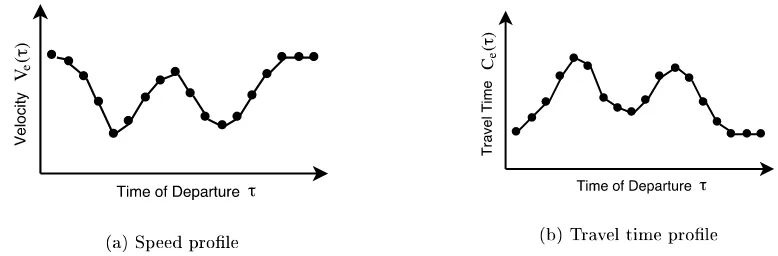
to compute historical speed proles, which is the average speed on an edge at a given time. Although in practice every edge has a unique speed prole, the third party aggregated the data to only 15,000 dierent speed proles. Each edge in the graph is linked to one of these speed proles, meaning multiple edges share the same speed prole. The speed proles predict the travel time at a certain moment in time on any of the graph's edges. Although it is just a prediction, we consider these proles as the real speeds in the road network.
Chapter 1. Introduction 6
[image:14.596.99.488.87.215.2](a) Speed prole (b) Travel time prole
Figure 1.2: (a) Possible speed prole over a day of a single edgeein graphG. ORTEC acquires the
speed proles from a third party. (b) The travel time proles results from the speed prole.
1.2.3 Current approach
So far we described two OR problems, the VRP and the SPP. The software program ORD is able to solve these two problems, giving customers the ability to plan their distribution processes eciently. ORD uses construction, destruction, and local search heuristics to automatically solve the VRP, and thereby creating a near optimal set of routes. In essence, these heuristics generate an enormous amount of possible plans, and at the end select the plan with the best set of routes. Transport planning at companies almost always includes time constraints, e.g., time windows at locations and drivers legislation. Therefore, to solve the VRP and make sure no constraints are violated, heuristics need (time-dependent) travel times of shortest paths between all pairs of consecutive locations within the routes.
The ORD software is divided into multiple components. We focus on the components Vehicle Routing Algorithm and Shortest Path Algorithm. We call these components COMTEC Vehicle Routing System (CVRS) and the Travel Time Calculator (TTC) respectively. The latter contains more functionality than solely calculating (TD)-TTs, but in this research we solely focus on the TD-TTs. We describe the CVRS and the TTC in Chapter 3.
The algorithm in the TTC returns an estimate of the TD-TT, using a tailor made method called the representative approach. This estimate favours a fast response, as speed is an important factor within solving the VRP. In theory, it is possible to get the exact TD-TT for each node pair in the graph using the representative approach, but this increase of the accuracy in the method quickly results in the need for an unusable amount of main memory. Currently, it is decided that the main memory usage of the TTC cannot exceed the 1000 MB. A detailed description of the representative approach is given in Section 3.2.
Getting the TD-TT between two locations is possible using an exact approach, but it takes a signicant amount of time to calculate it. The idea prevails that the current TD-SP algorithm does not return accurate travel times, and therefore creating infeasible and sub-optimal transport plans.
1.3 Problem Description
Chapter 1. Introduction 7
for solving the TD-SPP needs to be fast, and the algorithm only has to return the TD-TT and not necessarily the shortest path itself. For a more formal problem description of the TD-SPP, we refer the reader back to rst part of Section 1.2.1.
The representatives method proves to be a fast algorithm for TD-TT queries. The major drawback of this approach is that it is only an estimation of the TD-TT based on the static and deterministic TTFs. Estimating the TD-TT results in a dierence between what the vehicle routing algorithm (CVRS) uses and what is actually true based on the historical TTF. A signicant discrepancy in the travel time causes the route planning to be unrealistic and/or non-optimal. When the estimated travel times are too short, it causes drivers to be late and miss the agreed delivery times. When the estimated travel times are too long, we create unnecessary slack within the schedule.
We do not know what the eects are of using the representatives method. Therefore, we do not know ifi)the travel times are indeed suciently inaccurate, and ii) what the eects are on the functioning
of CVRS. This means, that it is possible that the travel times are actually quite accurate and it has no eect or only a small eect on the quality of the transport plans of CVRS. It is also possible that the estimation of the TD-TTs is poor, but that it has no eect on the quality of the transport plans.
1.4 Research Goal
The research goal of this study is to develop an improved algorithm that calculates the travel time between two points on a map, for any departure time. The algorithm has to be more accurate than the current implementation, without increasing the computation times too much and preferably with less memory use than the current method.
1.5 Research Scope
In this section, we specify some boundaries of our research. This research focusses on TD-TTs based on static and deterministic TTFs. Realized travel times are outside the scope of this research, we are not interested in improving the provided TTFs. This data is provided by a third-party company and we see it as the ground truth. It is their responsibility to provide as reliable data as possible. Also, dynamic travel times are outside the scope, meaning we solely focus on TTFs that are based on historical data. We are already able to extract the exact TD-TTs from the TTFs, using time-dependent Dijkstra's (see Section 2.1). This comes at the cost of large computation times, something that is not favourable for customers, but it is good enough for research.
Chapter 1. Introduction 8
1.6 Research Approach
To come to an appropriate answer for the problem and to reach the goal of this research, we formulate a number of research questions. We present our research questions, each with a small introduction to motivate its importance. Finally, we give an overview of our research approach.
First, we want to research what is currently known in literature about our research problem.
1. What is currently known in the literature about the use of TD-TTs in vehicle routing problems? (a) What kind of shortest path algorithms can be used to calculate TD-TTs from a weighted
graph where the non-negative edge weights are time-varying? (b) What kind of algorithms are closely related to the TTC?
Second, the TTC has never been evaluated thoroughly. Before developing a new algorithm, we want to assess the accuracy of the TTC. We want to know if it is even necessary to develop a new one. In addition, this helps us to get a better understanding in which situations the TTC performs better than in others.
2. How accurate are the calculated TD-TTs from the TTC?
(a) What is the dierence between the exact TD-TT and the TD-TT calculated by the TTC? (b) How does the number of representatives aect the accuracy of the TTC?
(c) How does the location of the origin and destination of a path aect the accuracy of the TTC? Third, we design an alternative algorithm that quickly calculates the TD-TTs to be used in the VRP. It is important that it ts the current ORD framework as well.
3. What algorithm is suitable to calculate the TD-TT of the shortest path quickly within a weighted graph where the non-negative edge weights are time-varying?
Fourth, we want to know the accuracy and the performance of the developed algorithm. We evaluate our algorithm by comparing it to the TTC, both on the relative travel time gap as computational speed. We use the same datasets and evaluation criteria as used in research question 2.
4. What is the accuracy and performance of the developed algorithm?
1.7 Research Outline
Chapter 2
Literature Review
This chapter describes the current state of literature related to our research. The following sections describe the path nding algorithms that are currently known within the literature. We compare these techniques using three variables, namely: speed-up, preprocessing time, and space overhead [6]. Speed-up is the factor to which the query time of a path nd algorithm is faster than Dijkstra's algorithm. The preprocessing time is the time needed to pre-process the representation of the graph used by the specic technique. Space overhead is the memory usage needed to store the representation of the graph. Often, techniques can be tuned among these variables, resulting in a trade-o between the three.
Section 2.1 describes the basic techniques for path nding within a graph. In Section 2.2, we look at the path nding techniques that use hierarchies to speed-up the query time. In Section 2.3, we discuss labelling algorithms that store information on nodes, for the retrieval of shortest paths or to successfully prune edges during the path search. Finally, in Section 2.4 we focus on path nding techniques that include time dependencies within the graph.
2.1 Basic shortest path algorithms
In this section, we discuss several path nding algorithms. The core of every algorithm is the in 1959 developed Dijkstra's algorithm, which guarantees to nd the shortest path in any graph. First we discuss Dijkstra's algorithm, and subsequently algorithms that add speed-up techniques, or add information to the graph to speed up the process as well.
Dijkstra: Already in 1956, Dijkstra developed an algorithm to determine the optimal path between two locations in a network [19]. The optimal path is the path with the least resistance between two vertices in a graph, which can be measured in, e.g., distance or time. Because the algorithm is relatively fast while giving optimal solutions, the algorithm is still used nowadays in many dierent type of routing problems.
The algorithm keeps a priority queue Q of all nodes in the graph, ordered by the total distance from
starting points. All node-to-node distances are initialized to innity, except the distance from nodesto
nodes, which is set to 0 and added to queueQ. During every iteration, the algorithm picks nodeufrom
the top of queue Q(node with least distance), and starts assessing all outgoing edges to all neighbour
Chapter 2. Literature Review 10
nodes. For each edge, it determines the distance from nodes, via nodeu, to the nodev at the other end
of the edge. If the distancestou, plus the length of the edge, is shorter than the current value of node v, it updates the value of node v. Afterwards, the updated node is added to the priority queueQ. All
visited nodes, until the target nodetis reached, are referred to as the search space of the Dijkstra query
of nodesto nodet. Dijkstra is applicable for all kind of graphs, as long as the edges have non-negative
values. Also, no pre-processing is necessary, making it easy to update the graph. However, in gigantic graphs the computational time of Dijkstra for nding the shortest path between start s and target t
becomes too high to be used conveniently.
Bi-directional Dijkstra: The search space used by Dijkstra can be reduced using bi-directional Dijkstra [20]. Instead of starting only at start-node s, the bi-directional search also does a backward Dijkstra
search from target-nodet. A backward search is similar to the normal Dijkstra search, but instead of
looking at all outgoing edges, the algorithm considers all incoming edges. In an undirected graph, the forward and backward search are identical, due to the characteristics of the graph. For road networks, bi-directional Dijkstra reduces the search space roughly to half the size of the unidirectional approach, making the algorithm twice as fast. Bi-directional Dijkstra has the same advantages and disadvantages as the regular Dijkstra. However, time-dependent path nding is not possible, as during the backward search it is known yet what the time of arrival is going to be.
A* Search: Hart et al. [21] propose a goal-directed version of Dijkstra's Algorithm. The idea of A* Search is to traverse the edges that are in the general direction of the target-node as early as possible. Instead of picking the nodeuout of priority queueQbased on solely the distance from start nodes to
that node u, it adds the estimated distance from nodeu to target nodet to that value. This way, the
nodes that are closer to the target, are picked rst. The estimating distance function can have dierent implementations. A possible implementation would be to calculate the euclidean distance based on the coordinates of the nodes. In practice, A* performs poorly compared to current modern techniques [22].
Geometric Containers: Schulz et al. [23] propose another goal-directed version of Dijkstra's Algorithm, called Geometric Containers (GC). The algorithm pre-computes an edge labelL(e)that contains information
on the target nodes that have edge(u,v) on their shortest path, given nodeu as the start node of that
shortest path. During a query, all edges that do not have target nodet in L(e), can be safely pruned.
Because it takes up too much memory space to save all nodes in every edge containers , the container contains geometric information on all nodes that have edge e on their shortest path. The geometric
information can be angular, like at Schulz et al. [23], but can also be shaped like ellipses or a convex hulls [24]. A large disadvantage is that for every nodeuin graphG, a one-to-many Dijkstra search has to be
completed during the pre-processing phase. This algorithm is commonly used within public transport networks, and not on road networks.
Arc Flags: The last goal-directed path nding algorithm we discuss, is Arc Flags (AF) [25,26]. During a pre-processing phase, the algorithm subdivides the graph intoKdierent cells. The areas are roughly
balanced in the number of nodes it contains, and have a small number of boundary edges. Each edge contains a vectorCiof lengthKbits, in which biticorresponds to celli. If the edge belongs to a shortest
path to cell i, ithbit in Ci is set to 1. During the search, the algorithm prunes the edges that do not
contain the cell in which target nodet belongs. The big advantage is that it is a relatively easy query
Chapter 2. Literature Review 11
2.2 Hierarchical shortest path algorithms
This section focusses on path nding techniques where the algorithm modies the graph in a preprocessing stage, to ensure faster queries. They are often called hierarchical techniques, as it transforms the original at graph into a multi layered graph to exploit the inherent hierarchy of road networks [22]. The time-dependent variant of the contraction hierarchies method is currently being researched at ORTEC to replace the highway node routing method.
Highway Hierarchies: Sanders and Schultes [28] were the rst to develop an algorithm that uses the hierarchical characteristics of the road network. Highway Hierarchies (HH) provides fast solutions, without losing the optimality Dijkstra has. This has to do with the typical characteristics of a road network, which bounds the need to have an algorithm that is applicable for all kinds of graphs. Highway Hierarchies starts with a preprocessing phase where the graph is modied to a graph with dierent hierarchical layers. These represent the same hierarchies we know in our road network, e.g., local access roads are lower in the hierarchy than highways. Note that the algorithm automatically nds the most important roads within the network, so the levels do not necessarily have to match the structure of the road designer. This pre-processing phase can take up several hours, but has to be calculated only once. The hierarchical graph allows for queries of trips of about 1 ms, which is considered very fast. The drawback of HH is that the travel time data is static, because no changes can be made to the graph without running the preprocessing phase again. Therefore, a typical HH-graph consists of only the free-ow travel times and all congestion is neglected. Also, even minor changes of the road network, result in completely reprocessing the HH-graph.
Highway Node Routing: Schultes and Sanders [29] developed a successor algorithm of HH, called (Dynamic) Highway-Node Routing (HNR). HNR solves the problem of having to recalculate the complete graph, even if only one edge changes. HNR allows for fast updates of minor changes in the hierarchical graph, with a speed of 2 40 ms (on the Western European map). Afterwards, this allows for fast queries of about 1 ms on average. A road network does not change that often, as it takes some time to construct new roads or upgrade them. Still, the graph contains only static travel times. Updating the graph after each query is not an option, as this results in updating all arcs within the graph. The query speed seems promising, but these speeds are only reached when just a few arcs are updated. Still, HNR is a predecessor of contraction hierarchies, that is in its core much simpler to implement.
Contraction Hierarchies: Geisberger et al. [16] developed the Contraction Hierarchies (CH) algorithm, which is a successor of HH and HNR. It is based on the idea of placing the more important nodes (the ones often on a shortest path) higher up the contraction graph than less important nodes. CH starts with a pre-processing phase, in which the nodes are one by one contracted from the original graph, in order of least important to most important. During the contraction of one nodeu from the graph, for
each incoming and outgoing node pair, CH checks if path< v, u, w >is the shortest path from nodev to
nodew. If so, this shortest path is added as a short-cut in the remaining graph. Afterwards, a query for
a (s, t)node pair is done with a forward upward Dijkstra search from node s, and a backward upward
Dijkstra search from nodet. One of the nodes where the two searches meet, is the node on which the
Chapter 2. Literature Review 12
2.3 Labelling shortest path algorithms
This section discusses the most recent developments in path nding techniques, called labelling methods. This technique precomputes labelL(v)for each nodev, which contains information on the shortest paths
within the graph. Using these labels results in successfully pruning edges that are not on a shortest path, or directly retrieving the distance of shortest path, without looking at the input graph.
Hub Labelling Algorithms: The Hub Labelling (HL) method pre-computes a label to every node
n∈V [30,31]. These labels contain information on the shortest path to a set of nodes, so that the labels
of both nodes L(s)andL(t), share at least one node. This way, a shortest path can be found for each
node pair(u, v), just by assessing the labels of both nodes. For directed graphs, two dierent label sets
for each node are computed; one for all outgoing edges, and one for all incoming edges.
Transit Node Routing: Bast et al. [32] based the development of the Transit Node Routing (TNR) algorithm on a few key observations. First, they observed for long distance travel, a particular start location has a few important trac junctions, for which all paths will use one of those access nodes. Second, each access node is relevant for several nodes in its proximity. The union of access points T of
all nodes in the graphV is small and is called the transit node set. The algorithm has a preprocessing
phase, where the algorithm identies the transit node set T ⊆V rst. Second, the complete distance
table between all access nodes in the transit node sets is calculated. Finally, for each node in graph V,
its access nodes are determined. A query is a simple search of the smallest distance to each access node of both the start and target node and the distance between two access nodes. TNR seems to be a good starting point for our time-dependent path nding algorithm. However, as far as we know, it has never been tested on graphs with time-dependent edge weights.
Pruned Highway Labelling: Akiba et al. [33] developed the Pruned Highway Labelling (PHL) algorithm, which can be seen as a hybrid between a labelling algorithm and transit node routing. First, the algorithm preprocesses the graph into several dierent shortest paths. For each nodesin graphV a label is created,
so any shortest s−t path can be expressed as < s−u−w−t >, where < u−w >is a subpath of a
pathP that belongs to the labelssandt[22]. PHL is one of the fastest algorithms for querying shortest
path. However, it has only been evaluated on undirected graphs.
2.4 Time dependent shortest path algorithms
Within this section we focus on time dependent path nding techniques. These techniques consider the variation in travel cost during a day.
Chapter 2. Literature Review 13
Time-Dependent Contraction Hierarchies: Contraction hierarchies already proved to be extremely ecient for graphs with static travel times. Time-dependent Contraction Hierarchies (TD-CH) is a variant that includes time-dependent edge weights in the road network. It is the rst hierarchical path nding technique for time-dependent paths that allow for bidirectional queries. Time-dependent contraction hierarchies is extremely useful even with larger graphs, and outperforms other TD-PF algorithms in the case of considerable time-dependence on the edges (map: Germany, weekdays). Unfortunately, the current implementation requires still too much memory during the preprocessing phase to be realistic to be implemented yet.
Customizable Route Planning: Delling and Wagner [27] developed Customizable Route Planning (CRP) with the idea to make an ecient real-world routing engine. It should incorporate turn restrictions, avoidance of U-turns, avoid left turns, avoid/prefer highways, and using dierent modes of transportation like biking and walking. This using as little memory as possible. Still, the algorithm should allow for fast graph updates and one-to-one queries. CRP has two preprocessing phases. First, a metric-independent phase only considers the topology of the graph, which is the data that changes very infrequently like edge distance, number of lanes, etc.. The second phase, metric customization, transforms the metric-independent data into a single metric. This single metric can change quite often, therefore the second phase takes a few seconds to complete. The preprocessing phase results in multilevel nested partitions. Within these partitions, or cells, shortcuts are inserted between the boundary nodes, so queries can skip the nodes within the cells in which the start or target node are not presented. The algorithm is able to get fast queries, but not as fast as the fastest existing methods currently known. However, the queries of CRP are robust and suitable for all above dened real-world requirements. Time dependent queries are possible due to real-time trac updates of the graph. This feature is useful for real-time planning, but the updating phase takes to long to be useful during optimization, making it irrelevant for our purpose.
2.5 Conclusion
We gave an overview of the possible techniques available to solve a travel time query. The basic path nding techniques are not fast enough to handle large amounts of time-dependent travel time queries. However, these simple techniques are often used as a part of more sophisticated algorithms, like the ones we presented in Sections 2.2, 2.3, and 2.4. Table 2.1 presents the memory space usage per node, preprocessing time, and speed-up compared to Dijkstra of the discussed algorithms. The memory space and speed-up indicators are adjusted to be experiment setup independent, by using relative values. Memory space is measured in byte per node, in which the node is a node on the map. The speed-up is measured by comparing the algorithm's running time with the running time of Dijkstra's algorithm using the same setup, making the speed of the computer irrelevant. Keep in mind that the preprocessing time is the absolute value, so dierences occur due to the use of a dierent setup. We were not able to nd all values for the discussed algorithms, these values are therefore absent in Table 2.1.
Chapter 2. Literature Review 14
method memory space preprocessing speedup source [b/node] [min] [comp. to Dijkstra]
Dijk. 24 0 1 (1)
BDD 24 0 2 (1)
A* - - -
-GC - - -
-AF 36 20 6.2∗103 (1)
HH 72 13 10∗103 (2)
HNR 26 15 7.1∗103 (2)
CH - 5 23∗103 (1)
HL 1121 37 4.6∗106 (1)
TNR 149 20 2.0∗106 (1)
PHL 828 50 2.5∗106 (3)
TDD 24 24 1 (1)
TD-CH 523 285 1.8∗103 (2)
[image:22.596.137.462.81.299.2]CRP 54 60 1.5∗103 (1)
Table 2.1: Overview of the path nding algorithms. For all algorithms, the Western European map from PTV AG was used. For A* and geometric containers no data was available. Source (1): Bast
et al. [22]. Source (2): Batz [6]. Source (3): Akiba et al. [33].
Chapter 3
Current Methods
In this chapter we discuss the current Vehicle Routing Problem (VRP) and Time Dependent Shortest Path Problem (TD-SPP) solving methods of ORTEC. In Section 3.1 we give a brief overview of the working of the COMTEC Vehicle Routing System (CVRS). In Section 3.2 we describe in more detail the function of the shortest path algorithm and travel time calculation within the Travel Time Calculator (TTC).
3.1 Vehicle Routing Algorithm (CVRS)
This part is condential.
3.2 Time Dependent Shortest Path Algorithm (TTC)
This part is condential.
Chapter 4
Benchmarking
This chapter describes the experiments we use to (i) research the eects of time dependent travel times on vehicle routes and to (ii) provide a benchmark of the TTC, to later compare with our algorithm. In Section 4.1 we describe the data we use in our experiments. Section 4.2 describes the evaluation criteria used in the experiments. In Section 4.3, we describe the dierent experiments we conduct. Section 4.4 describes the results of the experiments. Finally in Section 4.6, we draw our conclusions based on the results.
4.1 Data
This section discusses the three dierent types of data we need to carry out our experiments. The rst subsection describes the map data, containing the graph and travel time proles of the road network. In the second subsection we describe the test sets containing the origin and destination pairs to test the TTC and our algorithm. The last subsection describes the representatives that the TTC uses to approximate the time dependent travel times.
4.1.1 Map
The map consist of the complete road network of the BeNeLux, including the main roads of the regions of Northern France and West Germany. Figure 4.1a shows this map, including the congestion information of a Tuesday. The complete graph consist of 3,114,941 nodes and 6,636,596 edges. Each edge is connected to seven speed proles, which correspond to the seven days in a week. In total 15,754 dierent speed proles exist, meaning many edges share the same speed prole. To calculate the time dependent travel time, the speed at the time of departure over the edge is retrieved from the speed prole of that edge, and divided by the length of that edge. Within the road network, 3,727,986 edges have at least one day with a variating speed prole. This means 2,908,610 edges have no congestion, or no congestion was measured. 2,242,591 edges have congestion every day of the week. Figure 4.1b shows the percentages of the edges that have no, partly, or full congestion information. It shows that the majority of the road types have congestion data available. Figure 4.3 in Section 4.1.2 shows the zoomed road networks of four congested areas, where clearly congestion is visibly on the main road around the city. This means
Chapter 4. Benchmarking 17
that the provided map consist mainly of edges with non-constant speed proles, making time dependent queries useful.
(a) Road network
0% 20% 40% 60% 80% 100%
Motorway A-road A-road (city) B-road B-road (city) Regional road Regional road (city)Local road Local road (city)Other road Other road (city)Pedestrians Ferry
Occurence
No congestion Partly congestion Every day congestion
[image:25.596.78.502.124.313.2](b) Distribution of speed proles
Figure 4.1: (a) Overview of the congestion of the BeNeLux map on a Tuesday. The colors go from light green which mean no congestion via yellow, orange, red, purple, and black to the heavy congested areas. It shows that the BeNeLux part has a dense road network, while the parts in France and Germany only consist of the main roads. (b) The percentages of the edges that have no congestion, partly congestion, or have non-constant speed proles for all 7 days. The percentages are categorized
into the dierent road types of the graph.
4.1.2 Test sets
To eectively get a benchmark of the current algorithm (TTC) and to test the functioning of our algorithm, we dene three dierent test groups. In total, the three test groups have 15 test sets of 2500 randomly selected Origin-Destinations pairs. We assume that a set of 2500 shortest paths is sucient to draw conclusions based on the average values we calculate. We base all our test sets on a graph with edges containing truck speeds, as the majority of the customers of ORD use trucks as well. This means that all travel times are truck travel times.
Test group 1: Path lengths
We randomly generate seven test sets in test group 1, each consisting of 2500 dierent Origin-Destination (O-D) pairs. All O-D pairs in a single set have the same shortest free ow path length. As we explain later in this thesis, we use these test sets to study the relationship between the distance of a path and the accuracy of the TTC.
Chapter 4. Benchmarking 18
of the node pair. Hence, the test set that consists of shortest paths with a length of 10 minutes, is called 10-minute path length.
Test group 2: Vicinity of representatives
In test group 2, we randomly generate four test sets, each consisting of 2500 dierent Origin-Destination (O-D) pairs. All nodes in the test set, both origin and destination, have the same length from their representative. We use these test sets to study the relationship between the vicinity of the representatives and the accuracy of the TTC.
We use 220 representatives that are evenly distributed over the graph in a grid structure. We refer the reader to the next section for more information on the representatives. The test sets are created as follows. First, we randomly select two representatives out of the set of 220. Second, we run the Dijkstra algorithm twice, both have either one of the representatives as initial node. The Dijkstra algorithm continues until the distance between the source node and a target node exceeds the predetermined length of the test set. The two resulting target nodes of both runs, will be either the origin or destination node of the O-D pair. Afterwards, this process is repeated. In this way, all nodes of all O-D pairs within one test set have the same length towards the nearest representative. We name the test sets after the vicinity of the O-D to the representative. Hence, the test set that consist of O-D pairs that are at ve minute distance from their representatives, is called 5-minute vicinity length .
The result of the Dijkstra algorithm with a representative as initial node, will always result in the same selected node after the test set length. The limited amount of representatives compared to the number of O-D pairs in the test set causes the O-D pairs to be limited to 220 dierent nodes. To overcome this problem of always selecting the same node from the Dijkstra queue for each representative, we randomize the lengths by a half percent. In that way, the Dijkstra algorithm quits after slightly dierent lengths, resulting in selecting a dierent node from the queue. The randomization is low enough, to not cause major variation in the test sets due to dierent lengths from the representatives. The vicinity lengths of test sets are 5 min, 10 min, 15 min, 20 min.
Test group 3: Congested areas
Chapter 4. Benchmarking 19
Figure 4.2: Displays the shortest paths of the 5% O-D couples within test set Path length 10 min. with the highest level of delay. We observe major concentrations of paths around the major cities in
The Netherlands, Belgium, Luxembourg, and the Rhine-Ruhr region.
We observe major concentrations of paths around the major cities in The Netherlands, Belgium, Luxembourg, and the Rhine-Ruhr region. Luxembourg only show a few paths, and the Rhine-Ruhr region is the part of the map with a more sparse network. We make a selection of the cities in Belgium and The Netherlands, and we pick Amsterdam, Antwerp, Brussels, and Rotterdam to be the areas we select the test sets from. We use these test sets to study the eect on the accuracy of the TTC of having trips in a congested area. We name the test sets after the area they represent. Figure 4.3 shows the congestion on the road networks of the four areas.
(a) Amsterdam (b) Antwerp
(c) Brussels (d) Rotterdam
Figure 4.3: Overview of the congestion of the dierent urbanized areas. The colors go from light green which mean no congestion via yellow, orange, red, purple, and black to the heavy congested areas. Note
[image:27.596.98.531.406.737.2]Chapter 4. Benchmarking 20
We select the O-D-pairs in the test sets by randomly selecting two nodes within the chosen areas. This results in O-D pairs that dier in the length of their shortest path, and the vicinity to their representative. All O-D pairs within one test set have in common that their origin and destination nodes are within a certain area.
Overview:
Table 4.1 shows an overview of all 15 test sets. Every test set consist of 2500 O-D pairs and are selected within the area of (49.316,2.581) and (53.473,7.483). Test group 3 consist of O-D pairs selected in even smaller areas, these areas are presented in column four of Table 4.1.
Testgroup 1: Testgroup 2: Testgroup 3: Path length Vicinity length Congested area
10 min. 5 min. Amsterdam (52.18,4.74)(52.58,5.24) 20 min. 10 min. Antwerp (51.05,4.13)(51.45,4.63) 30 min. 15 min. Brussels (50.60,4.10)(51.00,4.60) 60 min. 20 min. Rotterdam (51.75,4.15)(52.15,4.65) 120 min.
180 min. 240 min.
Table 4.1: Overview of the 3 test groups and 15 test sets. All test set consist of 2500 O-D pairs. Test group 1 and 2 consist of nodes selected within the area of (49.316,2.581) and (53.473,7.483). Test group
3 has dierent areas, the fourth column presents the coordinates of these areas.
4.1.3 Representatives
We use both representative (grid and address) strategies for our benchmarking experiments. The grid strategy is normally used for demo purposes only, while the address strategy is implemented at clients. However, we nd it useful to use the grid strategy for our experiments as it provides an independent set of representatives that is not related to a particular set of addresses. Besides, it is unknown how the grid strategy performs, so it provides useful insights. The grid strategy selects representatives within the area of (49.316,2.581) and (53.473,7.483). These make roughly the outside border of the BeNeLux. This means that the edges outside of the BeNeLux are mainly mapped to the representatives at the border. The selected representatives are evenly distributed over the map, creating a grid-like structure.
Chapter 4. Benchmarking 21
4.2 Evaluation criteria
In this section, we dene the criteria we use to evaluate the accuracy of the travel time algorithm. First, we dene the notations that helps us explain the criteria. Please note, that we continue using the notations of Section 1.2.1.
Consider a node pairu, as a pair consisting of an origin nodeoand destination noded, where both nodes o, d∈V. LetU be the set of one or multiple node pairs u. Pathpod is a path betweeno andd, where
path< o→...→d >consists of nodes that are within graphG= (V, E). Wheno, d=u, thenpod=pu.
Podis the set of all pathpod betweenoanddandPU is the set of all paths of allodpairs in set U.
Pathqod is the shortest path between oandd, where all edgese∈E of graphGhave a constant travel
timete. We dene this constant travel time as the free ow travel time t0e of edge e. We deneQod as
the set of shortest pathsqod, which in this case meansqod=Qodas there is only one shortest path. QU
is the set of all shortest paths of allodpairs in setU.
Path rodτ is the shortest path betweeno anddat departure time τ, where all edgese∈E of graphG
have a Travel Time Function (TTF) te(τ). te(τ)is the cost of traveling edgeewhen starting at timeτ.
Rodτ is the set of all paths Rodτ betweeno anddat departure timeτ. RU τ is the set of all paths of all
odpairs in setU at departure time τ.
Next, we dene three dierent variants of the travel time between two nodeso and d. First, we dene T0(pod)as the free ow travel time over path pod. Second, we dene T(qod, τ) as the time dependent
travel time over shortest pathqodat departure timeτ. Note thatqod is the shortest path over edges with
t0
e, while the travel time is calculated with thete(τ)of the shortest path edges. Last, we deneT(rodτ, τ)
as the time dependent travel time over shortest pathrodat departure time τ.
We decide to use three evaluation criteria to evaluate the performance of the TTC. The criteria are the level of delay, the travel time gap, and shortest path share with shortest path of representatives. We discuss them in the following paragraphs. To clarify the criteria, we use an example graph, we present in Figure 4.4. This graph consist of six nodes and eight edges. Nodeorepresents the origin and noded
represents the destination. Noderoandrd represent the two representatives in the graph. Each edge in
the graph has a constant travel time and a time dependent travel time, represented by {t0
e,i→te(τ)}.
We retrieve thete(τ)from the matrixtτ,i, by looking at theivalue of the edge and departure timeτ at
which the edge is traversed.
Level of delay:
The level of delay is the dierence in percentage between the time dependent travel time and the free ow travel time. It is an indicator of congestion, as a higher delay indicates more congestion. Consider
T(qodτ)as the time dependent travel time andT0(qod)as the free ow travel time. We dene the level
of delay between the nodeso anddat departure time τ asLoDod(τ). Therefore, the equation is:
LoDod(τ) =
T(qod, τ)−T0(qod,0)
T0(q
Chapter 4. Benchmarking 22 B ro A o C D d E F rd {4,2} {6,2} {2,0} {3,1} {2,0} {4,1} {1,0} {5,2} (a) Graph
tτ,i=
2 3 4
2 3 4
3 7 5
3 7 5
2 6 5
2 6 5
1 5 4
1 5 4
(b) Travel time functions
Figure 4.4: (a) A graph consisting of 6 nodes and 8 edges. Each edge consist of {t0e,i→te(τ)}. The
rst value is the free ow travel time, the second value refers to column in the matrix of (b). Thus, multiple edges share the same travel time function.
To calculate the average level of delay over a set of node pairsU, we use the following equation:
LoDU(τ) =
X
od∈U
T(qod, τ)−T0(qod)
X
od∈U
T0(q
od)
(4.2)
To clarify, we provide an example using Figure 4.4. We calculate the level of delay between node A (origin o) and node D (destinationd) at departure time 0. The shortest pathqod is< A→B →D >,
which has aT0(q
od)of4 + 3 = 7. TheT(qod,0)uses the same shortest path, but uses the time dependent
travel times of the edges. Therefore,T(qod,0) = 4 + 6 = 10. The level of delay is therefore 107−7 = 0.429.
Travel time gap:
The travel time gap is the dierence between the time dependent travel time and the travel time calculated by the TTC [14]. A smaller gap means a smaller dierence between the calculated travel time and the actual travel time and thus yields higher accuracy. There are two dierent ways to calculate the travel time, using two dierent ways to compute the shortest path betweeno and d. Therefore, we have two
dierent travel time gap criteria as well. We dene the travel time gap betweeno and d over the free
ow shortest path at departure timeτ as:
T T Gf fod(τ) =|T T C(od, τ)−T(qod, τ)
T(qod, τ)
| (4.3)
Therefore, we have two dierent travel time gap criteria as well. We dene the travel time gap between
oanddover the time dependent shortest path at departure timeτ as:
T T Gtdod(τ) =|T T C(od, τ)−T(rod, τ)
T(rod, τ)
Chapter 4. Benchmarking 23
To calculate the average travel time gaps over a set of node pairsU, we use the following equations:
T T Gf fU (τ) = X
od∈U
|T T C(od, τ)−T(qod, τ)|
X
od∈U
T(qod, τ)
(4.5)
T T Gtd U(τ) =
X
od∈U
|T T C(od, τ)−T(rod, τ)|
X
od∈U
T(rod, τ)
(4.6)
To clarify, we provide an example using Figure 4.4. We calculate theT T Gf f between node A and node
D at departure time 0. The shortest pathqod is< A→B →D >, which has aT0(qod,0)of4 + 3 = 7.
TheT T C(A, B,0) returns a value of 8. Therefore,T T Gf fod(0)is|8−7
7 |= 0.142.
We calculate theT T Gtd using the same node pair and departure time. The shortest pathrod is< A→
B →C →D >, which has a T(qod,0) of 4 + 6 = 10. Because the TTC is a black box, let us in this
example assume theT T C(A, B,0)returns a value of 8. Therefore,T T Gtd od(0)is|
8−10 10 |= 0.2.
Calculating theT T Gtd
od(τ)is a computational dicult task and this takes a tremendous amount of time.
This makes extensive testing impossible, as it simply takes too much time. We argue that it is accurate enough to base our nal results and conclusions solely on theT T Gf fod(τ)instead of the T T Gtd
od(τ). We
conduct a preliminary experiment to research the loss in accuracy using the T T Gf fod(τ) instead of the T T Gtdod(τ). For this experiment, we use test group 1 that is reduced from 2500 O-D pairs to 250 O-D
pairs, as using 2500 would takes too much time to compute. We use two representing weekdays (Tuesday and Thursday) and two representing moments during morning and afternoon rush hour (8:00 and 17:00). The preliminary experiment shows that the implications are relatively small, and stay well beneath 2.5%. Figure 4.5 shows the average absolute dierence between the time dependent travel time over the free ow shortest path and the time dependent travel time over the time dependent shortest path.
8:00 17:00 0% 1% 2% 3% 4% 5%
Departure time (hh:mm)
| T T G f f od ( τ ) − T T G td od ( τ ) | 10 min. 20 min. 30 min. 60 min. 120 min. 180 min. 240 min.
Figure 4.5: Percentage dierence of the absolute dierence between theT T Gf fod(τ)andT T Gtdod(τ)of
250 O-D pairs per test set. The O-D's in the test sets dier in free ow path length between the origin and destination.
Shortest path share with shortest path of representatives:
This evaluation criterium indicates the percentage of shared shortest path between node o and d, and
Chapter 4. Benchmarking 24
paths, and dividing it by the total length of all unique edges present in both shortest paths. We dene the Path Sharings Percentage (PSP) as:
P SPod=
X
e∈qod∩e∈qrord
t0
e
T0(q
od,0) +T0(qrord,0)−
X
e∈qod∩e∈qrord
t0
e
∗100% (4.7)
To clarify, we provide an example using Figure 4.4. The shortest free ow path between o and d is < A→B →D >. The shortest free ow path between ro andrd is < B→D →F >. The total free
ow travel time between A and B equals4 + 3 = 7, while the total free ow travel time betweenro and
rd is3 + 1 = 4. Edge BD is present in both shortest free ow paths, with a length of3. Therefore, the
shared percentage is 3
7+4−3 = 0.429.
4.3 Setup of the experiments
In the following subsections, we describe the experiments in more detail.
4.3.1 Experiment 1: The eect of the path length on the time dependent
travel time over dierent departure times during the day
Introduction: In the rst experiment, we study the eect of dierent path lengths on the variability of the time-dependent travel time. We expect that an increase in path length leads to less variation of the travel time over the departure times, as well as a decrease in the travel time gap. We use the Path lengths test set for this experiment.
Chapter 4. Benchmarking 25
Experiment 1.1
Test sets Path lengths: 10 min, 20 min, 30 min, 60 min, 120 min, 180 min, 240 min
Representatives 20 by 20, grid strategy f Map BeNeLux
Criteria Level of Delay, Travel Time Gap
Table 4.2: Overview of experiment 1.1
4.3.2 Experiment 2: The eect of the vicinity of the representative on the
time dependent travel time over dierent departure times during the
day
Introduction: In the second experiment, we study the eect of the vicinity of a representative on the travel time gap. We expect that paths that have their start and target nodes closer to their corresponding representatives have a lower travel time gap.
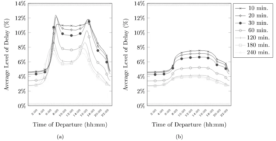
Calculation: We calculate for each O-D pair and each 15-minute interval, the time dependent travel time over the free ow shortest path. We compare the time dependent travel time with the free ow travel time to see the absolute dierence. The time dependent travel times should follow a congestion pattern with a clear morning and afternoon peak. The time dependent travel times of all four vicinity test sets should be equal, as they are randomly selected. Afterwards, we retrieve the travel times calculated via the TTC. The dierences between those travel times and the time dependent travel times is the so-called travel time gap. We take the average over two workdays (Tuesday and Thursday) and two weekend days (Saturday and Sunday) to see the eects of congestion over the week as well.
Experiment 2.1
Test sets Vicinity length: 5 min, 10 min, 15 min, 20min Representatives 20 by 20, grid strategy
Map BeNeLux
Criteria Travel Time Gap
Table 4.3: Overview of experiment 2.1
4.3.3 Experiment 3: The eect of congestion on the time dependent travel
time over dierent departure times during the day
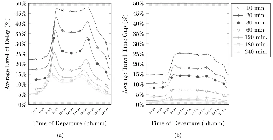
Chapter 4. Benchmarking 26
Calculation: We calculate for each O-D pair and each 15-minute interval, the time dependent travel time over the free ow shortest path. We compare the time dependent travel time with the free ow travel time to see the level of delay. We expect the level of delay over a day to have a clear morning and afternoon rush hour peak, which is a typical congestion pattern. Afterwards, we retrieve the travel times calculated via the TTC to calculate the travel time gap. We expect the travel time gap to be higher at the congested places and moments. We take the average over two workdays (Tuesday and Thursday) and two weekend days (Saturday and Sunday) to see the eects of congestion over the week as well.
Experiment 3.1
Test sets Amsterdam, Antwerp, Brussels, and Rotterdam. Representatives 20 by 20, grid strategy
Map BeNeLux (The areas of the test sets are a sub portion of the map)
Criteria Level of Delay, Travel Time Gap
Table 4.4: Overview of experiment 3.1
4.3.4 Experiment 4: The eect of the number of representatives on the time
dependent travel time over dierent departure times during the day
Introduction: In the fourth experiment, we study the eect of the number of the used representatives. We expect that a higher number of representatives results in a lower travel time gap.
Calculation: To study the eect of the number of representatives on the travel time gap, we take the test sets with the highest levels of delay because these are better for comparison. Therefore, we use the Brussels area and 10-minute path length test set. We vary the number of representatives to research the eects. The four sets of representatives are all selected using the grid strategy and consist of 57 (10x10), 220 (20x20), 519 (30x30), and 889 (40x40) representatives. We refer the reader back to Section 4.1.3 for a more detailed explanation of the sets of representatives. We calculate for each O-D pair and each 15-minute interval, the travel time gap. We only accumulate two workdays (Tuesday and Thursday), because we are not interested in the eects of the dierent levels of congestion over the week.
Experiment 4.1
Test sets Brussels area, Path lengths: 10 min
Representatives 10 by 10, 20 by 20, 30 by 30, and 40 by 40 grid strategy
Map BeNeLux (The areas of the test sets are a sub portion of the map)
Criteria Travel time gap