Computation of the drift velocity of spiral waves using response functions

University of Warwick institutional repository: http://go.warwick.ac.uk/wrap

This paper is made available online in accordance with

publisher policies. Please scroll down to view the document

itself. Please refer to the repository record for this item and our

policy information available from the repository home page for

further information.

To see the final version of this paper please visit the publisher’s website.

Access to the published version may require a subscription.

Author(s): I. V. Biktasheva, D. Barkley, V. N. Biktashev and A. J.

Foulkes

Article Title: Computation of the drift velocity of spiral waves using

response functions

Year of publication: 2010

Link to published article:

http://dx.doi.org/10.1103/PhysRevE.81.066202

Computation of the drift velocity of spiral waves using response functions

I. V. Biktasheva

Department of Computer Science, University of Liverpool, Ashton Building, Ashton Street, Liverpool L69 3BX, United Kingdom

D. Barkley

Mathematics Institute, University of Warwick, Coventry CV4 7AL, United Kingdom

V. N. Biktashev

Department of Mathematical Sciences, University of Liverpool, Mathematical Sciences Building, Peach Street, Liverpool L69 7ZL, United Kingdom

A. J. Foulkes

Department of Computer Science, University of Liverpool, Ashton Building, Ashton Street, Liverpool L69 3BX, United Kingdom

共Received 21 January 2010; published 1 June 2010兲

Rotating spiral waves are a form of self-organization observed in spatially extended systems of physical, chemical, and biological nature. In the presence of a small perturbation, the spiral wave’s center of rotation and fiducial phase may change over time, i.e., the spiral wave drifts. In linear approximation, the velocity of the drift is proportional to the convolution of the perturbation with the spiral’sresponse functions, which are the eigenfunctions of the adjoint linearized operator corresponding to the critical eigenvalues␭= 0 ,⫾i␻. Here, we demonstrate that the response functions give quantitatively accurate prediction of the drift velocities due to a variety of perturbations: a time dependent, periodic perturbation 共inducing resonant drift兲; a rotational symmetry-breaking perturbation共inducing electrophoretic drift兲; and a translational symmetry-breaking per-turbation共inhomogeneity induced drift兲 including drift due to agradient,stepwise, andlocalized inhomoge-neity. We predict the drift velocities using the response functions in FitzHugh-Nagumo and Barkley models, and compare them with the velocities obtained in direct numerical simulations. In all cases good quantitative agreement is demonstrated.

DOI:10.1103/PhysRevE.81.066202 PACS number共s兲: 82.40.Bj, 82.40.Ck, 87.10.⫺e, 02.70.⫺c

I. INTRODUCTION

Spiral waves are types of self-organization observed in physical 关1–3兴, chemical 关4,5兴, and biological 关6–11兴 sys-tems, where wave propagation is supported by a source of energy stored in the medium. The interest in the dynamics of spiral waves has significantly broadened in the last decade as the development of experimental techniques has permitted them to be observed and studied in an ever increasing num-ber of diverse systems such as magnetic films 关12兴, liquid crystals 关13兴, nonlinear optics 关14,15兴, novel chemical sys-tems关16兴, and in subcellular关17兴, tissue关18兴, and population biology关19兴.

In the ideal unperturbed medium, the core of a spiral wave may be anywhere, depending on initial conditions. However, real systems are always subject to a perturbation. A typical result of a symmetry-breaking perturbation is drift of the spiral waves, which has two components, temporal drift, which is shift of spiral wave rotation frequency, and spatial drift, that is slow movement of the spiral’s rotation center. The drift of spiral waves, particularly the spatial drift, is of great practical interest to applications. In cardiac tissue, drift of re-entry circuits may be caused by internal tissue inhomogeneities, or by external perturbations, such as elec-trical stimulation. The possibility of control of arrhythmias by weak electrical stimulation has been a subject of intensive research for decades.

Understandably, the drift of spiral waves was mostly stud-ied in the Belousov-Zhabotinsky reaction, which is the

easi-est excitable system for experimental study, and in the heart tissues and tissue cultures, which represents the most impor-tant application area. Examples of drift observed in experi-ments and numerical simulations include “resonant” drift caused by 共approximately兲 periodic modulation of medium properties through external forcing 关20兴, constant uniform electric field that causes electrophoresis of charged ions tak-ing part in the chemical reactions 关21兴, a spatial gradient of medium properties 关22–25兴 and pinning 共anchoring, trap-ping兲to a localized inhomogeneity关26–28兴. Interaction with a localized inhomogeneity can be considered to be a particu-lar case of the general phenomenon of vortex pinning to material defects, ranging from convective microvortex fila-ments in nanosecond laser-matter interaction to magnetic flux strings in the Sun’s penumbra 关29兴. A most intriguing property of spiral waves is that despite being propagating waves affecting all accessible space, they, or rather their cores, behave as pointlike objects.

Correspondingly, three-dimensional extensions of spiral waves, known as scroll waves, act as stringlike objects. There have been severalad hoctheories of drift of spiral and scroll waves exploiting incidental features in selected mod-els, e.g., 关30–33兴. Our present study is based on an asymptotic theory applicable to any reaction-diffusion sys-tem of equations in which a rigidly rotating spiral wave so-lutions exist. The theory was first proposed for autonomous dynamics of scroll waves for the case of small curvatures and small twists 关34,35兴 and then extended to the drift of spiral waves in response to small perturbations关36兴. In this theory,

the particlelike behavior of spirals and stringlike behavior of scrolls corresponds to an effective localization of so called response functions 共RFs, see exact definition later in this paper兲. The localization of RFs is the crucial assumption, which underpins the entire analysis. Originally 关37兴 this property was only a conjecture based on the phenomenology of spiral waves in experiments and numerical simulations 关31,38–40兴. The analytical calculation of the response func-tions appears to be infeasible. Numerical calculafunc-tions in the Barkley model关41兴and the complex Ginzburg-Landau equa-tion共CGLE兲 关42兴have confirmed that indeed they are essen-tially localized in the vicinity of the core of the spiral. The asymptotic theory based on the response functions has been successfully used to quantitatively predict drift of spirals, for resonant drift and drift due to parametric inhomogeneity in the CGLE 关43–45兴 and for drift in response to a uniform electric field in Barkley model关46兴. Despite this success, so far the asymptotic theory has not become a generally used tool for the prediction of spiral wave drift. This is partly due to difficulties in the numerical calculation of the response functions. In our recent publication 关47兴we have presented an efficient numerical method of calculating response func-tions in an arbitrary model with differentiable right-hand sides. The complexity of calculating response functions with this method is similar to the complexity of calculating spiral wave solutions themselves. In the present paper, we describe the application of the asymptotic theory using the response functions for the prediction of several types of drift and show how it works for two of the most popular generic excitable models, the FitzHugh-Nagumo 共FHN兲 system关48–50兴, and the Barkley system关51兴. We demonstrate that predictions of the asymptotic theory are in good quantitative agreement with direct numerical simulations. In addition, we demon-strate that the response functions are capable of predicting nontrivial qualitative phenomena, such as attachment of spi-ral waves to stepwise inhomogeneity and orbital movement around a localized inhomogeneity.

The structure of the paper is as follows. In Sec. II, we briefly recapitulate the asymptotic theory of the drift of spiral waves in response to small perturbation and present explicit expressions for drift parameters in terms of the spiral wave’s response functions for several sorts of drift. In Sec. III, we describe the numerical methods used for calculating the re-sponse functions, for direct numerical simulations, and for processing of the results. The results are described in Sec.IV. We conclude the paper by discussion of the results and their implications in Sec.V.

II. THEORY

A. General

We consider reaction-diffusion partial differential equa-tions,

⳵tu=f共u兲+Dⵜ2u, u,f苸Rᐉ, D苸Rᐉ⫻ᐉ, ᐉⱖ2,

共1兲 whereu共rជ,t兲=共u1, . . . ,uᐉ兲Tis a column-vector of the reagent concentrations, f共u兲=共f1, . . . ,fᐉ兲T is a column-vector of the

reaction rates,D is the matrix of diffusion coefficients, and r

ជ苸R2 is the vector of coordinates on the plane.

A rigidly clockwise rotating spiral wave solution to Eq. 共1兲has the form

U=U_„␳共rជ−Rជ兲,␽共rជ−Rជ兲+␻t−⌽_…, 共2兲

where Rជ=共X,Y兲T _{is the center of rotation, ⌽ is the initial} rotation phase, and ␳共rជ−Rជ兲,␽共rជ−Rជ兲 are polar coordinates centered at Rជ. For a steady, rigidly rotating spiral,Rជ and⌽ are constants. The system of reference co-rotating with the spiral’s initial phase and angular velocity ␻around the spi-ral’s center of rotation is called the system of reference of the spiral. In this system of reference, the polar angle is given by

␪=␽+␻t−⌽, with Rជ= 0 and⌽= 0. In this frame, the spiral wave solutionU共␳,␪兲does not depend on time and satisfies the equation

f共U兲−␻⳵␪U+Dⵜ2U=0, 共3兲

where the unknowns are the field U共␳,␪兲 and the scalar␻. In a slightly perturbed problem

⳵tu=f共u兲+Dⵜ2u+⑀h, h苸Rᐉ, 兩⑀兩Ⰶ1, 共4兲 where ⑀h共u,rជ,t兲 is some small perturbation, spiral waves may drift, i.e., change rotational phase and/or center location. Then, the center of rotation and the initial phase are no longer constants but become functions of time, Rជ=Rជ共t兲 and ⌽=⌽共t兲. In the co-rotating system of reference, time depen-dence will take form of a phase depending on time ␾共t兲 =␻t−⌽共t兲.

Thus, we consider three systems of reference: 共1兲laboratory,共rជ,t兲;

共2兲co-moving,共␳,␽,t兲, where共␳,␽兲=(␳共rជ−Rជ兲,␽共rជ−Rជ兲)

is the polar coordinate system centered at Rជ;

共3兲 co-rotating, 共␳,␪,␾兲, where ␪=␽共rជ−Rជ兲+␾共t兲 is the polar angle, and ␾=␻t−⌽共t兲 is the rotational phase, replac-ing time.

We shall look for a solution to Eq. 共4兲 in the form of a slightly perturbed steady spiral wave solution

U˜共␳,␪,␾兲=U共␳,␪兲+⑀g共␳,␪,␾兲,

whereg苸Rᐉ, 0⬍⑀Ⰶ1. Then, assuming that

Rជ˙,⌽˙ =O共⑀兲,

at leading order in⑀, the solution perturbation gwill satisfy the linearized system

共␻⳵␾−L兲g=H共U,␳,␪,␾兲, 共5兲

where

H共U,␳,␪,␾兲=˜h共U,␳,␪,␾兲−1

⑀

冋

⳵U ⳵RជR

ជ˙_−⳵ ␪U⌽˙

册

,

where˜h共U,␳,␪,␾兲is the perturbation h共u,rជ,t兲, considered in the co-rotating frame of reference.

L=Dⵜ2−␻⳵␪+⳵uf共U兲, 共6兲

has critical Re共␭兲= 0 eigenvalues

LV共n兲=␭nV共n兲, ␭n=in␻, n= 0,⫾1, 共7兲

which correspond to eigenfunctions related to equivariance of Eq. 共1兲 with respect to translations and rotations, i.e., “Goldstone modes”

V共0兲= −⳵␪U共␳,␪兲,

共8兲

V共⫾1兲= −1 2e

⫿i␪_共⳵␳⫿

i␳−1⳵␪兲U共␳,␪兲.

In this paper, we do not consider perturbationsh共u,rជ,t兲that depend on t other than 2␲/␻-periodically 共for a more gen-eral version of the theory free from this assumption see 关36,45兴兲. Thenh˜共U,␳,␪,␾兲 is a 2␲-periodic function in␾, and we look for solutionsg共␳,␪,␾兲to Eq.共5兲with the same periodicity. A solvability condition leads to the following system of equations for the drift velocities,

⌽˙ _=⑀

冕

0

2␲

具W共0兲,˜h共U,␳,␪,␾兲典d␾ 2␲+O共⑀

2_兲,

R˙=⑀

冕

0

2␲

e−i␾_具W共1兲_,˜_{h共U,␳,␪,␾兲典}d␾ 2␲+O共⑀

2_兲,

whereR=X+iYis the complex coordinate of the instant spi-ral center, the inner product具· , ·典stands for the scalar product in functional space

具w,v典=

冕

R2

w+共rជ兲v共rជ兲d2rជ,

and the kernelsW共n兲共␳,␪兲,n= 0 ,⫾1, are the response func-tions, that is the critical eigenfunctions

L+_W共n_兲

=␮nW共n兲, ␮n= −in␻, n= 0,⫾1, 共9兲

of the adjoint operatorL+_,

L+_=Dⵜ2_+␻⳵

␪+关⳵uf共U兲兴T, 共10兲

chosen to be biorthogonal

具W共j兲,V共k兲典=␦j,k, 共11兲 to the Goldstone modes Eq.共8兲.

The drift velocities can be written as共henceforth, we shall drop theO共⑀2_兲terms兲

⌽˙ _=⑀F

0共Rជ,⌽兲, Rជ˙ =⑀Fជ1共Rជ,⌽兲, 共12兲

where the “forces”F0andFជ1=共Re共F1兲, Im共F1兲兲Tare defined by

Fn共Rជ,⌽兲=具W共n兲共␳,␪兲,␣n共␳,␪;Rជ,⌽兲典,

共13兲 n= 0,1,

and

␣n共␳,␪;Rជ,⌽兲=

冕

0

2␲

e−in␾_{h˜共U,␳,␪,␾兲}d␾

2␲. 共14兲

In the above formulas, the dependence on共Rជ,⌽兲is explicitly included to emphasize that the response functions depend on coordinates 共␳,␪兲 in the co-rotating frame of reference whereas the perturbations are typically defined in the labora-tory frame of reference, and the two systems of references are related via Rជ and⌽.

Below we show how the forces in Eq. 共13兲, determining the velocity of the drifting spiral wave subject to a variety of perturbations, can be calculated using the computed response functions W共n兲_{. We also compare the quantitative analytical} prediction of drift velocities with the results of direct simulations.

B. Resonant drift

Let us consider a spiral wave drifting due to the perturba-tion

h共u,rជ,t兲=Acos共␻t兲, 共15兲

where A苸Rᐉ is a constant vector. In the co-rotating frame the perturbation Eq.共15兲will be

h

˜_{=Acos共␾+⌽兲 共16兲}

Substitution of Eq. 共16兲into Eq.共14兲gives

␣0= 0, ␣1= A

2e i_⌽

,

and, by Eq.共13兲,

F0= 0, F1= 1 2e

i⌽_具

W共1兲共␳,␪兲,A典. 共17兲

Hence, the speedof the resonant drift of the spiral is

兩R˙_兩=1 2兩⑀具W

共1兲_{,A典兩, 共18兲}

whereas itsdirection is constant and arbitrary,

arg共R˙兲= arg共具W共1兲,A典兲+⌽, ⌽˙ = 0, 共19兲

as it is determined by the initial phase of the spiral ⌽, or, rather, by the phase difference between the spiral and the perturbation, Eq.共19兲is only valid in the asymptotic sense, and a more accurate formulation is

⌽˙ _=O共⑀2_{兲. 共20兲}

Hence, at finite ⑀the resonance is expected to be imprecise, and a typical trajectory of a resonantly drifting spiral is a circle of radius Rrd=兩R˙兩/兩⌽˙兩=O共⑀−1兲.

C. Electrophoretic drift

h共rជ兲=B⳵U

⳵x 共21兲

whereB苸Rᐉ⫻ᐉ is a constant matrix. This perturbation cor-responds to action of an external electric field on a chemical reaction where some of the species are electrically charged. In this case matrix B is diagonal and its nonzero elements represent motilities of the ions of the reaction species. The same sort of perturbation appears in the asymptotic dynamics of scroll waves关34,35兴, whereB=D.

In the co-rotating system of reference, the perturbation Eq. 共21兲can be written using the Goldstone modes Eq.共8兲, as

h

˜_{共U,␳,␪,␾兲= −B共V}共−1兲_e−i␾

+V共1兲ei␾兲, 共22兲

which, by substituting into Eq.共14兲, gives

␣n共␳,␪兲= −B

冕

0

2␲

e−in␾共V共−1兲e−i␾+V共1兲ei␾兲d␾ 2␲ 共23兲

Thus, ␣0= 0, ␣1共␳,␪兲= −BV共1兲, which following Eqs. 共12兲 and共13兲gives the velocity of the electrophoretic drift

Rជ˙= −⑀具W共1兲_{共␳,␪兲,BV}共1兲_{共␳,␪兲典 共24兲}

which remains constant in time.

D. Inhomogeneity-induced drift

1. General

We now consider the case when the reaction kineticsfin Eq. 共1兲depend on a parameter p, and the value of this pa-rameter varies slightly in space,

f=f共u,p兲, p=p共rជ兲=p0+⑀p1共rជ兲. 共25兲

Substitution of Eq.共25兲into Eq.共1兲gives, to the first order in

⑀,

⳵tu=Dⵜ2u+f共u,p0兲+⑀p1共rជ兲⳵pf共u,p0兲,

with the perturbation in the laboratory frame of reference

h共u,rជ,t兲=⳵pf共u,p0兲p1共rជ兲. 共26兲

Substitution of Eq.共26兲into Eq.共14兲gives

␣n共␳,␪兲=⳵pf„U共␳,␪兲,p0…e−in␪Kn共␳兲, 共27兲

where

Kn共␳兲=

冕

0

2␲

ein␽˜p₁共␳,␽兲d␽

2␲, 共28兲

and˜p₁共␳,␽兲is the parameter perturbation considered in the co-moving frame of reference. The final equations for the drift velocities can then be written in the form

⌽˙ _=⑀

冕

0

2␲

冕

0 ⬁

w共0兲_{共␳,␪兲K}

0共␳兲␳d␳d␪, 共29兲

R˙ =⑀

冕

0

2␲

冕

0 ⬁

w共1兲_{共␳,␪兲e}−i␪_K

1共␳兲␳d␳d␪, 共30兲

where for brevity we introduce

w共n兲_{共␳,␪兲=关W}共n兲_{共␳,␪兲兴}+_⳵

pf共␳,␪;p0兲. 共31兲

2. Linear gradient

Letp1vary linearly in a sufficiently large region contain-ing the spiral tip and its subsequent drift trajectory. Specifi-cally we consider p₁=x−x₀, where the x coordinate of the trajectory remains nearx0. In the co-moving reference frame, the linear gradient perturbation will be

p

˜₁=X−x0+␳cos共␽兲. 共32兲

Substituting Eq.共32兲into Eq.共28兲gives

Kn共␳兲=共X−x0兲␦n,0+ 1

2␳共␦n,1+␦n,−1兲.

Then, by Eqs. 共27兲,共12兲, and 共13兲, the velocity of the drift due to gradient of a model parameter will be

⌽˙ _=⑀共X−x 0兲

冕

0 2␲

冕

0 ⬁

w共0兲共␳,␪兲␳d␳d␪,

共33兲

R˙= ⑀ 2

冕

0

2␲

冕

0 ⬁

w共1兲共␳,␪兲e−i␪␳2d␳d␪.

An important feature of Eqs. 共33兲 is that the first of them depends onXwhile the second does not. The dependence on X means that the drift velocity changes during the drift, un-less the drift proceeds precisely along the yaxis. As it hap-pens, at first order in ⑀, only the temporal drift, that is the correction to the frequency, shows this dependence. Namely, the first of Eqs.共33兲shows that the instant rotation frequency corresponds to the parameter value at the current center of rotation, p=p₀+⑀p₁=p₀+⑀共X−x₀兲. The spatial drift, de-scribed by the second of Eqs. 共33兲, does not depend on X. That means that while the drift proceeds, its speed and direc-tion remain the same, at least at the asymptotic order consid-ered. This is an important observation, first, because it allows us to treat linear gradient induced drift in the same way as the electrophoretic drift, i.e., expecting drift along a straight line, and second, that unlike electrophoretic drift, the as-sumption is inherently limited to such X that ⑀共X−x0兲 re-mains sufficiently small.

3. Step inhomogeneity

Here, we consider a step perturbation located atx=xs,

p1共x兲=H共x−xs兲,

where H共 兲 denotes the Heaviside unit step function. In the co-moving frame of reference we have

p

˜₁共␳,␽兲=H„X+␳cos共␽兲−xs…. 共34兲

Kn=

冕

0

2␲

cos共n␽兲H

冠

cos共␽兲−xs−X

␳

冡

d␽ 2␲.

We consider three intervals for共xs−X兲/␳.

共1兲␳⬍兩xs−X兩,xs⬎X. ThenH(cos共␽兲− xs−X

␳ )= 0, therefore K0=K1= 0.

共2兲␳⬍兩xs−X兩,xs⬍X. ThenH(cos共␽兲− xs−X

␳ )= 1, therefore K0= 1,K1= 0.

共3兲␳ⱖ兩xs−X兩. Then, for ␽0= arccos共 xs−X

␳ 兲,

H

冠

cos共␽兲−xs−X

␳

冡

=

再

1, ␽苸共−␽0,␽0兲 0, otherwise.

冊

Thus,

K₀= 1

␲arccos

冉

xs−X

␳

冊

, 共35兲

K1= 1

␲

冑

1 −

冉

xs−X

␳

冊

2

. 共36兲

Substituting the above Kn for the three intervals into Eqs.

共13兲 and 共12兲, we get the velocities of the drift due to a step-wise inhomogeneity of a model parameter in the form

R˙= ⑀

␲

冕

0 2␲

冕

兩x_s−X_兩 ⬁

w共1兲共␳,␪兲e−i␪

冑

1 −

冉

xs−X

␳

冊

2 ␳d␳d␪,

共37兲

⌽˙ ₌ ⑀

␲

冕

0 2␲

冕

兩x_s−X_兩 ⬁

w共0兲共␳,␪兲arccos

冉

xs−X

␳

冊

␳d␳d␪

+⑀H共X−xs兲

冕

0

2␲

冕

0

兩x_s−X兩

w共0兲共␳,␪兲␳d␳d␪. 共38兲

Note that both R˙ and⌽˙ are functions of the currentx coor-dinate of the spiral with respect to the step,d=X−xs, andR˙ is an even function of this coordinate.

4. Disk-shaped inhomogeneity

We now consider an inhomogeneity, which is unity within a disk of radius Rin centered at共xd,yd兲, and which is zero outside the disk. Thus we have

p

˜₁共rជ兲=H„R_in2 −共x−xd兲2−共y−yd兲2….

Then calculations, similar to those for a stepwise inhomoge-neity, lead to

K0= 1

␲arccos

冉

␳2_+l2_−R in 2

2l␳

冊

, 共39兲

K1= ei␽0

␲

冑

1 −

冉

␳2_+l2_−R in 2

2l␳

冊

2

, 共40兲

whereland␽0designate the distance and the direction from the current center of the spiral to the center of the inhomo-geneity, i.e.,xd=X+lcos␽0,yd=Y+lsin␽0.

This leads to the equations for the drift velocities in the form

R˙= ⑀

␲e i␽₀

冕

0 2␲

冕

兩l−R_in兩 l+R_in

w共1兲共␳,␪兲

⫻e−i␪

冑

_{1 −}

冉

␳

2_+l2_−R in 2

2l␳

冊

2

␳d␳d␪, 共41兲

⌽˙ ₌ ⑀

␲

冕

0 2␲

冕

兩l−R_in兩 l+R_in

w共0兲共␳,␪兲arccos

冉

␳

2_+l2_−R in 2

2l␳

冊

␳d␳d␪, 共42兲 It is straightforward to verify that if ␽0= 0, xd=xs+Rin and Rin→⬁, that is when the disk is so large it turns into a half-plane at x⬎xs, then expressions共39兲 and 共40兲 tend to expressions 共35兲 and 共36兲 respectively, as should be ex-pected. Another interesting limit is Rin→0, in which we get

⌽˙ _=⑀␲R in 2

冕

0 2␲

w共0兲共l,␪兲d␪

2␲

冋

1 +O

冉

Rin

l

冊

册

,

R˙=⑀␲R_in2ei␽0

冕

0 2␲

w共1兲共l,␪兲e−i␪d␪

2␲

冋

1 +O

冉

Rin

l

冊

册

,

in accordance with the case of a pointwise,␦-function inho-mogeneity considered in关52兴.

III. METHODS

A. Models

We have considered two different kinetic models, both two-component,ᐉ= 2, with one nonzero diffusion coefficient,

D=关1_{0 0}0兴. We designateu=共u,v兲T_,f=共f,g兲T_{for convenience.} The FitzHugh-Nagumo kinetics was chosen in关50兴notation,

f共u,v兲=␣−1_共u−u3_{/3 −v兲,}

g共u,v兲=␣共u+␤−␥v兲,

with parameter values␣= 0.3,␤= 0.68,␥= 0.5 as in关47兴. The Barkley关51兴kinetics is given by

f共u,v兲=c−1u共1 −u兲关u−共v+b兲/a兴,

g共u,v兲=u−v,

with parameter values a= 0.7, b= 0.01, and c= 0.025, as in 关46兴. Note that both␣ andcare called⑀in关50,51兴, respec-tively; however we use ⑀for the small parameter in the per-turbation theory.

B. Response functions computations

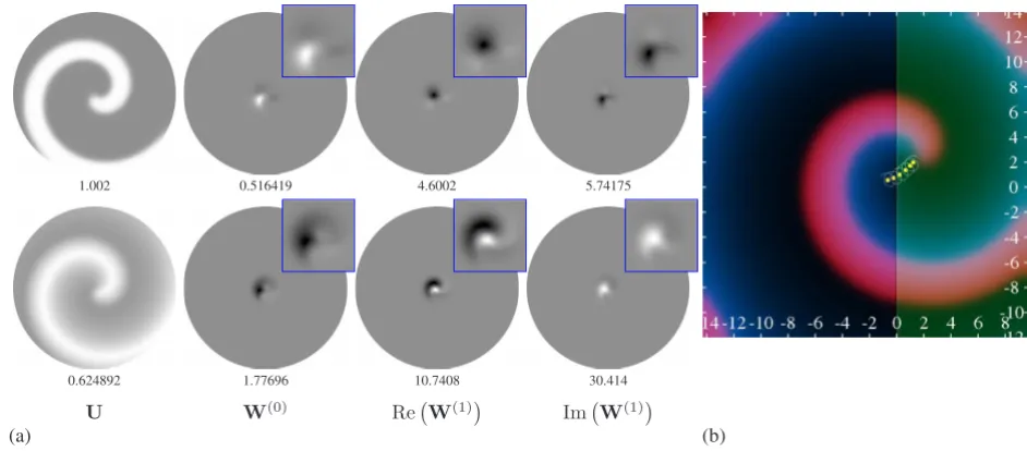
direc-tion and a varying number N_␳ of discretization intervals in the radial direction, up toN_␳= 1280. The components of the spiral wave solution and its response functions for Barkley model are shown in Fig. 1共a兲. Similar pictures for the FitzHugh-Nagumo model can be found in关47兴.

C. Perturbations

We considered similar types of perturbations⑀h共u,rជ,t兲in both FitzHugh-Nagumo and Barkley models, both for theo-retical predictions based on response functions and in nu-merical simulations. Specifically, the perturbations were taken to have the following forms.

1. Resonant drift

h共u,rជ,t兲=

冋

1

0

册

cos共␻t兲, 共43兲

where␻is the angular velocity of the unperturbed spiral obtained as part of the spiral wave solution for the Eq.共3兲.

2. Electrophoretic drift

h共u,rជ,t兲=

冋

1 0 0 0

册

⳵u

⳵x. 共44兲

3. Spatial parametric inhomogeneities

As set out in SectionII, a spatial dependence of a param-eter p of the kinetic terms in the form p共rជ兲=p₀+p₁共rជ兲, 兩p₁兩 Ⰶ兩p0兩 corresponds to the perturbation

h共u,rជ,t兲=⳵pf共u,p0兲p1共rជ兲. 共45兲

For each of the two models, we consider inhomogeneities in all three parameters, namely p苸兵␣,␤,␥其 for the FitzHugh-Nagumo model, and p苸兵a,b,c其for the Barkley model. The “linear gradient” inhomogeneity is of the form

p₁=x−x₀, 共46兲

where x0 is chosen to be in the middle of the computation box and close to the initial center rotation of the spiral wave.

The “stepwise” inhomogeneity is of the form

p1=H共x−xs兲− 1

2, 共47兲

wherexsis varied and chosen with respect to the initial cen-ter of rotation of the spiral wave. The −1₂ term is added to make the perturbation symmetric共odd兲aboutx=xs, to mini-mize the inhomogeneity impact on the spiral properties while near the step. As it can be easily seen, within the asymptotic theory, this term only affects the frequency of the spiral but not its spatial drift.

The “disk-shape” inhomogeneity is of the form

p1=H共Rin−兩rជ−rជd兩兲, 共48兲

where the position of the center of the disk rជd=共xd,yd兲T is varied and chosen with respect to the initial center of rotation of the spiral wave.

D. Drift simulations

Simulations have been performed using forward Euler timestepping on uniform Cartesian grids on square domains

1.002 0.516419 4.6002 5.74175

0.624892 1.77696 10.7408 30.414

U W(0) _ReW(1) _ImW(1)

[image:7.609.67.538.67.274.2]

(a) (b)

with nonflux boundary conditions and five-point approxima-tion of the Laplacian. The space discretizaapproxima-tion step ⌬xhas been varied between ⌬x= 0.03 and ⌬x= 0.1, and time dis-cretization step ⌬t maintained as ⌬t=1₅⌬x2_{. The tip of the} spiral is defined as the intersections of isolines u共x,y兲=u_ⴱ andv共x,y兲=v_ⴱ, and the angle ofⵜuat the tip with respect to x axis is taken as its orientation. We use共u_ⴱ,v_ⴱ兲=共0 , 0兲 for the FitzHugh-Nagumo model and共u_ⴱ,v_ⴱ兲=共1/2 ,a/2 −b兲for the Barkley model.

E. Processing the results

For coarse comparison, we use the trajectories of the in-stantaneous rotation center of the spiral wave. They are di-rectly predicted by the theory. In simulations, they are calcu-lated by averaging the position of the tip during full rotation periods, defined as the intervals when the orientation makes the full circle 共−␲,␲兴, see Fig.1共b兲.

For finer comparison, we fit the raw tip trajectories, i.e., we use theoretical predictions including the rotation of the spiral. That is, if the theory predicts a trajectory of the center as R=R共t;A,B, . . .兲苸C 共a circle for resonant drift and a straight line for electrophoretic or linear gradient inhomoge-neity drifts兲depending on parameters A,B, . . . to be identi-fied, then the trajectory of the tip is assumed in the form Rtip共t兲=R共t;A,B, . . .兲+Rcoreei共␻t+⌰0兲whereRcore苸Ris the tip rotation radius, ␻苸R is the spiral rotation frequency and ⌰0苸R is the initial phase. The parameters Rcore,␻ and⌰0 are added to the listA,B, . . . of the fitting parameters.

IV. RESULTS

A. Simple drifts

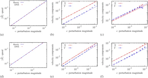
Figure2shows a comparison between the theoretical pre-dictions for the simple drifts and the results of direct numeri-cal simulations for various perturbation amplitudes ⑀. The simple drifts include the resonant drift, the electrophoretic drift and the drift in the linear parametric gradient with re-spect to one arbitrarily selected parameter.

For the resonant drift, the motion equations given by Eqs. 共18兲–共20兲 can be summarized, in terms of complex coordi-nateR=X+iY, as

dR dt =e

i⌽

p, d⌽

dt =q, 共49兲

wherep=1₂兩⑀具W共1兲_{,A典兩is predicted by the theory at leading} order, and q=O共⑀2_{兲 is not, and we only know its expected} asymptotic order. The theoretical trajectory is a circle of ra-diusp/q, and the spiral drifts along it with the speedp. In the simulations, we determined both the radius and the speed by fitting. The speed is used for comparison and the radius is ignored.

For the other two types, electrophoretic drift and linear gradient inhomogeneity drift, the theory predicts drift at a straight line, according to Eqs.共24兲and共33兲, respectively. In these cases, we measure and compare the x andy compo-nents of the drift velocities separately.

For numerical comparison in the case of linear gradient inhomogeneity, we chose pieces of trajectories not too far 10-2

10-1

10-3 10-2 10-1 theory

DNS

|

˙ _R|:

speed

: perturbation magnitude

10-3 10-2 10-1

10-3 10-2 10-1

˙ X ˙ Y

v

elocity

com

p

onents

: perturbation magnitude

10-3 10-2 10-1

10-4 10-3 10-2

˙ X ˙ Y

v

elocity

com

ponents

: perturbation magnitude

(a) (b) (c)

10-2 10-1

10-3 10-2 theory

DNS

|

˙ _R|:

speed

: perturbation magnitude

10-3 10-2 10-1

10-3 10-2 10-1

˙ X ˙ Y

v

elocity

com

p

onents

: perturbation magnitude

10-4 10-3 10-2 10-1

10-4 10-3 10-2

˙ X ˙ Y

v

elocity

com

p

onents

: perturbation magnitude

[image:8.609.65.544.68.320.2]

(d) (e) (f)

from x=x0, selected empirically to achieve a satisfactory quality of fitting.

A common feature of all graphs is that at small enough⑀, there is a good agreement between theory and simulations. As expected, differences appears for larger ⑀ with the dis-agreement occurring sooner 共for smaller values of drift speed兲 for the linear gradient inhomogeneity drift. This is related to an extra factor specific to the inhomogeneity-induced drift: the properties of the medium where they mat-ter, i.e., around the core of the spiral, change as the spiral drifts. Since we require a certain number of full rotations of the spiral for fitting, faster drift meant longer displacement along the x axis and more significant change of the spiral properties along that way, which in turn affects the accuracy of the fitting.

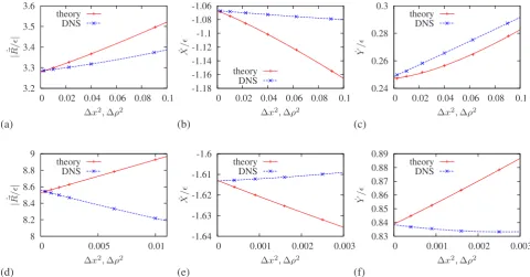
B. Numerical convergence

Figure3illustrates numerical convergence of results with discretization parameters. We consider the simple drift cases and focus on forces, defined as the drift speed/velocity per unit perturbation amplitude ⑀. The discretization parameter that primarily dictates the accuracy of solutions is a spatial discretization step: ⌬xin the simulations and the radial dis-cretization step⌬␳ in the response functions calculations.

In simulations, the forces are determined for values of⑀ well within the linear range as determined in Fig. 2. These are calculated for different values of the space discretization step ⌬x, where the time discretization changed simulta-neously so that the ratio⌬t/共⌬x兲2remains constant.

In theoretical predictions, the forces are given by the val-ues of the corresponding integrals of response functions as described by Sec. II, and we have calculated the response

functions and the corresponding integrals with various values of the radius discretization steps⌬␳.

Our discretization in both the theoretical and stimulations cases is second order in⌬xand in⌬␳, so one would expect to see linear dependence of the drift forces on the squares of these discretization steps, 共⌬x兲2 _{and 共⌬␳兲}2_{, at least for the} values of these steps small enough. This is indeed what is observed.

We have gone further and extrapolated the calculated the-oretical and simulation values of forces to zero ⌬␳ and⌬x respectively, based on the expected numerical convergence properties. Such extrapolation gives the values of the forces, which differ from the exact value only due to other, smaller discretization errors, which are: angular discretization and restriction to the finite domain in the theoretical predictions, and second-order corrections in⑀and the boundary effects in the simulations. Comparison of such extrapolated data shows a very good agreement between theory and direct numerical simulations 共DNS兲which is illustrated in Table I. Note that the values for Figs.3共e兲and3共f兲are also in good agreement with the results of 关46兴.

For the extrapolation, we fitted the numerical data with the expected numerical convergence dependencies, which were different for theoretical calculations and for the simu-lations. In simulations, the central difference approximation of the Laplacian means that the next term after 共⌬x兲2 _is 共⌬x兲4_{. The expected error due to time derivative} discretiza-tion is a power series in ⌬t⬃共⌬x兲2_{, hence, the next term} there after 共⌬x兲2is again 共⌬x兲4. The situation is different in the response functions calculations as there is no symmetry in the approximation of ␳ derivatives, therefore we expect that in the theoretical convergence, the next term after共⌬␳兲2 is共⌬␳兲3_{. We note, however, that approximation of both}

the-3.2 3.3 3.4 3.5 3.6

0 0.02 0.04 0.06 0.08 0.1 theory

DNS

|

˙ _R/

|

∆x2_,∆ρ2

-1.18 -1.16 -1.14 -1.12 -1.1 -1.08 -1.06

0 0.02 0.04 0.06 0.08 0.1 theory

DNS

˙_X/

∆x2_,∆ρ2

0.24 0.26 0.28 0.3

0 0.02 0.04 0.06 0.08 0.1 theory

DNS

˙_Y/

∆x2_,∆ρ2

(a) (b) (c)

8 8.2 8.4 8.6 8.8 9

0 0.005 0.01 theory

DNS

|

˙ _R/

|

∆x2_,∆ρ2

-1.64 -1.63 -1.62 -1.61 -1.6

0 0.001 0.002 0.003 theory

DNS

˙_X/

∆x2_,∆ρ2

0.83 0.84 0.85 0.86 0.87 0.88 0.89

0 0.001 0.002 0.003 theory

DNS

˙_Y/

∆x2_,∆ρ2

[image:9.609.64.544.67.317.2]

(d) (e) (f)

-2 -1 0 1 2 3 4

-4 -2 0 2 4

force

d: distance to step

Fx Fy

-4 -3 -2 -1 0 1 2

-4 -2 0 2 4

force

d: distance to step

Fx Fy

-2 -1.5 -1 -0.5 0 0.5 1

-4 -2 0 2 4

force

d: distance to step

Fx Fy

(a)

(b)

(c)

-4 -3 -2 -1 0 1 2 3

-4 -2 0 2 4

force

d: distance to step

Fx Fy

-20 -15 -10 -5 0 5 10 15

-4 -2 0 2 4

force

d: distance to step

Fx Fy

-150 -100 -50 0 50 100

-4 -2 0 2 4

force

d: distance to step

Fx Fy

(d)

(e)

(f)

-6 -4 -2 0 2 4

-6 -4 -2 0 2 4 theory DNS

X−xs

Y

˙

R

10-3 10-2 10-1

10-3 10-2 10-1 theory

DNS

: perturbation magnitude

˙_Y:v

er

tical

drift

sp

eed

-2 0 2

-2 0 2

theory DNS

X−xs

Y

˙

R

[image:10.609.50.555.68.622.2]

(g)

(h)

(i)

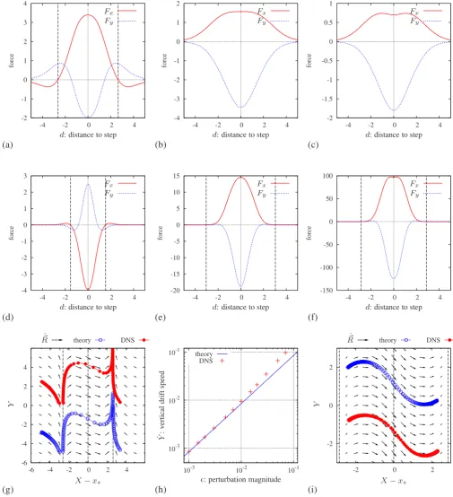
FIG. 4. 共Color online兲 Drift in stepwise inhomogeneity Eqs. 共45兲 and 共47兲. First row: theoretical predictions for the drift forces components as functions of the distance to the steps,d=X−x_s, in parameters共a兲␣,共b兲␤, and共c兲␥, in the FitzHugh-Nagumo model. Second row: same for Barkley model, steps in parameters共d兲a,共e兲band共f兲c. Third row: comparison of theoretical predictions with DNS.共g兲A phase portrait of the drift in the FitzHugh-Nagumo model, in theory, Eq.共37兲, and DNS, Eqs.共4兲,共45兲, and共47兲, with a step inhomogeneity of parameter␣关corresponds to panel共a兲兴, at⑀= 10−2. Shown are the theoretical vector field共black arrows; the lengths are nonlinearly scaled for visualization兲, a selection of theoretical trajectories共red filled circles兲and a selection of numerical trajectories共blue open circles兲of the centers of the spiral waves. Trajectories are arbitrarily shifted in the vertical direction for visual convenience. Dashed-dotted vertical lines correspond to the root of the theoretical horizontal component of the speed, and the location of the stepX−xs= 0.共h兲Speed of the established

oretical and simulation data with similar dependencies, be it with a cubic or a quartic third term, gives very similar values for the constant term: the value at infinite resolution.

C. Drift near stepwise inhomogeneity

The theoretical predictions for stepwise inhomogeneity, Eqs. 共45兲 and 共47兲 and disk-shaped inhomogeneity consid-ered next, are more complicated than the simple forms of drift considered up to this point. Because now the medium is inhomogeneous in the presence of the perturbation, the ve-locity depends on the instant position of the spiral center and as a result the spiral trajectories can be quite complex. Quali-tative comparisons between theory and simulations can be made in the general case, but for detailed quantitative com-parison we focus on the cases where the theory predicts simple attractors, e.g., a straightforward drift along the step for the stepwise inhomogeneity.

Equation 共37兲 gives a system of two first-order autono-mous differential equations for X= Re共R兲andY= Im共R兲,

X˙ =⑀Fx共X−xs兲,

共50兲 Y˙=⑀Fy共X−xs兲,

where

Fx共d兲= 1

␲

冕

0 2␲

冕

兩d兩 ⬁

Re„w共1兲共␳,␪兲e−i␪…

冑

r2−d2共d␳兲 共d␪兲, 共51兲

Fy共d兲= 1

␲

冕

0 2␲

冕

兩d兩 ⬁

Im„w共1兲共␳,␪兲e−i␪…

冑

␳2_−d2_{共d␳兲 共d␪兲.} 共52兲 The right-hand sides of system, Eqs.共50兲, depend only onX but not onY, that is, the system is symmetric with respect to translations along the Y axis. For this reason, the roots d_ⴱ:Fx共dⴱ兲= 0 provide invariant straight lines along the Y axis. An invariant line 兵共xs+d_ⴱ,Y兲兩Y苸R其 will be stable if ⑀F_x

⬘

共d_ⴱ兲⬍0 and unstable if⑀F_x

⬘

共d_ⴱ兲⬎0. Note that the stabil-ity of invariant lines reverses with a change of sign of⑀and also that Fx共d兲 is an even function. Hence, if ⑀⫽0 and dⴱ ⫽0 then either兵xs+d_ⴱ,Y其or兵xs−d_ⴱ,Y其will be an attracting invariant set.

Figures4共a兲–4共f兲show the theoretical predictions for the drift forces, i.e., velocity components per unit perturbation magnitude⑀,Fx共d兲andFy共d兲, on the distanced=X−xsfrom the instant spiral center to the step. This is done for both FitzHugh-Nagumo and Barkley models, for steps in each of the three parameters in these models. The roots ofFx共d兲are specially indicated. One can see from the given six ex-amples, that existence of roots of Fx共 兲 is quite a typical, albeit not a universal, event.

The qualitative predictions of the theory about a stable invariant line are illustrated by Fig. 4共g兲 where we present results of numerical integration of the ordinary differential equation共ODE兲 system, Eqs.共50兲, and the results of direct numerical simulation of the full system. In the example shown, the positive root d_ⴱ⬇2.644 of Fx is stable and the negative root −d_ⴱ is unstable. Hence, the theoretical predic-tion for different initial condipredic-tions are: forX共0兲⬎xs−dⴱand not too big, the spiral wave will approach the line X=xs +d_ⴱ and drift vertically along it with the speed ⑀Fy共dⴱ兲

⬇0.8468⑀; forX共0兲⬍xs−d_ⴱ, the spiral wave will drift to the left with ever decreasing speed, until its drift is no longer detectable; for big兩X共0兲兩, the drift will not be detectable from the outset.

As seen in Fig.4共g兲this is indeed what is observed, both for the theoretical and for the DNS trajectories, and the vi-sual similarity between theoretical and DNS trajectories is an illustration of the validity of the qualitative predictions of the theory.

Since the generic drift is nonstationary, a quantitative comparison for typical trajectories is difficult. However, the drift along the stable manifold X=xs+d_ⴱ is stationary with vertical velocity given by ⑀Fy共dⴱ兲so a comparison is easily made using the same methods as in the case of “simple” drifts considered in the previous subsections. The results are illustrated in Fig.4共h兲. As expected, we see good agreement between the theory and the DNS for small⑀.

The phenomenological predictions are different for the case whenFx共d兲has no roots, or when its roots are so large that 兩Fy共dⴱ兲兩 is so small that the drift cannot be detected in simulations. In such cases, the theoretical predictions for dif-ferent initial conditions are: for兩X共0兲兩not too large, the spiral wave will move with varying vertical velocity component but always in the same horizontal direction 关to the right if

⑀Fx共0兲⬎0兴, eventually with ever decreasing speed, until its drift is no longer detectable; for兩X共0兲兩too large, the drift will not be detectable from the outset.

This prediction is confirmed by simulations, as illustrated in Fig.4共i兲, where we have chosen the case of inhomogene-TABLE I. Fitting of numerical convergence of theoretical and simulation data.

Graph Theory DNS

Discrepancy 共%兲

[image:11.609.105.503.83.202.2]

ity in parametercin Barkley model, for which the smallest positive root isd_ⴱ⬇2.867, which givesFy共dⴱ兲⬇0.1632. This value should be compared to Fx共0兲⬇48.42 and Fy共0兲

⬇119.4. Note also that to get the drift velocities, FxandFy should be multiplied by ⑀ which should be much smaller than c0= 0.025. So when the spiral is further than 兩X−xs兩

⬃2 from the step, the drift is very slow and hardly notice-able. Even though according to the theory there should be stable vertical drift around X=xs+d_ⴱ, it is too slow to be observed in normal simulations.

D. Drift near disk-shape localized inhomogeneity

The theoretical predictions for the disk-shaped inhomoge-neity 关Eqs. 共45兲 and 共48兲兴, are more complicated but also more interesting. The theoretical spiral motion Eq.共41兲has a rotational, rather than the translational symmetry of the step-wise inhomogeneity. In polar coordinates 共l,␽0兲 centered at the center of the inhomogeneity, so thatR=xd+iyd+lei␽0, Eq.

共41兲can be rewritten in the form

l˙= −⑀Fr共l兲,

共53兲 l␽˙0=⑀Fa共l兲,

whereFrandFaare the radial and azimuthal components of the drift force, given by

Fr=

冕

0

2␲

冕

兩l−R_in兩 l+R_in

Re„w共1兲共␳,␪兲e−i␪…

⫻

冑

1 −

冉

␳

2_+l2_−R in 2

2l␳

冊

2

␳d␳d␪, 共54兲

Fa=

冕

0

2␲

冕

兩l−R_in兩 l+R_in

Im„w共1兲共␳,␪兲e−i␪…

⫻

冑

1 −

冉

␳

2_+l2_−R in 2

2l␳

冊

2

␳d␳d␪. 共55兲

The minus sign in the first equation of Eqs.共53兲comes from the fact that in Eq.共41兲, the origin was placed at the instant rotation center of the spiral, and the position of inhomoge-neity is determined with respect to it, where as now we do the other way round: the origin is at the center of inhomoge-neity and the current position of the spiral rotation center is determined with respect to it.

In Eqs.共53兲, the axial symmetry is manifested by the fact that the right-hand sides of Eqs.共53兲depend onlbut not on

␽0, and the equation forl is a closed one. Hence rootslⴱof Fr共lⴱ兲= 0 represent invariant sets, which in this case are cir-cular orbits. The movement along those orbits will have a linear speed ⑀Fa共l_ⴱ兲 and angular speed ⍀=⑀Fa共l_ⴱ兲/l_ⴱ. The stability of these orbits is determined by the sign of⑀Fr

⬘

共lⴱ兲: stable for positive and unstable for negative. Unlike the case of the stepwise inhomogeneity, now we do not have any mirror symmetries, as only positive l make sense, therefore for a given rootl_ⴱa stable circular orbit is guaranteed only for one sign of ⑀but not the other.

Figures5共a兲–5共f兲 show the theoretical predictions for the drift forces Fr共l兲 andFa共l兲. This is done for both FitzHugh-Nagumo and Barkley models, for inhomogeneities in each of the three parameters in these models. The roots ofFr共l兲are specially indicated. One can see from the six given examples that existence of roots of Fr共 兲 is rather common and often there is more than one root,lj, such that 0 =l0⬍l1⬍l2⬍. . .. The qualitative predictions of the theory are illustrated in Figs. 5共h兲 and 5共i兲 where we present results of numerical integration of the ODE system, Eqs.共53兲, and the results of direct numerical simulations of the full system. In the ex-ample shown in Fig. 5共h兲, the predictions are given by Fig.

5共e兲, which say that the smallest orbit has radius l1⬇3.724, with the orbital speed Fa共l1兲⬇0.003938, which is rather small compared to max共兩Fr共l兲兩兲⬇3.458 and max共兩Fa共l兲兩兲

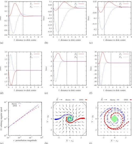
⬇8.534 and hardly observable in numerical simulations. Hence, in this case, the radial component of the drift speed Fr共l兲 is effectively constant sign, and for negative ⑀, one should observe repulsion of the spiral wave from the inho-mogeneity until it is sufficiently far from it, l⬃3, to stop feeling it, and for positive⑀, the spiral wave will be attracted toward the center of inhomogeneity from any initial position l⯝3. This is indeed what is observed in simulations shown in Fig.5共h兲where the case of⑀⬎0 is shown, and the center of the inhomogeneity, l=l0, is attracting for the spiral wave. In the example shown in Fig.5共i兲, the inhomogeneity cen-ter l0= 0 is repelling. Instead, the first orbit of radius l1 ⬇1.7722 is attracting. The perturbation amplitude⑀= 0.3 in this case is quite large and comparable with the value ␥₀ = 0.5 of the perturbed parameter itself. We see that although the numerical correspondence between theory and DNS in this case is not very good 共note the distances between the open circles and between the filled circles兲, the qualitative prediction of orbital movement remains impeccable. As ex-pected, the numerical correspondence becomes good for smaller values of⑀, see Fig.5共g兲.

V. DISCUSSION

We have considered symmetry-breaking perturbations of three different kinds: time-translation symmetry breaking that is homogeneous in space and periodic in time共“resonant drift”兲; rotational symmetry breaking through differential ad-vective terms共“electrophoretic drift”兲; and spatial translation symmetry breaking through space-dependent inhomogene-ities 共“inhomogeneity induced drift”兲. The latter type in-cludes three subcases: a linear parametric gradient, a step-wise parameter between two half- planes, and a parameter inhomogeneity localized within a disk.

A. Quantitative: drift velocity

-0.8 -0.6 -0.4 -0.2 0 0.2 0.4 0.6

0 1 2 3 4 5 6 7 8 9

force

l: distance to disk centre

Fr Fa

-0.4 -0.35 -0.3 -0.25 -0.2 -0.15 -0.1 -0.05 0 0.05 0.1

0 1 2 3 4 5 6 7 8 9

force

l: distance to disk centre

Fr Fa

-0.25 -0.2 -0.15 -0.1 -0.05 0 0.05

0 1 2 3 4 5 6 7 8 9

force

l: distance to disk centre

Fr Fa

(a)

(b)

(c)

-2 -1.5 -1 -0.5 0 0.5 1 1.5 2 2.5

0 1 2 3 4 5 6 7 8 9

force

l: distance to disk centre

Fr Fa

-10 -8 -6 -4 -2 0 2 4

0 1 2 3 4 5 6 7 8 9

force

l: distance to disk centre

Fr Fa

-60 -50 -40 -30 -20 -10 0 10 20 30

0 1 2 3 4 5 6 7 8 9

force

l: distance to disk centre

Fr Fa

(d)

(e)

(f)

10-5 10-4 10-3 10-2 10-1

10-3 10-2 10-1 100 theory

DNS

: perturbation magnitude

Ω

:

o

rbiting

angular

sp

eed

-2 0 2

-2 0 2

theory DNS

X−xd

Y

−

yd

˙

R

-2 0 2

-2 0 2

theory DNS

X−xd

Y

−

yd

˙

R

[image:13.609.55.556.66.614.2]

(g)

(h)

(i)

FIG. 5.共Color online兲Drift around disk-shape inhomogeneity Eqs.共45兲and共48兲of radiusR_in= 0.56. First row: theoretical predictions for the drift speed components as functions of the distance to the disk center,l=共共X−xd兲2+共Y−yd兲2兲1/2, for inhomogeneity in parameters共a兲␣,

B. Qualitative: attachment and orbiting

In the more complicated cases of spatial inhomogeneity, the response functions allow us to predict qualitatively dif-ferent regimes of spiral motion, which we have been able to confirm by direct simulations. In the presence of a stepwise inhomogeneity, the center of spiral wave rotation may either be attracted to one side of the step where it gradually “freezes,” or it may get attached to the step and drift along it with the constant velocity. In the latter case, the speed of the drift is proportional to the inhomogeneity strength, whereas the distance at which the attachment happens, does not de-pend on the inhomogeneity strength at leading order. If the sign of inhomogeneity is inverted, the attachment occurs on the opposite side of the step and proceeds in the opposite direction.

In disk-shape inhomogeneity, the situation is somewhat similar but more interesting. The spiral wave may be at-tracted toward the center of the disk, or repelled from it. It may also be attracted to or repelled from one or more circu-lar orbits. The drift velocity along the orbits is proportional to the strength of the inhomogeneity, whereas the radii of orbits do not depend on it at leading order. The repulsion changes to attraction and vice versa, with the change of the sign of the inhomogeneity.

C. Prevalence of attachment and orbiting

The possibilities of attachment to the step inhomogeneity and orbital movement for the disk-shape inhomogeneity are both related to the change of sign of the integrals of the translational response functions, which in turn are possible due to changes of sign of the components of those response functions. Not surprisingly, there is a certain correlation be-tween these phenomena. The graphs Figs. 5共a兲–5共f兲may be viewed as deformed versions of the corresponding graphs Figs.4共a兲–4共f兲. Respectively, positive roots ofFx共d兲in Figs. 4共a兲and4共d兲–4共f兲have corresponding roots ofFr共l兲in Figs. 5共a兲 and5共d兲–5共f兲. However, the integrals in Eqs. 共51兲 and 共54兲are only similar but not identical, and the above corre-spondence between the roots is not absolute: the roots of Fr共l兲 in Figs. 5共b兲 and 5共c兲 and the smaller roots of this function in Figs. 5共a兲 and5共f兲 have no correspondences in Fig. 4. Overall, based on results considered, orbital motion around a localized inhomogeneity seems to be more preva-lent than attachment to a stepwise inhomogeneity. Moreover, the typical situation seems to be that there are multiple sta-tionary orbits around a disk inhomogeneity. We have already discussed this situation in our recent short communication 关52兴 where we have also illustrated how for the initial con-ditions between two stationary orbits, the spiral wave launched into one orbit or the other depending on the sign of the inhomogeneity.

The possibility of orbital drift, related to a change of sign of an equivalent to the functionFr共l兲, has been discussed at a speculative level in 关53兴. The sign change of translational response functions was observed in oscillatory media de-scribed by CGLE 关54,55兴. The examples we consider here suggest that this theoretical possibility is in fact quite often realized in excitable media, and even multiple orbits are

quite typical. Theoretical reasons for this prevalence are not clear at present. As stated in关52兴, the prevalence of multiple orbits may be understood in terms of asymptotic theories involving further small parameters. So, the version of kine-matic theory of spiral waves suggested in关56兴 produces an equivalent of response functions, which is not only quickly decaying, but also periodically changing sign at large radii, with an asymptotic period equal to the quarter of the asymptotic wavelength of the spiral wave. Other variants of the kinematic theory, e.g., 关57,58兴 did not reveal any such features on a theoretical level. However, numerical simula-tions of kinematic equasimula-tions presented in 关57兴 showed at-tachment of spiral waves to nonflux boundaries, which in a sense is similar to attachment to stepwise inhomogeneity. On a phenomenogical level, such attachment is, of course well known since the earliest simulations of excitable media, e.g., 关38兴.

D. Orbiting drift vs other spiral wave dynamics

Properties of the orbital drift resemble properties of reso-nant drift when the stimulation frequency is not fixed as in the examples above, but is controlled by feed-back 关59兴. In that case, the dynamics of the spiral wave is controlled by a closed autonomous system of two differential equations for the instant center of rotation of the spiral, like Eqs. 共50兲or Eqs. 共53兲. In particular, depending on the detail of the feed-back, this planar system may have limit cycle attractors, dubbed “resonant attractors” in关60兴, which may have circu-lar shape if the system with the feedback has an axial sym-metry. Apart from this being a completely different type of drift, we also comment that the second order ODE system is an approximation subject to the assumption that the feedback is instant, and in the situations when the delay in the feed-back is significant due to the system size and large distance between spiral core and feedback electrode, the behavior be-comes more complicated.

For some combination of parameters, the trajectory of an orbiting spiral may also resemble meandering and may be taken for this in simulations or experiments. So, it is possible that orbital movement was actually observed by Zou et al. 共关61兴, p.802兲 where they reported spiral “meandering” around a “partially excitable defect;” although it is difficult to be certain as no details are given. The difference is that spiral meandering, in the proper sense, is due to internal instabilities of a spiral wave, whereas orbital motion is due to inhomogeneity. E.g. in orbiting, the “meandering pattern” determined by ⍀/␻ will change depending on the inhomo-geneity strength.

phe-nomenon may be observed in strong inhomogeneities as well. This offers an unexpected aspect on the problem of pinning. Instead of a simplistic “binary” viewpoint, that a local inhomogeneity can either be attractive, which is the case of pinning, or repelling, which is the case of unpinning, there is actually a third possibility, which can in fact be more prevalent than the first two, namely, that at some initial con-ditions the spiral may orbit around one of a number of cir-cular orbits, regardless of whether or not it is attracted to the center, which can be considered just as one of the orbits that happens to have radius zero. That is, there is more than one way that a spiral may be bound to inhomogeneities.

VI. CONCLUSION

We have demonstrated that the asymptotic theory of spiral wave drift in response to small perturbations, presented in 关36,45兴, works well for excitable media, described by FitzHugh-Nagumo and Barkley kinetics models and gives accurate quantitative prediction of the drift for a wide selec-tion of perturbaselec-tions. The key objects of the asymptotic theory are the response functions, i.e., the critical eigenfunc-tions of the adjoint linearized operator. The RFs have been found to be localized in most models where they have been calculated; however there are counterexamples demonstrat-ing that surprises are possible 关66兴. Physical intuition tells that for the response function to be localized, the spiral wave

should be indifferent to distant perturbations, which will be the case if the core of the spiral is a “source” rather than a “sink” in the sense of the flow of causality, for example as defined by the group velocity. Indeed, this localization prop-erty has been proven for one-dimensional analogs of spiral waves关67兴and there is hope that this result can be extended to spiral and scroll waves.

The effective spatial localization of the RFs on the math-ematical level guarantees convergence of the integrals in-volved in asymptotic theory, and on the physical level ex-plains why wave-like objects such as spiral and scroll waves, while stretching to infinity and synchronizing the whole me-dium, behave respectively as particlelike and stringlike local-ized objects. This macroscopic dissipative wave-particle du-ality of the spiral waves has been previously demonstrated for the complex Ginzburg-Landau equation关45兴which is the archetypical oscillatory media model. Here, we confirmed it for the most popular excitable media models important for many applications.

ACKNOWLEDGMENTS

This study has been supported in part by EPSRC共Grants No. EP/D074789/1 and No. EP/D074746/1兲. D.B. also grate-fully acknowledges support from the Leverhulme Trust and the Royal Society.

关1兴T. Frisch, S. Rica, P. Coullet, and J. M. Gilli,Phys. Rev. Lett. 72, 1471共1994兲.

关2兴B. F. Madore and W. L. Freedman, Am. Sci. 75, 252共1987兲. 关3兴L. S. Schulman and P. E. Seiden,Science 233, 425共1986兲. 关4兴A. M. Zhabotinsky and A. N. Zaikin, inOscillatory Processes

in Biological and Chemical Systems, edited by E. E. Selkov, A. A. Zhabotinsky, and S. E. Shnol共Nauka, Pushchino, 1971兲, p. 279.

关5兴S. Jakubith, H. H. Rotermund, W. Engel, A. von Oertzen, and G. Ertl,Phys. Rev. Lett. 65, 3013共1990兲.

关6兴M. A. Allessie, F. I. M. Bonke, and F. J. G. Schopman, Circ. Res. 33, 54共1973兲.

关7兴N. A. Gorelova and J. Bures,J. Neurobiol. 14, 353共1983兲. 关8兴F. Alcantara and M. Monk,J. Gen. Microbiol. 85, 321共1974兲. 关9兴J. Lechleiter, S. Girard, E. Peralta, and D. Clapham, Science

252, 123共1991兲.

关10兴A. B. Carey, R. H. Giles, Jr., and R. G. McLean, Am. J. Trop. Med. Hyg. 27, 573共1978兲.

关11兴J. D. Murray, E. A. Stanley, and D. L. Brown,Proc. R. Soc. London, Ser. B 229, 111共1986兲.

关12兴A. G. Shagalov,Phys. Lett. A 235, 643共1997兲.

关13兴P. Oswald and A. Dequidt,Phys. Rev. E 77, 051706共2008兲. 关14兴Ye. Larionova, O. Egorov, E. Cabrera-Granado, and A.

Esteban-Martin,Phys. Rev. A 72, 033825共2005兲.

关15兴D. J. Yu, W. P. Lu, and R. G. Harrison, J. Opt. B: Quantum Semiclassical Opt. 1, 25共1999兲.

关16兴K. Agladze and O. Steinbock, J. Phys. Chem. A 104, 9816

共2000兲.

关17兴T. Bretschneider, K. Anderson, M. Ecke, A.

Müller-Taubenberger, B. Schroth-Diez, H. C. Ishikawa-Ankerhold, and G. Gerisch,Biophys. J. 96, 2888共2009兲.

关18兴M. A. Dahlem and S. C. Müller,Biol. Cybern. 88, 419共2003兲. 关19兴O. A. Igoshin, R. Welch, D. Kaiser, and G. Oster,Proc. Natl.

Acad. Sci. U.S.A. 101, 4256共2004兲.

关20兴K. I. Agladze, V. A. Davydov, and A. S. Mikhailov, JETP Lett. 45, 601共1987兲.

关21兴K. I. Agladze and P. Dekepper, J. Phys. Chem. 96, 5239

共1992兲.

关22兴V. G. Fast and A. M. Pertsov,J. Cardiovasc. Electrophysiol.3, 255共1992兲.

关23兴J. M. Davidenko, A. M. Pertsov, R. Salamonsz, W. Baxter, and J. Jalife,Nature共London兲 355, 349共1992兲.

关24兴M. Markus, Z. Nagy-Ungvarai, and B. Hess,Science 257, 225

共1992兲.

关25兴C. Luengviriya, U. Storb, M. J. B. Hauser, and S. C. Müller, Phys. Chem. Chem. Phys. 8, 1425共2006兲.

关26兴S. Nettesheim, A. von Oertzen, H. H. Rotermund, and G. Ertl, J. Chem. Phys. 98, 9977共1993兲.

关27兴A. M. Pertsov, J. M. Davidenko, R. Salomonsz, W. T. Baxter, and J. Jalife, Circ. Res. 72, 631共1993兲.

关28兴Z. Y. Lim, B. Maskara, F. Aguel, R. Emokpae, and L. Tung, Circulation 114, 2113共2006兲.

关29兴S. Lugomer, Y. Fukumoto, B. Farkas, T. Szörényi, and A. Toth, Phys. Rev. E 76, 016305共2007兲.

关30兴L. V. Yakushevich, Stud. Biophys. 100, 195共1984兲.

关31兴A. M. Pertsov and E. A. Ermakova, Biophys. 33, 364共1988兲. 关32兴M. Wellner, A. M. Pertsov, and J. Jalife, Phys. Rev. E 59,