Coarsening dynamics in a two species zero range process

University of Warwick institutional repository: http://go.warwick.ac.uk/wrap

This paper is made available online in accordance with

publisher policies. Please scroll down to view the document

itself. Please refer to the repository record for this item and our

policy information available from the repository home page for

further information.

To see the final version of this paper please visit the publisher’s website.

Access to the published version may require a subscription.

Author(s): RS. Großkinsky and T. Hanney

Article Title: Coarsening dynamics in a two-species zero-range process

Year of publication: 2005

Link to published article:

arXiv:cond-mat/0412593v2 [cond-mat.stat-mech] 9 Aug 2005

S. Großkinsky1 _{and T. Hanney}2

1 _{Zentrum Mathematik, Technische Universit¨at M¨unchen, 85747 Garching bei M¨unchen, Germany} 2 _{School of Physics, University of Edinburgh, Mayfield Road, Edinburgh, EH9 3JZ, United Kingdom}

We consider a zero-range process with two species of interacting particles. The steady state phase diagram of this model shows a variety of condensate phases in which a single site contains a finite fraction of all the particles in the system. Starting from a homogeneous initial distribution, we study the coarsening dynamics in each of these condensate phases, which is expected to follow a scaling law. Random walk arguments are used to predict the coarsening exponents in each condensate phase. They are shown to depend on the form of the hop rates and on the symmetry of the hopping dynamics. The analytic predictions are found to be in good agreement with the results of Monte Carlo simulations.

I. INTRODUCTION

Since the first observation of a condensation transition in the homogeneous zero-range process (ZRP) [1] there has been a lot of activity to further study this phenomenon on the level of the steady state [2], and on the level of the relaxation dynamics [2, 3]. When the density of particles exceeds a critical value, the system has been shown to phase separate into a homogeneous background and a condensate which contains a finite fraction of all the particles in the system. In the steady state the condensate occupies only a single lattice site, and starting with homogeneous initial conditions, the relaxation dynamics exhibit an interesting coarsening phenomenon.

Besides being of interest in its own right as an example of a condensation transition in an exactly solvable model, the phenomenon is relevant in a more general context, providing a criterion for phase separation in driven diffusive systems [4, 5]. The basic condensation mechanism is by now well understood on a static and dynamic level, but generalizations continue to be a topic of current interest, such as coarsening behaviour on scale-free networks [6], processes with defect sites [7] or applications to bipartite graphs [8]. Of particular interest are generalisations to two-species zero-range processes with two conservation laws, which also exhibit condensation and have a much richer stationary phase diagram than that of the single species system [9, 10]. Indeed, while the stationary and dynamical properties of one-dimensional driven diffusive systems with one species of particles are relatively well understood, much less is known about the properties, and in particular the dynamical properties, of driven systems with two or more species of conserved particles (see [11] for a recent review).

This paper provides a first analysis of the coarsening dynamics of a two-species zero-range process. We generalize the arguments in [2] for a single species system, which turns out to be far from straightforward since several new effects have to be taken into account, effects due to the coupled dynamics of the two particle species. The model is chosen such that all the expected new features can be observed while the steady state is exactly solvable. In addition to this theoretical interest, the results are relevant for physical realisations of two species zero-range processes, which can be found for example in shaken bidisperse granular systems [12] and models of directed networks [13].

In Section II, we define the model which is a generalisation of the model considered in [10], recap some known results for the steady state and give the phase diagram. In Section III we state the expected scaling behaviour for the coarsening regime and explain the random walk arguments for its analysis. The main results of the paper are derived in Section IV: scaling laws for the time evolution of the mean condensate size for all regions of the phase diagram, generalizing the derivation in [2]. The predictions are compared to Monte Carlo simulation data and we find good agreement. We conclude in Section V and include a discussion of finite size effects in an appendix.

II. MODEL

A. Definition and steady state

We define the two-species zero-range process on a one-dimensional lattice containingLsites with periodic boundary conditions. On this lattice, there areN1 particles of species 1 andN2 particles of species 2. A site with occupation

numbers k1 and k2 for species 1 and 2 respectively, loses a particle of species 1 with rateg1(k1, k2) and of species 2

with rateg2(k1, k2). For simplicity we assume that particles hop to their nearest neighbour site to the right, although

our results also apply for more general hopping of finite range.

The steady states for this model with general g1(k1, k2) and g2(k1, k2) have been characterised in [9, 14] and we

probabilities assume a factorised form

νL

z(k) =

L

Y

x=1

νz(k1,x, k2,x), (1)

provided the hop rates satisfy the constraint

g1(k1, k2)

g1(k1, k2−1)

= g2(k1, k2)

g2(k1−1, k2)

, (2)

for allk1, k2≥1. The single-site distribution has the form

νz(k1, k2) =

1

Z(z)f(k1, k2)z

k1

1 z2k2 , (3)

wheref(k1, k2) is a stationary weight which can be written

f(k1, k2) =

k1

Y

i=1

1

g1(i,0)

k2

Y

j=1

1

g2(k1, j)

. (4)

Herez= (z1, z2),zi ≥0 play the role of fugacities for each species, in that they are chosen to fix the particle densities ρi = hNiiν/L for species i = 1,2, i.e. the expected number of particles per site in the steady state. Thus we are

working in a grand canonical ensemble, which is normalised by the single site partition function Z(z). This steady state can be directly obtained by substitution into the balance condition for the steady state probability that the system is in a configurationk.

We remark that one gets the same steady state if the hopping dynamics are symmetric, rather than asymmetric as defined above. A useful property of the steady state [9, 14] is that the expectation value of the hop rate of speciesi, denoted byhgiiν, is equal tozi. Thushgiiν is a translation invariant quantity; this is obvious in the case of asymmetric

dynamics wherehgiiν is the current, but less obvious in the case of symmetric dynamics with vanishing current, where

hgiiν>0.

We are interested in the coarsening dynamics of the model in various phases that arise for a particular choice of rates, namely

g1(k1, k2) =

1 +b/(k1+ 1)γ

1 +b/k1γ

k2

(1 +c/k1),

g2(k1, k2) = 1 +b/(k1+ 1)γ , (5)

whereg1(0, k2) =g2(k1,0) = 0 andb, c, γ >0. It is easy to check by substitution that these rates satisfy the constraint

(2). The stationary weights, obtained from (4), are given by

f(k1, k2) =

k1!

(1 +c)k1

1 + b (k1+ 1)γ

−k2

, (6)

where (a)k=Qk −1

i=0(a+i) is the Pochhammer symbol. The single-site partition function is given by

Z(z) =

∞

X

k1,k2=0

f(k1, k2)z1k1z

k2

2 =

∞

X

k1=0

zk1

1

(k1+ 1)γ+b

(1−z2)(k1+ 1)γ+b

k1!

(1 +c)k1

. (7)

We make the choice (5) in order to study the behaviour when the dynamics of one of the particle species, here species 2, depends only on the number of particles of the other species at the departure site. So condensation of species 2, when it occurs, is induced by the presence of species 1 particles, which can be interpreted as an evolving disordered background as discussed for a specific case in Section IV.C. Thek2 dependence in g1 is then determined

by the constraint (2). The second factor (1 +c/k1) in g1 could be replaced by any function ofk1 and the steady

state will still factorise. The form we have chosen is the simplest form of the hop rate for which the single-species zero-range process exhibits a condensation transition for c >2 at a finite critical density of particles [1]. Thus the parameterccan be tuned to allow also condensation of species 1 particles, which influences the phase diagram of the process as discussed in Section II.B. We remark that the existence of condensation transitions and any subsequent coarsening behaviour depend only on the asymptotic forms of the rates. Other choices of this second factor, with different asymptotic properties, lead either to no transition of species 1 particles if it is non-decreasing or tends to a constant faster than 2/k1 as k1 → ∞, or to condensation at any density (where the fraction of particles in the

condensate is equal to one) if it tends to zero as k1 → ∞. Thus (5) are basic rates which capture two different

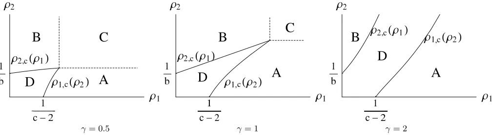
γ= 0.5 γ= 1 γ= 2

FIG. 1: Phase diagram for the choice of rates (5) with b = 1, c = 4 and several values ofγ. For γ = 0.5 and γ = 1 it is

c >max(2 +γ,1 + 2γ) and region C exists. Whereas forγ = 2 we havec <max(2 +γ,1 + 2γ) and region C does not exist. See text for details.

B. Stationary phase diagram

The range of possible fugacities is given by the domain of convergence of the partition functionZ(z) given in (7). In the present case the maximal fugacities arez1= 1 andz2= 1 and when one or both of the fugacities are maximal we

use the notationz=zc. The phase diagram in terms of the particle densitiesρ1andρ2 has been derived in [10, 15].

For the grand canonical ensemble (3) the densities are given by

ρi=zi

∂lnZ(z)

∂zi

, i= 1,2 , (8)

and thus the convergence properties of the partition function at the maximal fugacities determine whether or not the critical densities ρi,c := ρi_z

i=1 are finite or infinite. In general, ρ1,c can depend on ρ2 i.e. ρ1,c =ρ1,c(ρ2) and vice

versa. Ifρi≤ρi,cfori= 1,2, both species are in a fluid phase corresponding to a factorised steady stateνz as given

in (3). In the phase diagram shown in Figure 1 this region is denoted by D. If the particle densityρi of either species i= 1,2 exceeds its critical valueρi,c, speciesicondenses: the system phase separates into a homogeneous background

fluid phase with distributionνzc, and a condensate which contains the (ρi−ρi,c)L‘excess’ particles of speciesi. In a

typical stationary configuration this condensate occupies a single, randomly located site.

Depending on the values ofcandγ in (5) the following phases appear in the phase diagram in addition to the fluid phase D:

• In region A, the fugacities are zc = (1, z2) with z2 < 1. The species 1 particles condense and the species 2

particles form a fluid. The particle densities in the background phase are (ρ1,c, ρ2).

• In region B, the fugacities are zc = (z1,1) with z1 < 1, species 2 condenses and the background particle

densities are (ρ1, ρ2,c). As an additional point, the site containing the condensate of species 2 particles also

containsO(L1/(1+γ)_{) species 1 particles [9].}

• In region C, zc = (1,1). A single site contains condensates of both species and the background densities are

(ρ1,c, ρ2,c).

The phase diagram shown in Figure 1 is richest when c >max(2 +γ,1 + 2γ), where all three regions are found. For 2< c≤max(2 +γ,1 + 2γ) the phase diagram contains only the phases A, B and D, and forc≤2 only phases B and D remain.

So far we have discussed straightforward generalisations of previously known results. We now turn to the main aim of this work, which is to study the coarsening dynamics of the two-species zero-range process leading to each of the condensate phases A, B and C.

III. COARSENING

In the following we use the symbol≈to denote asymptotic expansions in the thermodynamic limit L → ∞with fixed particle densities, i.e.N1= [ρ1L] andN2= [ρ2L]. If the terms in the expansion are only given up to a constant

A. Relaxation dynamics

In this section we outline the arguments used to describe the coarsening dynamics in the condensate phases. Starting from an initially uniform distribution of particles, the dynamics of the condensation can be divided into three regimes: (i) nucleation, during which excess particles of either species accumulate at several randomly located sites, which we call cluster sites. Each contains O(L) particles, so there are O(1) cluster sites, separated by a typical distance of order L. At the remaining sites, which we callbulk sites, the system relaxes to its steady state distributionνzc.

(ii) coarsening, during which the cluster sites exchange particles through the bulk. This leads to the growth of large condensates at the expense of smaller ones and a decrease in the number of cluster sites.

(iii) saturation, where eventually only two cluster sites remain due to the finite size of the system. In this regime the dynamics, under which the system reaches a typical steady state configuration with a single cluster site, is different from the coarsening dynamics (cf. [2]).

Physically, the most interesting is the coarsening regime. Here, large condensates gain particles at the expense of smaller ones which causes some condensates to disappear. This in turn leads to a decrease in the number of cluster sites and hence an increase of the mean condensate size mi(t), defined as the number of particles of speciesi= 1,2

at cluster sites divided by the number of cluster sites at time t. In the limit t→ ∞, mi(t) converges to its steady

state value (ρi−ρi,c)L, the number of excess particles of speciesi in the system. Within the coarsening regime the

increase of the mean condensate size is expected to follow a scaling law,

mi(t)_L∼tβi. Moreover, on a certain time

scaleτ =τ(L), the growth of the normalised mean condensate size is expected to be independent of the system size

L,

mi(t)_L

(ρi−ρi,c)L

∼(t/τ)βi _{. (9)}

Therefore the scaleLof the mean condensate size and the time scaleτare connected viaL∼τβi_{, and thusτ ∼L}1/βi_.

The angled brackets h..iL denote an ensemble average in a finite system of size L, starting with a homogeneous

distribution of Nj = [ρjL] particles for both species j = 1,2. This is in contrast to the steady state expectation

denoted byh..iν. The scaling law (9) defines the exponentβi, which may depend on the particle speciesi. In general

one could choose different observables to monitor the coarsening process, such as the square sum of occupation numbers. But in our case the mean condensate size is a natural choice, since it is directly accessible by our arguments given below.

We remark that the scaling law (9) is of the same form as that which describes the growth of characteristic length scales in phase ordering dynamics [16]. More precisely one can define a scaling function

hi(t ′

) := lim

L→∞

mi(t′τ)_L

(ρi−ρi,c)L

, (10)

for allt′

≥0. With the appropriate time scaleτ, which will be derived in the next section for the various phases,hi

is expected to be a non-degenerate, smoothly increasing function with the asymptotic properties

hi(t′) =O t′βi fort′→0 and lim t′→∞hi(t

′

) = 1. (11)

So for smallt′

the coarsening regime is described by a power law (9) which we study in the following. Fort′

→ ∞the

system saturates and hi converges to its maximal value 1. We do not further discuss the behaviour in this regime,

this has been done for a single species system in [2].

B. Random walk arguments

In the following, our aim is to estimate the exponentsβi in each of the condensate phases A, B and C of the model

(A1) Separation of time scales:

The nucleation process is very fast so that during the coarsening regime the bulk sites have already relaxed to the steady state distributionνzc.

Within the coarsening regime the system can therefore be separated into a stationary bulk and a finite number of isolated cluster sites. On top of stationary hop rateshgiiν =zi,c, cluster sites of species iexchange particles through

the bulk on a slower time scale, given below. The bulk can be seen as a homogeneous medium through which these excess particles perform a biased random walk, and the cluster sites as boundaries where they enter and exit. (A2) Independence of excess particles in the bulk:

The excess particles exchanged by cluster sites perform independent (biased) random walks through the bulk on their way to the next cluster site and do not effect the bulk distributionνzc.

This is justified below by noting that the average density of excess particles in the bulk vanishes forL→ ∞.

The random walk argument then proceeds as follows. We consider the case where one speciesi= 1 or 2 condenses. The rates we consider decay asgi−1∼k

−α

i with 0< α≤1 (see Section IV) and the average hop rate in the bulk is zi,c = 1. So the effective rate at which cluster sites withki ∼L lose particles to the bulk isgi−zi,c∼L−α. These

excess particles perform a biased random walk through the bulk with drift

hgi|ki>0iν− hgiiν=

hgiiν

1−νzc(ki= 0)

− hgiiν =

1 1−νzc(ki= 0)

−1 . (12)

Since νzc(ki = 0) > 0 this is positive and independent ofL. Thus the time it takes an excess particle to reach a

neighbouring cluster site scales as the typical distance between cluster sites which isO(L). Sonindependent excess particles exit the bulk with rate O(n/L) which has to balance the entry rate of order L−α_{. Hence, the number of}

excess particles in the bulk scales as O(L1−α_{) which grows only sublinearly with L for 0 < α≤1, consistent with}

(A2).

In this balanced situation the time scale on which cluster sites exchange single particles through the bulk isO(Lα_).

The time scale on which cluster sites exchange a finite fraction ∼ L of their particles is thus O(L1+α_{). Since by}

definition the number of cluster sites during coarsening is of order 1, this sets the coarsening time scaleτ and the coarsening exponentβi in (9) to be

τ ∼L1+α, βi= 1

1 +α . (13)

With the above considerations we can give an additional motivation for the scaling behaviour (9). We have seen that the rate at which cluster sites exchange particles through the bulk depends on their size ask−α

i . Thus, in a very rough

approximation, the time derivative of the average condensate size

mi(t)_L should be proportional to the average

exchange rate of excess particles,

d

mi(t)_L dt ∼

mi(t) −α

L . (14)

As the solution we recover the scaling law (9) with exponentβias given above. This is of course not a strict argument

and should not be understood as a derivation of the scaling law.

Compared to the bulk dynamics the coarsening is a very slow process and typical configurations with cluster sites on top of a stationary background are quasi-stationary, i.e. within times of order 1 the configurations at cluster sites do not change on average. To leading order inLthe dynamics on cluster sites have to be compatible with the stationary bulk dynamics. By compatibility we mean that the translation invariance ofhgiiν implies that it must be the same

for all sites (both cluster sites and bulk sites) in the system. For two-component systems, this induces consistency relations between the occupation numbers k1 and k2 on cluster sites, a fact that will often be used below. If these

relations are not fulfilled, the configuration is not quasi-stationary in the above sense and changes on time scales of order 1 through interaction with the bulk.

IV. COARSENING SCALING LAWS A. Theoretical predictions

1. Phase A

In phase A,ρ1> ρ1,cand only the first species condenses. There are (ρ1−ρ1,c)Lexcess particles of species 1 in the

system and at the cluster sitesk1=O (ρ1−ρ1,c)L, whilek2 remains finite in the limitL→ ∞, which is justified

below by compatibility with the bulk. Hence, at the cluster sites the rates (5), up to first order ink1, are given by

g1(k1, k2)≈1 +c/k1, g2(k1, k2)≈1 +b/kγ1 . (15)

Thus the coarsening of the species 1 particles is independent of the second species: the net rate at which particles leave a cluster site is g1−1 = c/k1. Following the arguments leading to (13) in Section III.B the coarsening time

scale is thus

τA∼[(ρ1−ρ1,c)L]2, (16)

and we expect that the normalised mean condensate size grows like hm1(t)iL

(ρ1−ρ1,c)L

∼(t/τA)1/2 i.e. β1= 1/2. (17)

This recovers the known coarsening of the condensate in the one-species ZRP where particles hop with rate 1 +c/k

[2, 3].

Further, because the jump rates of both species are coupled, the presence of a species 1 condensate influences the distributionP of the species 2 particles on the cluster site: Since cluster sites and bulk have to be compatible,g2on

the cluster site has to be equal to the bulk steady state currenthg2iν=z2<1, and using (15) we have

hg2iν ≈(1 +b/kγ1)P(k2>0) ≈ P(k2>0). (18)

ThereforeP(k2= 0)≈1− hg2iν. This is non-zero, but smaller than the expected bulk value, which contains an extra

positive contribution due tob/kγ₁ =O(1).

2. Phase B

In phase B,ρ2> ρ2,c and the second species condenses. The number of particles at a cluster site isk2 =O (ρ2−

ρ2,c)L. Now, using (5), the hop rateg1of the first species at a cluster site vanishes in the limitL→ ∞ifk1=O(1).

But since in the bulk the mean hop rate of the first species is given by its steady state valuehg1iν =z1 ∈(0,1) for

ρ1 >0, k1 has to be large at cluster sites. Thus, considering k1 large in (5), the hop rate of species 1 particles at

cluster sites becomes

g1(k1, k2)≈exp(−bγk2/k1+1 γ)(1 +c/k1), (19)

which should be consistent with the expected bulk valuehg1iν=z1. This compatibility requirement leads to

k1+1 γ ≈ −bγk2/lnz1, (20)

and this relation betweenk1andk2 is dynamically stable since on cluster sites

∂k1(g1(k1, k2)−z1)

_k1+γ

1 ≈−bγk2/lnz1 ≈

−(1 +γ)z1 logz1

k1

>0. (21)

So cluster sites wherek1 is too small gain species 1 particles from the bulk (or ifk1 is too high they are lost to the

bulk), and thus any perturbation of the relationship (20) is driven towards this stable form on intermediate time scales. Hence cluster sites at which (20) is satisfied dominate the coarsening and the hop rate of the second species can be written

g2(k1, k2) = 1 +b/(k1+ 1)γ ≈1 +

_−b1/γ_lnz

1

γk2

γ

1+γ

. (22)

Therefore particles of species 2 escape from a cluster site at a net rate proportional to 1/k₂γ/(1+γ)and we can repeat the arguments given in Section III.B to deduce the coarsening time scale

τB∼[(ρ2−ρ2,c)L]

1+2γ

1+γ _{. (23)}

The normalised mean condensate size grows like hm2(t)iL

(ρ2−ρ2,c)L ∼(t/τB)

(1+γ)/(1+2γ)_{, i.e. β} 2=

1 +γ

3. Phase C

In phase C,ρ1> ρ1,c andρ2> ρ2,c and both species condense. While in phases A and B the relationship between

the occupation numbersk1 andk2 was fixed by compatibility with the bulk dynamics, in phase C this relationship is

not uniquely determined. Using the expansion

g1(k1, k2)≈1−bγk2/k11+γ+c/k1 , g2(k1, k2)≈1 +b/k1γ, (25)

we see that fork1=O(L) any value ofk2 in the rangeO(1)≤k2 ≤ O(L), and fork2=O(L) any value ofk1 in the

range O(L1/(1+γ)_{)< k}

1 ≤ O(L), lead to g1 ≈g2 ≈1 and are compatible with the bulk dynamics. All compatible

relations betweenk1andk2may be observed during the coarsening regime, but the sites with the longest lived relation

will determine the coarsening timescale.

Since the leading order ofk1 in the hop rateg1given in (25) depends onγ, we have to distinguish three cases:

γ<1: In this case the longest lived relation is given by double cluster sites, i.e. sites with k1 ∼ k2 ∼ L. Since

g1−1 =−bγk2/k1γ+1<0 such cluster sites gain excess species 1 particles from the bulk rather than losing them.

Double cluster sites are stable compared to cluster sites with other relationships between k1 and k2, in the

sense that such sites are driven towards k1 ∼k2 ∼L: Fork2 =O(L) andO(L1/(1+γ))< k1 <O(L) one has

g1(k1, L)−g1(L, L)∼ −bγL/k11+γ. Therefore the smaller the value of k1 at cluster sites, the greater the rate

at which species 1 particles are gained from the bulk. Thus k1 is driven towards a valueO(L). On the other

hand, for k1 =O(L) andk2 <O(L) one hasg1(L, k2)−g1(L, L)∼bγ/Lγ >0, so cluster sites at which only

k1=O(L) lose species 1 particles to double cluster sites.

Since on double cluster sites both species exchange particles with the bulk at an effective rate proportional to 1/kiγ,i= 1,2, the coarsening timescale is given byt(ki)∼kikγi. ThusτC∼L1+γ and both species coarsen with

the same exponentβi = 1/(1 +γ), i.e.

m1(t)_L

(ρ1−ρ1,c)L

∼

m2(t)_L

(ρ2−ρ2,c)L

∼ t/τC

1

1+γ _{. (26)}

γ=1: The longest lived sites are again double cluster sites, at whichk1∼k2∼L. Now the sign ofg1−1≈ −bγ/L+c/L

depends on band c, but all the arguments forγ <1 apply in this case also, so we expect that the scaling law (26) still holds forγ= 1.

γ>1: Now the leading order for cluster sites of the first species changes to g1 ≈1 +c/k1 independent ofγ and k2.

Thus species 1 coarsens independently of species 2 with the dynamics determined in the same way as phase A, thereforeβ1= 1/2. However, the relation between k1 andk2 is not stable on cluster sites at whichk1=O(L)

for any value ofk2, sinceg2−1≈b/k1γ< g1−1≈c/k1. But whenk1is large,k2 is driven towards large values

(since g2−1 is small), thus excess species 2 particles accumulate at sites wherek1=O(L).

On species 2 cluster sites, i.e. sites wherek2∼L, the slowest timescale in the dynamics of the species 2 particles

is set when the cluster site contains k1 = O(L) species 1 particles. However, since the effective exit rates,

g1−1 andg2−1, differ for each species, the coarsening mechanism is more complicated than in previous cases.

This can be seen as follows. When k1 =O(L), species 2 particles are lost to the bulk with an effective rate

proportional to O(L−γ_{). Now, the time it would take forO(L) species 2 particles to escape to the bulk scales}

as O(L1+γ_{) which is large (sinceγ > 1) compared to the timescale O(L}2_{) over which the species 1 particles}

coarsen. Therefore after a time of order O(L2_{), the number of species 2 particles at a cluster site is stillO(L)}

but the number of species 1 particles has decreased to its minimum value allowed by continuity, O(L1/(1+γ)_).

Now the species 2 particles are lost to the bulk in a time of order O(L1+γ/(1+γ)_{) which is fast relative to the}

time of order O(L2_{) we have already waited for the species 1 particles to coarsen. Thus the species 2 cluster}

dismantles immediately following the dissolution of the species 1 cluster. Hence both species coarsen on a time scaleτC∼L2 and we expect

m1(t)_L

(ρ1−ρ1,c)L

∼

m2(t)_L

(ρ2−ρ2,c)L

∼ t/τC

1/2

. (27)

The coarsening of species 2 almost exclusively takes place on vanishing species 1 cluster sites. In this sense the coarsening of the species 2 particles is effectively a slave to that of the species 1 particles. Indeed in simulations this picture is confirmed, and both species coarsen on the same time scale, but the species 1 particles coarsen first (see Figure 4 in the next section).

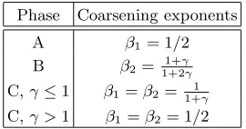
Phase Coarsening exponents

A β1= 1/2

B β2=₁₊₂1+γ_γ

C,γ≤1 β1=β2=₁₊1_γ

C,γ >1 β1=β2= 1/2

TABLE I: Coarsening exponents for asymmetric hopping

FIG. 2: Comparison of the theoretical predictions, indicated by lines, with the numerical estimates of the exponents obtained in phase A (△), B (⋄) and C (2). Errors are of the size of the symbols.

B. Comparison to simulation data

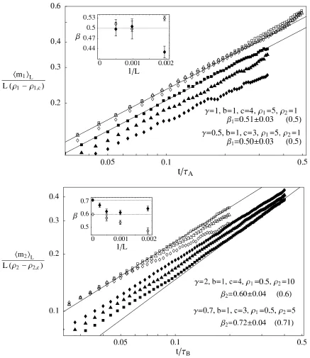
The theoretical predictions of the previous subsection are compared to Monte Carlo simulations in Figures 3 and 4.

N1= [ρ1L] resp.N2 = [ρ2L] particles of species 1 resp. 2 are initially distributed on a lattice of sizeL with uniform

probability. Cluster sites of speciesi are defined by the threshold (ρi−ρi,c)L/40. The proportionality factor has to

be chosen such that bulk fluctuations are well separated from cluster sites. Results for exponents are not sensitive to this choice for the system sizes considered, ranging fromL= 256 to 4096, since the fluctuations grow only sublinearly inL. With this threshold we measure the mean condensate sizemi(t) and other observables, such as the bulk density ρi,bulk(t), of speciesi as a function of time, scaled with the expected coarsening time scaleτ. The ensemble average

h..iL is approximated by averaging over 400 sample runs for each system size.

In the following we discuss the expected behaviour of the observables which is consistent with simulation results, up to finite size effects, discussed in the appendix. Plots of the normalized mean condensate sizehmi(t)iL/(ρi−ρi,c)Lfor

different system sizesLagainst the rescaled timet/τ, whereτ is the predicted coarsening time scale, are expected to collapse onto a single curve. Within the coarsening regime this curve should be described by the scaling laws derived in Section IV.

During nucleation, more and more particles become trapped in cluster sites, therefore the bulk densityρi,bulk(t) is a

decreasing function of time, approaching the critical densityρi,c. This is used as a criterion to identify the beginning

of the coarsening regime. The end of the coarsening regime is reached approximately whenhmi(t)iL= 0.4 (ρi−ρi,c)L,

corresponding to an average of 2.5 remaining cluster sites. For later times the data significantly deviate from the scaling law and the system saturates, as already explained in (10). Within the coarsening time regime defined above we make a linear fit to the double logarithmic data points of the normalized mean condensate size, showing an approximately linear behaviour. The measured slope gives the numerical estimate for the coarsening exponentβi. To

get sensible error estimates we slice the coarsening time window into four smaller time windows (which may overlap), and measure the exponent in each of the windows. The error βi is then taken as the standard deviation of these

measurements.

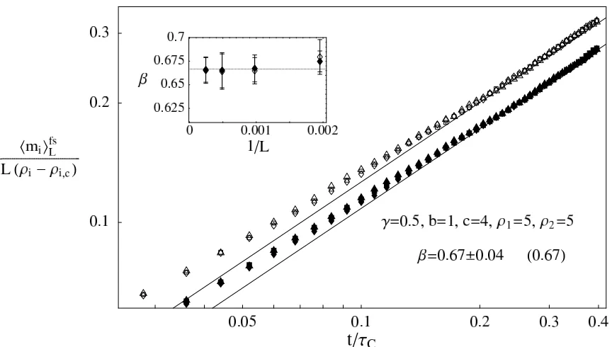
FIG. 3: Verification of the predicted scaling laws, denoted by straight lines in a double logarithmic plot of the normalized mean condensate size hmi(t)iL

L(ρ−ρc) for asymmetric hopping as a function of time. The predicted scaling exponents are given in

parentheses. The insets show the finite size scaling for the numerical estimates, where filled and unfilled symbols correspond to the data.

Top: Phase A with two sets of parameters. SymbolsL= 512(3), 1024(△), 2048(2) forγ= 1 and filled symbols forγ= 0.5.

FIG. 4: Verification of the predicted scaling laws in phase C. The plots are analogous to Figure 3, except that each one corresponds to only one value ofγand condensate sizes of both species are shown in filled and unfilled symbols.

Top: Phase C withγ= 0.5. SymbolsL= 1024(3), 2048(△), 4096(2) for species 2 and filled symbols for species 1.

Bottom: Phase C withγ= 1.5. SymbolsL= 512(3), 1024(△), 2048(2) for species 2 and filled symbols for species 1.

errors but are in good agreement with the predictions. Forγ = 1.5 we see that, as expected, the species 1 particles coarsen first, but with the same exponent as species 2 particles. In phases A and B error bars are smaller, but there are stronger finite size effects affecting the quality of the data collapse. Nevertheless the measured scaling exponents are in good agreement with the predictions.

Phase Coarsening exponents

A β1= 1/3

B β2=₂₊₃1+γ_γ

C,γ≤1 β1=β2=₂₊1_γ

C,γ >1 β1=β2= 1/3

TABLE II: Coarsening exponents for symmetric hopping.

0.05

0.1

0.2

t



Τ

0.2

0.1

X

m

\

€€€€€€€€€€€€€€€€€€€€€€€€€€€€€€€€€€€€€

L

HΡi

- Ρi,c

L

0 0.001 0.002

1



L

0.3 0.35 0.4

Β

Γ=

0.5, b

=

1, c

=

4,

Ρ1

=

5,

Ρ2

=

5

Β

=Β

=

0.38

±

0.07

H

0.4

L

FIG. 5: Verification of the predicted scaling laws for symmetric hopping in phase C withγ= 0.5. Details of the plot are given in the caption to Figure 3.

SymbolsL= 512(3), 1024(△) for species 2 and filled symbols for species 1.

C. Discussion

One can also obtain predictions for the coarsening exponents when the hopping is symmetric. In this case, there is a high probability that a particle leaving a cluster site will return to the same site. The probability that it reaches the next cluster site is inversely proportional to the distance between cluster sites [17] so it is of orderL−1_{. Therefore}

only everyO(L)-th excess particle will reach the next cluster site. Hence the coarsening time scales are increased by a factor of orderL. The assumption that excess particles move independently through the bulk remains a good one however: the time it takes particles to enter the bulk increases by a factor O(L) (compared with the driven case) since most particles return to the site they have just left; this cancels theO(L) increase in the time particles spend in the bulk due to the diffusive rather than driven motion. Then the arguments presented for the driven case with the extra factorO(L) in the coarsening time scales leads to the exponents given in Table II. We compare the prediction to preliminary simulation data in Figure 5, where we get good data collapse on the symmetric time scale. The system sizes are, however, too small for a reasonable numeric estimate of the scaling exponent, but at least one can see that the exponent is significantly smaller than for totally asymmetric hopping (cf. Figure 4 top).

For partially asymmetric hopping excess particles return to the cluster site they just left with non-zero probability, but also the probability of reaching the next cluster site in direction of the drive is of order 1, even in the limitL→ ∞. So in contrast to symmetric hopping the coarsening time scale is only corrected by a constant factor independent of

It is interesting to compare our prediction for the exponents in phase B with the results of [18] and [19] in which the authors study a single-species zero-range process where the hop rates,w1, . . . , wL, are site-dependent but independent

of the particle occupation number at the departure site. They consider symmetric [18] and asymmetric [19] dynamics, where the (quenched) hop rates are drawn independently from a distributionp(w) which can be written in the form

p(w) = [(γ−1_{+ 1)/(1−α)}γ−1₊₁

](w−α)γ−1 , (28)

wherew∈[α,1] withγ, α >0. This model undergoes a condensation transition above a critical particle density from a homogeneous phase to a phase with a condensate which resides at the site with the smallest hop rate. In both asymmetric and symmetric cases, they obtain coarsening exponents identical to those we obtain for the coarsening of the species 2 particles in phase B. One can think of the dynamics defined in (5) as a model of particles (species 2 particles) moving on an evolving disordered background (given by the species 1 particles). By the time the coarsening regime has been reached, at the cluster sites the evolving disorder is effectively quenched. Therefore it is not necessarily surprising that the two models exhibit similar coarsening behaviour for some distributionp(w). The reason the form (28) is the relevant one for the rates (5) is as follows. In the disordered model the coarsening is governed by the exchange of particles between the two slowest sites in the system. The rate at which particles are transferred between these two slowest sites is given by the difference between the two rates at these sites, ∆w. For the distribution (28), ∆w ∼L−γ/(1+γ)_{. This rate separation contributes the same factor to the coarsening time scale as that in the}

two-species model due to the dependence of the hop rate of two-species 2 particles on the background of two-species 1 particles (see equation (22)). The remaining contributions to the coarsening time scale are then determined by the symmetry of the hopping dynamics, i.e. the coarsening time scale is given by a factor of orderL for asymmetric dynamics, or a factor of orderL2 _{for symmetric dynamics, multiplied by the inverse rate separation. This leads to the same exponents as}

those obtained for phase B.

V. CONCLUSION

We have considered a two-species zero-range process which undergoes a variety of transitions to different condensate phases. The combination of two conservation laws and the coupling in the dynamics between the two species of particles leads to coarsening dynamics which are very rich compared to the single species model. In particular, we have considered a case in which the dynamics of one of the particle species (the species 2 particles) depends only on the number of particles of the other species (species 1) at the departure site, and decays to a constant value as a power law with exponent γ. While the stationary phase diagram discussed in Section II.B depends also on other system parameters, the coarsening exponents only depend (continuously) on γ and differ from phase to phase. Further, as expected, the exponents depend on the symmetry of the hopping dynamics.

AcknowledgmentsThe authors thank the Max Planck Institute for Complex Systems, Dresden, where this work was initiated, for hospitality. TH was supported by EPSRC programme grant GR/S10377/01.

APPENDIX

DISCUSSION OF FINITE SIZE EFFECTS

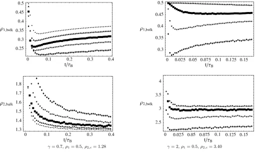
In the following we discuss qualitatively the most basic mechanisms leading to finite size effects and illustrate how they depend on the system parameters. We start with two competing effects which influence the bulk density of the condensing species, connected with the definition of cluster sites by a threshold. (i) Excess particles exchanged between cluster sites increase the bulk density in finite systems. In phase B, for example, this effect is of order

L1−γ/(1+γ)_{= L}1/(1+γ)_{, by reasoning given in Section III.B and the expansion (22). It decreases with increasing γ}

and leads to a decrease of the mean condensate size. This effect is shown forγ <1 in Figure 6 (bottom left), where

ρ2,bulk is plotted, decreasing towardsρ2,c with increasing system size L. (ii) On the other hand, bulk fluctuations

increase with γ and in finite systems they can exceed the threshold for cluster sites. This leads to an increase of the number of condensed particles, or a decrease of ρ2,bulk, which dominates over effect (i) for γ >1. This can be

seen in Figure 6 (bottom right) whereρ2,bulknow increases towardsρ2,c. Since these fluctuations are typically small

γ= 0.7,ρ1= 0.5,ρ2,c= 1.28 γ= 2,ρ1 = 0.5,ρ2,c= 3.40

FIG. 6: Finite size effects in phase B.ρ1,bulk shown on the top is smaller than its limiting valueρ1= 0.5 forL→ ∞since on

species 2 cluster sitesk1∼L1/(1+γ). With increasingγ this effect becomes weaker. ρ2,bulkshown on the bottom converges to

its limiting valueρ2,c from above (forγ <1) and from below (forγ >1) as explained in the text. Left: γ= 0.7,b= 1,c= 3,ρ1= 0.5,ρ2 = 5, critical densityρ2,c= 1.28

Symbols: L= 256(), 512(⋆), 1024(), 2048(N), 4096(•)

Right: γ= 2,b= 1,c= 4,ρ1= 0.5,ρ2= 10, critical densityρ2,c= 3.40

Symbols: L= 256(), 512(⋆), 1024(), 2048(N)

On top of these corrections, which are also present in single species models, there are mechanisms specific to two-component systems. (iv) The coarsening dynamics does not only depend on the occupation number of the condensing species, but on the relation betweenk1 and k2. As discussed above, condensates with different relations

have different lifetime. So in the limit L → ∞ ratios differing by some factor Lα _{are dynamically separated and}

only one relation dominates the coarsening. But for finite systems, ratios with shorter lifetimes also contribute to the observed behaviour. Thus data for single species systems, where this effect does not occur, are generically better than our data (cf. [2]). (v) Finally, we consider a phenomenon specific for phase B. As discussed above, on species 2 cluster sites there are of orderL1/(1+γ)_{species 1 particles due to compatibility with the bulk. Forγ <1 this is larger}

than a typical bulk fluctuation of orderL1/2_{, and reduces the bulk density of species 1 particles, whereas for γ >1}

the effect is much weaker. This can be seen in Figure 6 (top), whereρ1,bulk is plotted.

The variety of effects leads to a diverse behaviour and a quantitative prediction of the finite size corrections seems to be not feasible. However, it is straightforward to numerically fit the leading order corrections for the prefactor and the exponent of the scaling law (9), using the ansatz

mi(t)_L

(ρi−ρi,c)L =C1 1 +C2/L δ1t

τ

βi+C3/Lδ2

. (29)

Consider for instance the data in phase C withγ= 0.5 given in Figure 4 (top). The finite size corrections in the inset suggestδ2 = 1 and the best fit values for the other parameters areδ1= 0.69, C1 = 0.51, C2 = 2.3, C3 =−21 for

species 1 andδ1= 0.60, C1= 0.59, C2= 2.1, C3=−13 for species 2. In Figure 7 we plot the corrected data

mi(t) f s L

(ρi−ρi,c)L =

mi(t)_L

(ρi−ρi,c)L

t

τ

−C3/Lδ2

C1+C2/Lδ1

−1

FIG. 7: Finite size corrected data for phase C withγ= 0.5 as given in (30).

and the data collapse improves drastically.

[1] M. R. Evans, Braz. J. Phys.30(2000) 42

[2] S. Großkinsky, G. M. Sch¨utz and H. Spohn, J. Stat. Phys.113(2003) 389 [3] C. Godr`eche, J. Phys. A36(2003) 6313

[4] Y. Kafri, E. Levine, D. Mukamel, G. M. Sch¨utz and J. T¨or¨ok, Phys. Rev. Lett. 89, 035702 (2002) [5] M. R. Evans, E. Levine, P. K. Mohanty and D. Mukamel, Eur. Phys. J. B41(2004) 223-230 [6] J. D. Noh, G. M. Shim and H. Lee, cond-mat/0409120

[7] A. G. Angel, M. R. Evans and D. Mukamel, J. Stat. Mech.: Theor. Exp. (2004) P04001 [8] O. Pulkkinen, J. Merikoski, cond-mat/0411630

[9] M. R. Evans and T. Hanney, J. Phys. A36(2003) L441 [10] T. Hanney and M. R. Evans, Phys. Rev. E69(2004) 016107 [11] G. M. Sch¨utz, J. Phys. A36(2003) R339

[12] R. Mikkelsen, D. van der Meer, K. van der Weele and D. Lohse, Phys. Rev. Lett.89(2002) 214301 [13] S. N. Dorogovtsev, J. F. F. Mendes and A.N. Samukhin, Nucl. Phys. B666(2003) 396

[14] S. Großkinsky and H. Spohn, Bull. Braz. Math. Soc34(2003) 1 [15] S. Großkinsky, in preparation

[16] A. J. Bray, Adv. Phys.43(1994) 357 and51(2002) 481 (reprint)

[17] G. H. Weiss,Aspects and Applications of the Random Walk, North-Holland, Amsterdam (1994) [18] M. Barma and K. Jain., Pramana - J. Phys.58(2002) 409