The radial plot in meta analysis : approximations and applications

University of Warwick institutional repository: http://go.warwick.ac.uk/wrap

This paper is made available online in accordance with publisher policies. Please scroll down to view the document itself. Please refer to the repository record for this item and our policy information available from the repository home page for further information.

To see the final version of this paper please visit the publisher’s website. Access to the published version may require a subscription.

Author(s): JB Copas and C Lozada-Can

Article Title: The Radial Plot in Meta Analysis: Approximations and Applications

Year of publication: 2009 Link to published article:

The Radial Plot in Meta Analysis: Approximations and

Applications

John Copas

University of Warwick, UK

and Claudia Lozada-Can

´

Ecole Polytechnique F´ed´erale de Lausanne, Switzerland

Summary

Fixed effects meta analysis can be thought of as least squares analysis of the radial plot, the plot of standardized treatment effect against precision (reciprocal of the standard deviation) for the studies in a systematic review. For example, the least squares slope through the origin estimates the treatment effect, and a widely used test for publication bias is equivalent to testing the significance of the regression intercept. However, the usual theory assumes that the within-study variances are known, whereas in practice they are estimated. This leads to extra variability in the points of the radial plot which can lead to a marked distortion in inferences derived from these regression calculations. This is illustrated by a clinical trials example from the Cochrane Database. We derive approximations to the sampling properties of the radial plot and suggest bias corrections to some of the commonly used methods of meta analysis. A simulation study suggests that these bias corrections are effective in controlling significance levels of tests and coverage of confidence intervals.

Key words_{: Meta analysis; Radial plot; Bias corrections; Publication bias; Egger test.}

1

Introduction and example

The standard fixed effects model in meta analysis is that we have k separate studies, each reporting an estimate ˆθ of a common parameter θ. Each estimate (typically a treatment effect) is assumed to be independent and normally distributed

ˆ

θ _∼N(θ,σ

2

n ), (1)

wherenis the sample size andσ2_{an underlying variance parameter. Note thatθis common}

(the fixed effects assumption) but n and σ2 _{will usually vary across the studies. Given}

(ˆθi, σi2, ni) for the k studies, the maximum likelihood estimate of θ, and its variance, are

˜

θ= P

niσi−2θˆi P

niσ−i 2

, σ2_θ˜ =

1 P

niσi−2

. (2)

Confidence intervals and tests for θ are based on the fact that

Z1 = (

X

niσ−i 2)

1

2(˜θ−θ) (3)

has a standard normal distribution.

A good way of looking at (ˆθi, σ2i, ni) in a meta analysis is to plot the data as a Radial

Plot (Galbraith, 1988). This plots the standardized treatment effect against the precision (one over the standard error) of each study, or y againstx where

y= θˆ

√_n

σ and x=

√_n

σ . (4)

In terms of the radial plot, (1) is the linear regression model

y =α+θx+ǫ, (5)

where α= 0 and ǫ is a standard normal residual. Thus, if the model is correct, the plot of standardized effects against study precision should be a straight line radiating out from the origin, with slope equal to the true value of θ and known residual variance equal to one. Further, ˜θ is just the slope of the least squares line through the origin, so (2) and (3) are the familiar regression calculations

˜

θ = sxy

sxx

, σ_θ2˜=

1

ksxx

, Z1 = (ksxx)

1

2(˜θ−θ).

In this and throughout the paper we use the generic notation, for any k pairs of numbers (ai, bi),

sab = 1

k

X

i

aibi , cab = 1

k

X

i

(ai−¯a)(bi −¯b) .

See Sutton et al. (2000) for a good general introduction to meta analysis and radial plots. For reasons that will become clear later, we have used a slightly different notation from that usually used in meta analysis. By defining the variance of ˆθ to be σ2_{/n rather than}

As the motivating example for this paper, Table 1 reports the results of 11 clinical trials into the effectiveness of iron supplementation in pregnancy. This example comes from the Cochrane database (Pena-Rosas and Viteri, 2006; Schwarzer et al., 2007). The entries in Table 1 are observed frequencies, for example in the first trial the number of adverse events (low haemoglobin level in late pregnancy) was 0 out of 30 patients on treatment (f1 out of

m1) and 14 out of 25 patients on control (f2 out ofm2). The data clearly suggest that iron

supplementation has a very strong beneficial effect. If θ is the underlying log odds ratio measuring the treatment effect, then for each study the usual estimate of θ is

ˆ

θ= log

(f1+ 0.5)(m2−f2+ 0.5)

(m1−f1+ 0.5)(f2+ 0.5)

, (6)

with variance σ2 _{taken to be}

ˆ

σ2 _=n

1

f1+ 0.5

+ 1

m1 −f1+ 0.5

+ 1

f2+ 0.5

+ 1

m2−f2+ 0.5

, (7)

wheren is the total study sample sizen =m1+m2. In these calculations we have followed

the standard convention of adding 0.5 onto each frequency to improve bias and avoid prob-lems with sparse data. Substituting these values into (2) gives the meta analysis estimate of θ to be ˜θ =₋1.906 with standard errorσ_θ˜= 0.191.

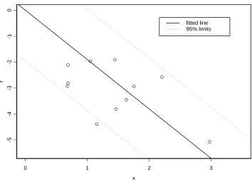
To visualize the model, Figure 1 shows the radial plot for these data. The fit of the fixed effects model is confirmed by the three parallel straight lines drawn on this graph,

y = ₋1.906x (solid line) and y = ₋1.906x_±1.96 (dotted lines). Ten out of the eleven points lie between the outer lines, consistent with the point-wise 95% coverage probabilities implied by (5).

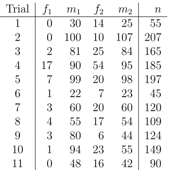
Trial f1 m1 f2 m2 n

1 0 30 14 25 55

2 0 100 10 107 207

3 2 81 25 84 165

4 17 90 54 95 185

5 7 99 20 98 197

6 1 22 7 23 45

7 3 60 20 60 120

8 4 55 17 54 109

9 3 80 6 44 124

10 1 94 23 55 149

11 0 48 16 42 90

Table 1. Iron supplementation meta analysis.

Although the radial plot suggests a reasonable fit of the model, we know that the model cannot be exactly correct because we have ignored the fact that (7) is merely an estimate and not the true variance of each study. As mentioned, the validity of the usual analysis depends on the distribution ofZ1 being standard normal. We can check this by estimating

estimate ˜θ =₋1.906 as if it was the true value of θ, and estimate the probabilities (p1, p2)

for the two arms of each trial so that they have ₋1.906 as their common log-odds ratio (details of how to do this will be discussed later in Section 3). We then simulate sets of 2_×2 tables by generating random observations from the binomial distributionsf1 ∼bin(m1, p1)

andf2 ∼bin(m2, p2). Each set of tables gives a new estimate ˜θand hence a value ofZ1 with

θ =₋1.906. The dashed line in Figure 2 shows the kernel density estimate of Z1 based on

10,000 simulations. This is clearly different from the nominal standard normal distribution shown as the solid line. The distortion is a substantial shift to the right. The fact that the variance stays about the same suggests that for valid confidence intervals we should adjust the value Z1 with a bias correction before assuming it is standard normal. The

vertical dotted line in Figure 2 indicates the value of E(Z1) calculated from the asymptotic

formula to be developed later in Sections 2 and 3. We see that subtracting this bias from

Z1 successfully restores the distribution to N(0,1), at least approximately. The object of

our paper is to show how we can improve meta analysis calculations by developing bias corrections of this kind. We will return to this example again in Section 3.

Other standard methods in meta analysis can also be reduced to regression-like calcu-lations on the radial plot. The residual sum of squares from the least squares line through the origin,

Q=ksyy−

ks2

xy

sxx

=X

i

ni

σ2

i

(ˆθi−θ˜)2 , (8)

is just the usual “Q-statistic” for testing heterogeneity between the studies. Under the fixed effects model (1), Q is chi-squared on (k₋1) degrees of freedom. A large value ofQ

indicates that there are systematic differences between the studies — the usual approach is then to use Qto estimate the random effects variance in a random effects model (Suttonet al., 2000, section 5.2). The model assertion that the intercept of the radial plot is zero can also be tested, by fitting an unconstrained least squares line to the radial plot and testing its intercept to give the test statistic

Z2 =

kcxx

sxx

1₂

(¯y₋θ˘x¯) , θ˘= cxy

cxx

. (9)

Under the model, Z2 is standard normal. Testing Z2 is equivalent to the “Egger test”,

widely used in meta analysis to test for publication bias or a “small study effect” (Egger

et al., 1997). Finally, testing significance of the slope ˘θ of the unconstrained least squares line provides another way of testing the treatment effect (that θ₆= 0). Under the model (1) this is less powerful than the test based on Z1, but Copas and Malley (2008) show that it

is much more robust to publication bias. This gives the robust test statistic

Z3 = (kcxx)

1

2θ ,˘ (10)

again standard normal under the model.

The example has already highlighted the main cause of bias, that in practice we have to use estimates ˆσ2 _{instead of the true study-specific variances σ}2 _{when plotting radial plots}

and calculating these various quantities. So from now on we replace (4) by

y= θˆ √

n

ˆ

σ and x=

√

n

ˆ

Replacing σ by ˆσ inxand y upsets the assumptions necessary for the linear regression (5). The stochastic error inxmay lead to bias in the parameter estimates, and the variability in ˆ

σ may also induce a within-study correlation between xand y. Both effects mean that the distributions stated for Z1, Q, Z2 and Z3 are no longer valid. Although this problem has

been widely acknowledged, little work seems to have been done to explore its consequences. An exception is the Egger test, where several recent simulation studies (Macaskill et al., 2001; Schwarzer et al., 2002; Peterset al., 2006; Harbordet al., 2006) have shown that the true significance level can be substantially inflated, meaning that the test rejects the null hypothesis more often than it should.

In Section 2 of this paper we study the distribution ofxandyin (11) and give asymptotic approximations to some of the sampling properties of the radial plot, asymptotic in the sense that the study-specific sample sizes are large. This leads in Section 3 to bias corrections to the various statistics listed above, and hence to improved control of significance levels of tests and coverage of confidence intervals. We also return to the example in Section 3, and then report the results of a simulation study in Section 4. Brief comments and conclusions are listed in Section 5. The Appendix outlines the derivation of some of the formulae used in Sections 2 and 3.

2

Asymptotic theory of radial plots

Since there arek different sample sizes ni in a meta analysis, we first need to be clear what we mean by “asymptotic”. The accuracy of the approximations developed below are stated in terms of the overall sample sizeN =Pk

1ni, assuming that the proportional sample sizes

ni/N are fixed. Our numerical results suggest that in practice these approximations will be useful provided that the sample sizes in the majority of studies are not too small.

Properties of the radial plot coordinates x and y in (11) depend on the statistical properties of ˆθ and ˆσ2_{, and hence on the type and design of the studies being combined in}

the meta analysis. We show in the Appendix that there are three important quantities for each study:

a= n

Nσ2

1₂

, b= E (

(nN)12(ˆθ−θ)

ˆ

σ

)

, d= E (

n(ˆθ₋θ)(ˆσ₋σ)

σσˆ2

)

. (12)

The quantity a is defined directly in terms ofn and σ2_{. Two special cases of interest for b}

and d are:

Special case 1: normal data. If, in each study, ˆθ is the sample mean of a random sample of size n fromN(θ, σ2) and ˆσ2 is the sample variance, then ˆθ and ˆσ2 are independent and so b=d= 0.

study gives an estimated log-odds ratio ˆθ in (6) with estimated variance ˆσ2 _{in (7).}

The corresponding study parameters are

θ = logp1(1−p2) (1₋p1)p2

and σ2 =γ1+γ2 , (13)

where

γj =

n mjpj(1−pj)

; j = 1,2. (14)

In this case, ˆθ and ˆσ2 _{can be substantially correlated, and we show in Appendix A2}

that for large n,

b =₋d

a , d= γ2

2(1−2p2)−γ12(1−2p1)

2(γ1+γ2)2

. (15)

With estimated within-study variances, ˜θis no longer an unbiased estimate ofθ, but has a bias of orderO(N−1). This means that ifN is large the bias in ˜θ is small compared to its

standard error which is of orderO(N−1₂). Similarly, it turns out that E(Q) =k−1+O(N−1).

However, for tests and confidence intervals we need the quantities Z1, Z2, Z3, and each of

these has a bias of order O(N−1₂). The size of the bias depends on the values of (a, b, d) in

each study. Explicitly, we show in Appendix A3 that

E(Zj) = AjN−

1

2 +O(N−1) ; j = 1,2,3, (16)

where

A1 =

k saa

1₂

sab−d¯+

sa2_d ksaa

, (17)

A2 =

k caas3aa

1₂

×

saa(caa¯b−cab¯a)− 1

k

cad(2¯a2₋saa)₋(k₋2)saa¯ad¯₋ ¯ac(a−a¯)2d

caa

(2saa −a¯2)

, (18)

and

A3 =

k caa

1₂

cab−

1₋ 2

k

¯

d+c(a−¯a)2d

kcaa

. (19)

Note that the study-specific values (a, b, d) enter into the bias terms through the averages and average squares and products ¯a, saa,sab etc.

3

Bias corrections

We show in Appendix A3 that

Var(Zj) = 1 +O(N−1) ; j = 1,2,3 . (20)

compared an estimate of the density of Z1 in the medical example with the density of the

standard normal.

If we ignore terms of order O(N−1) but allow for the bias in Z

1 of order O(N−

1 2), a

normal approximation forZ1 gives the adjusted confidence interval for θ with limits

˜

θ₋(ksxx)−1₂{Aˆ

1N−

1

2 ±z_α} , (21)

where ˆA1 is an estimate ofA1 in (17) andzαis the standard normal percentage point needed to achieve the desired coverage (1₋α). The conventional confidence interval is just (21) with the bias term omitted. The analogous two-sided P-value for treatment effect is

P = 2Φ_{−|(ksxx)12θ˜−Aˆ₁N−1₂|} , (22)

where Φ is the standard normal cumulative distribution function. Similarly, the adjusted two-sided P-values for tests based onZ2 and Z3 are

2Φ_{−|Z2−Aˆ2N−

1

2|} and 2Φ{−|Z₃ −Aˆ₃N−1₂|} . (23)

To implement these adjustments we have to estimate A1, A2 and A3 using (17), (18) and

(19). Again these depend on the nature of the studies being combined.

Special case 1: normal data. Here b =d= 0 for all studies, so all three quantities Aj are zero. No bias corrections are needed in this case. Of course the procedures are still biased, but the biases are of a lower order of magnitude.

Special case 2: 2_×2 tables. From (12) and (13),

a=

r _n

N(γ1+γ2)

. (24)

This, together with (15), shows that (a, b, d) can all be written as functions of the values of (γ1, γ2) and hence of (p1, p2) in the k studies. To estimate (p1, p2) we should

exploit the fixed effects assumption, that the pairs (p1, p2) are related through a

common log-odds ratio. The constrained maximum likelihood estimates ofp1 and p2

given that

Θ(p1, p2) = log

p1(1−p2)

(1₋p1)p2

= ˜θ

are

p1(λ) =

f1+λ+ 0.5

m1 + 1

and p2(λ) =

f2−λ+ 0.5

m2+ 1

, (25)

where λ is a Lagrange multiplier given by solving the quadratic equation

Θ_{p1(λ), p2(λ)}= ˜θ . (26)

For consistency with the earlier definitions of x and y, we have again added one half onto all of the observed frequencies in these calculations. By examining the function Θ(p1, p2) it is easy to check that (26) has two real solutions and that it is the larger

solution for λ which gives values of p1 and p2 in [0,1]. Thus, to estimate (a, b, d)

for each study, we find λ from (26), (p1, p2) from (25), (γ1, γ2) from (14) and hence

Since the special case of 2_×2 tables is the most commonly occurring example in medical applications, we now set out these calculation more explicitly. We havek studies each with data f1 ∼bin(m1, p1) and f2 ∼bin(m2, p2). The steps are

• First calculate the study-specific estimates (ˆθ,ˆσ2_{) in (6) and (7), and hence the usual}

radial plot co-ordinates (x, y) in (11) and the radial plot regression statistics of inter-est.

• Letη = exp(˜θ). If η₆= 1, calculate the Lagrange multipliers

λ = _{2(1₋η)_}−1[− {f

1+m2−f2+ 1 +η(f2+m1−f1+ 1)}

+

{f1+f2 −m2+η(m1−f1−f2)}2+ 4η(m1+ 1)(m2+ 1)

1 2

i

,

and hence each study’s estimate of (p1, p2) in (25). Ifη= 1 (no treatment effect) then

we simply take ˆp1 = ˆp2 = (f1 +f2 + 1)/(m1 +m2 + 2). We can now calculate the

estimates (ˆγ1,γˆ2) from (14) and hence the following three quantities for each study:

ˆ

a =

r _n

N(ˆγ1+ ˆγ2)

, dˆ= γˆ

2

2(1−2ˆp2)−γˆ12(1−2ˆp1)

2(ˆγ1+ ˆγ2)2

, ˆb =₋dˆ ˆ

a .

• Calculate the average values across thek studies of the quantities (ˆa,ˆb,d,ˆaˆ2_,(ˆa−¯ˆ_a)2₎

and the empirical mean squares and covariances needed to find ˆA1, ˆA2 or ˆA3 from

(17), (18) or (19). These give the bias corrections for the tests or confidence intervals specified in (21), (22) and (23).

To illustrate these calculations we return to the medical example mentioned in

Section 1, with data set out in Table 1. First we fit the fixed effects model to the observed 2_×2 tables by estimating (p1, p2) as explained above, and hence calculate estimates of

(a, b, d) for each study, and hence the bias corrections for Z1 and Z2. The null hypothesis

being tested by Z3 is H0 : θ = 0, and so to estimate the bias correction for Z3 we fit the

null model instead (η= 1 in the above notation). The results are as follows:

Confidence interval for θ. The conventional estimate of the log-odds ratio is ˜θ=₋1.906 with standard error 0.191. This gives the usual 95% confidence interval

−1.906_±1.96_×0.191 = (₋2.280,₋1.532).

The bias estimate ˆA1N−

1

2 is +0.879 giving the corrected confidence interval

−1.906₋0.191_×(0.879_±1.96) = (₋2.447,₋1.700).

Intercept test for publication bias. The value of (9) is Z2 = −2.844 giving the

con-ventional P-value as P = 0.004, highly significant evidence for publication bias. The bias estimate ˆA2N−

1

2 is−0.927, and so the bias adjusted P-value in (23) isP = 0.055,

suggest-ing that the real evidence is substantially weaker than the naive analysis suggests. This agrees with the analysis of this example in Schwarzer et al. (2007), who also conclude that the evidence for publication bias provided by the conventional intercept test is much exaggerated.

Unconstrained test of treatment effect. The evidence for a non-zero treatment effect is extremely strong when judged by the confidence intervals discussed above, with or without the bias correction on Z1. However the intercept test raises doubts about publication bias,

even with the bias correction onZ2 the P-value only just exceeds 5%. It is well known that

if there is a selection effect in meta analysis then to ignore it can be extremely misleading. Thus, following Copas and Malley (2008), it might be thought safer in this case to allow for the possibility of a selection effect, and use the robust test based on Z3. The value of

(10) comes to Z3 = −1.698, giving a nominal P-value of P = 0.090: the evidence for the

treatment effect is now much weaker. The bias correction ˆA3N−

1

2 is−0.0818, adjusting the

P-value in (23) to P = 0.106. In this case the bias correction to Z3 is unimportant, but

allowing for publication bias has been catastrophic as far as the conclusion of this particular meta analysis is concerned.

4

Simulation study

In this section we give a very brief summary of some simulation results exploring the accu-racy of our approximations. We only report results here for the special case of 2_×2 tables, and for perhaps the two most common tasks in meta analysis, confidence intervals and P-values for θ, and the intercept (Egger) test for publication bias. Clearly it is impossible to cover all possibilities: we illustrate our results by looking at the distributions of Z1 and

Z2 in a few representative cases, and suggest some qualitative conclusions.

For Figures 3 and 4, and Table 2, we have taken k= 50, generated random sample sizes

m1 andm2 uniformly between 150 and 300, and definedpE, the average ofp1 andp2 on the

logit scale, to be 0.3. For any true value ofθwe can then generate random 2_×2 tables, and for each set of tables calculate the statistics of interest and estimate their bias corrections as set out in Section 3. The simulations are repeated 100,000 times.

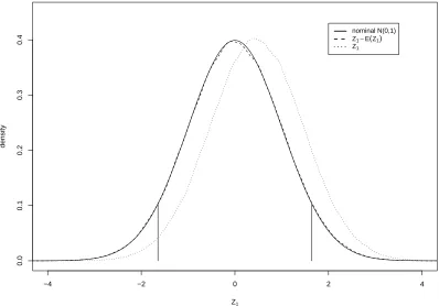
Figure 3 looks at Z1 with θ = log(0.2) and shows kernel density estimates of the

distri-bution ofZ1, and of the bias corrected versionZ1−Aˆ1N−

1

2. The distribution ofZ₁−Aˆ₁N−1₂

is virtually indistinguishable from the standard normal, but the distribution of Z1 is

no-ticeably shifted to the right, in the same direction as the bias noted earlier for the example in Figure 2. In Figure 3, the estimates of E(Z1) have been very effective at removing the

bias.

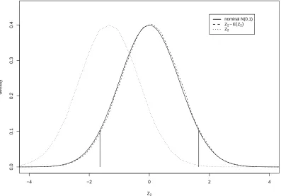
Figure 4 takes θ = log(0.5) and shows kernel density estimates of the distribution ofZ2

and of the bias corrected version Z2−Aˆ2N−

1

2. Here there is an even larger shift, this time

to the left, but again the distribution ofZ2−Aˆ2N−

1

standard normal.

The short vertical lines on these figures indicate the 5th and 95th percentiles of the stan-dard normal distribution. Thus the areas to each side of these lines indicate the actual sig-nificance levels of tests based onZ1 andZ2, or equivalently the actual coverage of confidence

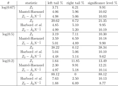
intervals based onZ1. The results are summarized in Table 2 forθ = log(0.67),log(0.5) and

log(0.2). For the cases shown, the distortion in significance levels is particulary severe for the intercept testZ2, these figures being in line with the findings of Macaskillet al. (2001),

Schwarzer et al. (2002), Peters et al. (2006) and Harbord et al. (2006). In all rows of the table, bias is indicated by an imbalance between the left and right tail error rates.

Radial plot methods apply to meta analysis problems rather generally, but for the specific case of 2_×2 tables other methods are also available, notably the Mantel-Haenszel estimate (Mantel and Haenszel, 1959; Mantel, 1963). This estimate works directly on odds ratios without the logarithmic transformation, and so is not a function of the radial plot as defined here. For completeness we have included in Table 2 the analogous results for the Mantel-Haenszel method, using the analogue of Z1 for the logarithm of the

Mantel-Haenszel estimate and the variance estimate of Robins et al. (1986). For the intercept test (Egger test) based on Z2, we can also compare our results with the recently proposed test

of Harbord et al. (2006). Again their test is specific to the 2_×2 case and is not a function of the radial plot. In Table 2 we include error rates for the Harbord et al. test statistic in place of Z2.

θ statistic left tail % right tail % significance level %

log(0.67) Z1 3.71 6.21 9.91

Mantel-Haenszel 4.06 5.96 10.02

Z1−Aˆ1N−

1

2 4.98 5.06 10.03

Z2 20.62 0.72 21.35

Harbordet al. 4.85 5.10 9.95

Z2−Aˆ2N−

1

2 4.99 5.20 10.19

log(0.5) Z1 3.19 7.11 10.30

Mantel-Haenszel 3.59 6.59 10.18

Z1−Aˆ1N−

1

2 5.01 4.89 9.90

Z2 38.22 0.12 38.34

Harbordet al. 5.04 5.06 10.10

Z2−Aˆ2N−

1

2 4.48 5.14 9.62

log(0.2) Z1 1.64 11.85 13.49

Mantel-Haenszel 2.30 9.91 12.21

Z1−Aˆ1N−

1

2 4.97 5.18 10.14

Z2 88.12 0 88.12

Harbordet al. 7.63 2.50 10.13

Z2−Aˆ2N−

1

2 1.88 6.89 8.77

Table 2. Error rates for nominal 10% (two-sided) and 5% (one-sided) confidence intervals and tests.

some tentative conclusions about how the biases of Z1,Z2 and Z3 depend on the particular

characteristics of the meta analysis. We find:

• bias tends to increase with k, the number of studies

• bias tends to increase with _|θ_|(the stronger the treatment effect)

• bias tends to increase as the average response probability pE becomes more extreme (nearer 0 or 1)

• bias tends to decrease as the sample sizes m1 and m2 increase

• bias tends to increase as the trials become more unbalanced (m1 different fromm2)

• bias is relatively insensitive to variations in p1 and p2 between trials (trials have the

same value of θ but different values ofpE)

• on the whole, bias is more marked for the intercept test Z2 than for the tests or

confidence intervals based onZ1 and Z3

• the accuracy of the bias estimates deteriorates as the data become more sparse (m1

and p1, or m2 and p2, both small). These are cases, however, where bias can be

particularly severe, but the bias corrections can still be worthwhile in the sense of being less misleading than the conventional statistics (this is clearly shown in the last part of Table 2 where theZ2 test is grossly misleading: at this setting there are likely

to be several zeros in the data).

Table 2 suggests that the Mantel-Haenszel method suffers a bias rather similar to that of Z1, suggesting that a bias correction to this estimate would also be useful. Table 2 also

shows (at least for the cases considered) that the test of Harbord et al. (2006) is effective in reducing the bias of the Egger test. At more extreme values of θ, seen in the last part of Table 2, there is a tendency for Harbord et al. to under-correct, and for Z2−Aˆ2N−

1 2 to

over-correct, for this bias, although the (two-tail) significance levels are quite similar (and dramatically better than the significance level of Z2).

5

Conclusions and comments

1. The variance-weighted estimate ˜θin (2), widely used in meta analysis, can be thought of as the slope of a linear regression through the origin of the radial plot (plot of standardized treatment effects against one over their standard errors). Tests and confidence intervals for

setting for investigating and correcting for these biases. At least for the cases discussed above, these biases can be quite substantial. Provided _|θ_|, the size of the treatment effect, is not too large, the bias corrections proposed here seem effective and will be useful in practice.

2. The bias corrections in Section 3 depend on the quantities (a, b, d) for each study, and hence on the statistical properties of the studies being combined. We have evaluated these explicitly for the case of normally distributed observations and for the case of 2_×2 tables. However, meta analysis is used much more widely, for example the case of estimated log hazard ratios in survival studies would also be of interest. Insight into the statistical properties of (ˆθ,ˆσ2_{) is needed for estimating (a, b, d) and so is a pre-requisite for estimating}

bias corrections for the resulting meta analysis.

3. We have referred toZ2 as the intercept test rather than the Egger test, to make the

technical distinction thatZ2 uses the fact that the residual variance of the radial plot under

the fixed effects model is known to be one, whereas the Egger test often uses the estimated residual mean square as in standard regression analysis. Although less efficient than Z2

under the fixed effects model, using the observed residual mean square has the advantage of being more robust to heterogeneity between the studies.

4. For completeness we have also included the Mantel-Haenszel and Harbord et al.

methods in Table 2 since these are also available in the special case of 2_×2 tables. There is a large literature on the Mantel-Haenszel estimate and how it compares with the variance-weighted approach, see Sutton et al. (2000, section 4.3.5) for a summary. The consensus in most of this literature is that Mantel-Haenszel is better if there is a large number of small studies, but ˜θ is better for a small number of large studies. It is unclear how these conclusions would be affected if bias corrections were introduced. The test proposed by Harbord et al. (2006) is just one of several other recently proposed improvements to the Egger test (Macaskill et al., 2001; Peterset al., 2006; R¨ucker et al., 2008; Schwarzer et al., 2007). These may be effective (and simpler) alternatives to using the bias correction for

Z2, but their comparative properties have yet to be fully evaluated.

5. We have assumed the fixed effects model throughout. The usual practice is to test this assumption by calculating Qin (8) and if this is significant as χ2 _{on (k−1) degrees of}

freedom to estimate a between-studies varianceτ2 _{and use the random effects model instead}

(Suttonet al., 2000, section 5.2). Essentially, this is equivalent to redefining the radial plot coordinates by replacing σ2_{/n by τ}2 _+σ2_{/n. The conventional calculations of ˜θ and Z}

1

take exactly the same form, but the bias E(Z1) will change. Simulations suggest that when

τ2 _{is small the size of this bias is quite similar, but we have no theory to back this up.}

To fully rework the theory of Section 2 for the random effects model would be much more challenging, as estimates of τ2 depend on all the data and not just on the individual points in the radial plot. The literature shows that allowing for the uncertainty in ˆτ2_{, especially}

with the truncation usually used to avoid negative variance estimates, is difficult enough without adding the complication of uncertainty in the ˆσ2

6. The bias formulae for the case of 2_×2 tables simplify for two special (but important) cases, when the two arms of each trial are balanced (m1 = m2 in all trials), and for the

null hypothesis H0 (p1 = p2 in all trials). If both of these hold (balanced trials with no

treatment effect), the biases are all zero since d= 0 in (15). In particular, both Z1 and Z3

provide approximately unbiased tests for the significance of the overall treatment effect in the important case of balanced clinical trials, when no bias corrections are needed.

Acknowledgement

We are grateful to referees for their helpful comments. One of us (CL-C) was supported by CONACYT (Mexico) grant no. 160859.

References

Copas, J. B. and Malley, P. F. (2008). A robust P-value for treatment effect in meta analysis with publication bias. Statist. in Med., 27, 4267-4278.

Egger, M., Smith, G. D., Schneider, M. and Minder, C. (1997). Bias in meta analysis detected by a simple graphical test. Brit. Med. J., 315, 629-634.

Galbraith, R. F. (1988). A note on graphical representation of estimated odds ratios from several clinical trials. Statist. in Med., 7, 889-894.

Harbord, R. M., Egger, M. and Sterne, J. A. C. (2006). A modified test for small study effects in meta analysis of controlled trials with binary endpoints. Statist. in Med.,

25, 3443-3457.

Macaskill, P., Walter, S. D. and Irwig, L. (2001). A comparison of methods to detect publication bias in meta analysis. Statist. in Med., 20, 641-654.

Mantel, N. (1963). Chi-squared tests with one degree of freedom: extension of the Mantel-Haenszel procedure. J. Am. Statist. Assoc., 58, 690-700.

Mantel, N. and Haenszel, W. (1959). Statistical aspects of the analysis of data from retrospective studies of disease. J. Nat. Cancer Inst.,22, 719-748.

Pena-Rosas, J, P. and Viteri, F. E. (2006). Effects of routine oral iron supplementation with or without folic acid for women in pregnancy. Cochrane Database of Systematic Reviews, 2006, Issue 3, Art No.: CD004736. DOI: 10.1002/14651858.CD004736.pub2.

Peters, J. L., Sutton, A. J., Jones, D. R., Abrams, K. R. and Rushton, L. (2006). Com-parison of two methods to detect publication bias in meta analysis. J. Am. Med. Assoc., 295, 676-680.

Robins, J., Breslow, N and Greenland, S. (1986). Estimators of the Mantel-Haenszel variance consistent in both sparse and large-stratum limiting models. Biometrics,

R¨ucker, G., Carpenter, J. R. and Schwarzer, G. (2008). Arcsin tests for publication bias.

Statist. in Med., 27, 746-763.

Schwarzer, G., Antes, G. and Schumacher, M. (2002). Inflation in Type I error rate in two statistical tests for the detection of publication bias in meta analysis with binary outcomes. Statist. in Med., 21, 2465-2477.

Schwarzer, G., Antes, G. and Schumacher, M. (2007). A test for publication bias in meta-analysis with sparse data. Statist. in Med.,26, 721-733 .

Sutton, A. J., Abrams, K. R., Jones, D. R., Sheldon, T. A. and Song, F. (2000). Methods for meta-analysis in medical research. Chichester: Wiley.

Appendix

Here is an outline of the derivation of some of the formulae quoted in Section 2 and 3:

A1 : Approximations for a single study

Model (1) states that ˆθis asymptoticallyN(θ, σ2_{/n); first we extend this to suppose that}

(ˆθ,σˆ2_{) is asymptotically jointly normal with mean (θ, σ}2_{). We assume that the biases in both}

estimates are of order O(n−1), that Var(ˆθ) =σ2/n+O(n−2), and that Var(ˆσ2) =O(n−1).

These are standard properties of maximum likelihood estimates; in practice they will hold for any ‘sensible’ estimates of θ and σ2_.

Now define

u=x₋

√

n σ =

√

n

1 ˆ

σ −

1

σ

, v=y₋θ

√

n σ =

√

n θˆ

ˆ

σ − θ σ

!

, w =v₋θu= (ˆθ−θ) √

n

ˆ

σ .

(27) Then

b =N12E(w) and d=−E(uw) ,

both of which are of orderO(1) asN _{→ ∞}. Also as a consequence of the above assumptions we have

E(u) =O(n−1₂) , Var(w) = 1 +O(n−1) and Cov(w, uw) = O(n−₂1). (28)

A2 : Special case 2: 2_×2 table

First consider the case of a single binomial distribution, with observed frequency

f _∼ bin(m, p), say. Letz be the asymptotic (largem) standard normal deviate correspond-ing to f, that is

z = f_p−mp

m/γ and γ =

1

Then after some tedious but straightforward algebra we find

log f +

1 2

m₋f +1₂ = log

p

1₋p+γ 1

2zm−1₂ +1

2γ(1−2p)(1−z

2_)m−1 +Op(m−3/2), (29)

m+ 1 (f +1

2)(m−f + 1 2)

=γm−1

−γ3/2(1₋2p)zm−3/2 _+Op(m−2_{). (30)}

Now extend this to two binomial distributions f1 ∼ bin(m1, p1) and f2 ∼ bin(m2, p2),

with n = m1 +m2 and (ˆθ,σˆ2) defined in (6) and (7). We use (29) and (30) to expand ˆθ

and ˆσ2 _{in powers of n}−1₂ and in terms of two independent standard normal deviates z

1 and

z2. With (14) this leads to

u= 1

2(γ1+γ2)

−3/2{γ3/2

1 (1−2p1)z1+γ23/2(1−2p2)z2}+Op(n−

1 2),

and

w = (γ1+γ2)−

1 2(γ

1 2

1z1 −γ

1 2

2z2) +

1 2n

−1₂

h 2u(γ12

1z1−γ

1 2

2z2)

+ (γ1+γ2)−

1

2{γ₁(1−2p₁)(1−z2

1)−γ2(1−2p2)(1−z22)}

i

+Op(n−1).

which in turn lead to (15).

A3 : Approximations for radial plot statistics

From (27) and (12) we get

x= √

n

ˆ

σ =aN 1

2 +u and y=

ˆ

θ√n

ˆ

σ =aθN 1 2 +v .

Hence

sxx = Nsaa+ 2N

1

2s_au+s_uu , sxy = θNsaa +N

1

2(s_av+θsau) +s_uv

= θsxx+N

1

2s_aw+s_uw .

These lead to

˜

θ = θ+saw

saa

N−1₂ +Op(N−1) (31)

Z1 =

k saa

1₂

saw+

suw −

sawsau

saa

N−1₂

+Op(N−1) (32)

Q = k

sww−

s2

wa

saa − 2swa

s2

aa

(saasuw −sausaw)N−

1 2

+Op(N−1). (33)

The expectations of the random quantities appearing in (31) to (33) are

E(saw) =sabN−

1

2 +O(N−1), E(suw) =−d¯+O(N−1₂), E(s

and

E(sww) = 1 +O(N−1), E(swa2 ) =k−1saa+O(N−1) . These lead to E(˜θ) =θ+O(N−1) , E(Q) =k−1 +O(N−1), and (17).

The analogous expressions for cxx andcxy are essentially the same but with the obvious replacement of terms like saa with caa. Reworking these calculations for Z3 leads to (19).

For Z2 we find

¯

y₋θ˘x¯= ¯w₋ caw¯a caa −

cawu¯

caa

+a¯(cuwcaa−2cawcau)

c2

aa

N−1₂ +Op(N−1),

which leads to (18).

Finally, from (32) we have

Var(Z1) =

k saa

Var(saw) + 2N−

1

2Cov(s_aw, B)

+O(N−1),

whereBis the factor multiplyingN−1₂ in (32). ButBcan be written as a linear combination

of products of the formuiwj, and so from (28) we get

Var(saw) = saa

k +O(N

−1) and Cov(s

aw, B) =O(N−

1 2).

Captions for tables and figures

Table 1. Iron supplementation meta analysis.

Table 2. Error rates of Z1 and Z2 for nominal 10% (two-sided) and 5% (one-sided)

confidence intervals and tests.

Figure 1. Radial plot for iron supplementation meta analysis.

Figure 2. Distribution of Z1 for iron supplementation meta analysis.

Figure 3. Simulation study: distribution of Z1.

0 1 2 3 x

-5

-4

-3

-2

-1

0

y

fitted line 95% limits

−4 −2 0 2 4

0.0

0.1

0.2

0.3

0.4

Z1

density

nominal N(0,1) estimated density estimated mean

−4 −2 0 2 4

0.0

0.1

0.2

0.3

0.4

Z1

density

nominal N(0,1) Z1−E(Z1)

Z1

−4 −2 0 2 4

0.0

0.1

0.2

0.3

0.4

Z2

density

nominal N(0,1) Z2−E(Z2)

Z2