Biases in the Visual Perception of Heading
Master’s Thesis to obtain the academic title Master of Science (M.Sc.) Psychology
at the University of Twente
Max Lukas Kurtz
m.l.kurtz@student.utwente.nl s1879596
Submitted: 11.09.2017
External supervisor: Dr. Ksander de Winkel Max Planck Institute for Biological Cybernetics
Abstract
Earlier research has shown that heading can be accurately estimated from visual cues. Nevertheless, a multitude of studies has shown that people commit constant errors when estimating heading from visual cues. The exact origin of these biases remains unclear despite many research efforts. The visual stimuli used in past research on heading estimation varied considerably – a factor which might have systematically influenced heading accuracy. Therefore, we examined the possible effect of divergent stimuli characteristics on heading estimation in the current study. Measurements of twenty participants (12 females) with a mean age of 25.80 years (SD = 3.53) were obtained during the study. Participants were shown stimuli depicting horizontal linear motion in the ground plane and were asked to judge the direction of heading as well as to provide vection ratings. Stimuli shown differed in characteristics related to Field of View (FOV), disparity, motion profile, and layout of the scene. A model explaining hypothesized relationships and effect on estimation bias with a partial mediating effect of vection was proposed and estimated via path analysis. Findings indicated that bias away from the fore-aft axis found in this study could not be explained by visual properties alone. FOV, disparity and scene had only in combination with certain stimuli headings a marginal effect on magnitude of bias, but not its direction. Vection had no mediating effect. However, all characteristics had an effect on vection ratings. Visual
Biases in the Visual Perception of Heading
Heading is defined as the direction of horizontal linear self-motion. Heading estimation is essential to everyday tasks such as locomotion and navigation. The Central Nervous System (CNS) is able to estimate heading from inertial cues, by means of the vestibular system and several other sensory cells distributed throughout the body, but also from visual cues (Howard, 1982).
Visually, we estimate heading from optic flow, which was first described by Gibson in 1950 and has since been subject of a large number of studies (see Lappe, Bremmer, & Van Den Berg, 1999, for a review). Optic flow refers to the pattern of motion generated as
reflections of objects move across the retina when we move ourselves (Gibson, 1950). As we move on a straight path, this pattern of visual motion radially expands from a singular point along the direction of heading, the Focus of Expansion (FOE). Heading can be estimated by localizing this point. When there is perfectly lateral movement, the direction of heading cannot be derived from the FOE, but can be estimated from direction of vectors represented in the optic flow.
Although errors in heading estimation found in research are generally not more than a few degrees (Telford, Howard, & Ohmi, 1995; Warren & Kurtz, 1999; Warren, Morris, & Kalish, 1988), systematic biases are found across studies (Crane, 2012; Cuturi &
straight ahead (Gu et al., 2010). From an evolutionary standpoint, this sensitivity could be functionally relevant because we mostly move forward in our daily environments (Cuturi & MacNeilage, 2013). However, this hypothesis cannot explain all of the biases found across past studies, because the nature of the biases reported in the literature is highly variable. Some studies show biases towards the fore-aft axis, i.e., underestimation, (D’Avossa & Kersten, 1996; De Winkel et al., 2015; Van Den Berg & Brenner, 1994a) while other studies show biases away from the fore-aft axis, i.e., overestimation, (Cuturi & MacNeilage, 2013; Telford & Howard, 1996; Warren, 1976). Therefore, these biases might have extraneous origins. De Winkel and colleagues (2015) suggest that the observed variability could stem from divergent characteristics of the visual stimuli used in different studies. In the following section, we list properties of the visual stimuli used across studies and discuss how these characteristics may affect bias.
Field of View
triangulation of vectors based on reference points in the optic flow (Koenderink & Van Doorn, 1987), but it has been shown that heading estimates tend to become less precise (Crowell & Banks, 1993; Gu et al.,2007; MacNeilage, Banks, Berger, & Bülthoff, 2010). For studies with smaller FOV, this means that physically, the range of FOEs lying within the bound of the FOV will become smaller, thus leading to more triangulation errors and to biased perceptions. Very small FOVs have already been shown to affect accuracy and to bias heading judgements towards the fore-aft axis (Li, Peli, & Warren, 2002; Warren & Kurtz, 1999). Consequently, it appears that FOV could affect bias in heading estimates by forcing the CNS to apply different estimation strategies, although the effect of FOV on nature of the bias has not yet been systematically studied.
Binocular Disparity
A second difference between studies is the availability of (binocular) disparity cues when displaying optic flow stimuli. Some studies presented stimuli without disparity either monocular (Banks, Ehrlich, Backus, & Crowell, 1996; Crowell & Banks, 1993) or binocular with the same image for both eyes (De Winkel, Weesie, Groen, & Werkhoven, 2010;
1994b). Interestingly, most studies reporting overestimation of heading used stereoscopic stimuli (Crane, 2012; Cuturi & MacNeilage, 2013; Telford & Howard, 1996) whereas studies without disparity primarily report underestimation (Johnston et al., 1973; Li et al., 2002; Warren & Kurtz, 1999). However, the availability of stereoscopic depth cues is not a perfect predictor for the direction of the bias (De Winkel et al., 2015; Warren, 1976), and its precise effect on bias in heading estimation still needs to be assessed experimentally.
Visual Scene
and colleagues (2002) found that textured ground planes enhance accuracy in the case of very small FOVs. Moreover, heading estimation could be affected by ground planes because the horizon adds a prominent cue to the scene. For instance, Van Den Berg and Brenner (1994a) found a bias towards the fore-aft axis when the depth of the horizon was reduced. Most studies reporting a bias away from the fore-aft axis used clouds of dots (Crane, 2012; Cuturi & MacNeilage, 2013; Hummel et al., 2016) while studies reporting a bias towards the fore-aft axis mostly relied on displays with a ground plane (De Winkel, et al., 2015; Li et al., 2002; Warren & Kurtz, 1999). This dichotomy appears to be mostly independent of the availability of binocular disparity cues, underlining that the content of the visual scene could affect bias (but see: De Winkel et al., 2017; Warren, 1976).
Motion Profile
Another difference between studies is the type of motion profile used. The studies vary between profiles with constant velocities (Johnston et al., 1973; Li et al., 2002; Warren & Kurtz, 1999) and profiles with a variable velocity (Crane, 2012; Cuturi & MacNeilage, 2013; Telford & Howard, 1996). The latter, featuring acceleration in the beginning and deceleration towards the end of the display, may be considered more naturalistic, as self-motion in the real world shows similar characteristics (Butler, Campos, & Bülthoff, 2015). Butler and colleagues (2015) report that heading estimates are more precise for raised cosine bell velocity profiles than for constant velocity profiles. This difference appears to be also present in the further literature on heading biases. Most studies reporting overestimation use raised cosine bell velocity profiles (Crane, 2012; Cuturi & MacNeilage, 2013; Hummel et al., 2016) whereas most studies reporting underestimation use constant velocity profiles
Vection
Present study
The review of the literature highlights several aspects: A great deal of research has been done in the field of heading perception, yielding a considerable variability in reported characteristics of bias in heading estimates. We identified several factors that may affect the nature of the visual bias: size of the FOV, presence or absence of binocular disparity, motion profile, and the layout of the scene. However, none of the identified factors can by itself explain the observed variability, as there are exceptions in all cases. We hypothesize that the size of the FOV, the presence or absence of binocular information, the motion profile, and also the layout of the scene may affect a potentially mediating variable: vection. Taken together, these factors yield a network of potential relations (Figure 1). In the present study, we aim to empirically assess the relations between these factors as well as the role of vection as a possible mediating variable. In an experiment, we systematically vary the
above-mentioned factors while registering observers’ heading estimates and vection ratings for optic flow stimuli with various headings. Using path-analysis, we assess weights of and
interactions between these factors. Ultimately, we aim to achieve a better understanding of the mechanisms underlying heading perception.
FOV disparity profile scene
[image:9.595.115.475.512.692.2]vection bias
Methods Participants and design
The study was conducted in accordance with the Declaration of Helsinki. Participants were employees of the Max Planck Institute in Tübingen, Germany, or were recruited from the institute’s database. Written informed consent was obtained from all participants prior to participation. The experimental protocol and consent forms were approved by the ethical committee of the faculty of Behavioural, Management, and Social Sciences of the University of Twente in Enschede, the Netherlands (Request number 17217). Measurements of 20 participants (12 female) were obtained in the study. Participants had a mean age of 25.80 years (SD = 3.53), ranging from 22 to 38 years. All subjects had normal or corrected-to-normal vision. A repeated measures design was chosen, with participants experiencing all possible combinations of stimuli. Four properties with two levels each were manipulated, resulting in sixteen experimental conditions, the four properties were: (a) size of the FOV (restricted vs. unrestricted), (b) presence or absence of binocular disparity information, (c) motion profile (constant velocity vs. variable velocity) and (d) content of the visual scene (cloud vs. ground). Additionally, heading direction was varied as a covariate with sixteen different heading angles. Heading estimates as well as vection ratings were collected from participants.
Equipment
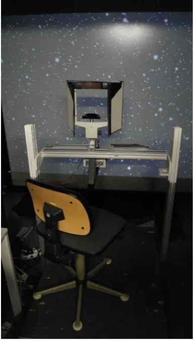
3D-glasses (NVIDIA 3D Vision Pro LCD shuttered glasses). The resulting setup filled a field of view of around 90° horizontally by 50° vertically. During the experiment, participants’ heads were stabilized using a chin rest. The view of the participants was masked so that only the screen and devices for response collection were visible. A fixation cross was not
implemented because it would lead to relative motion. As a result, people would be able to track certain elements of the scene, thus altering the nature of the task.
[image:11.595.206.399.255.594.2]Heading estimates of participants were collected using a physical pointer device. The pointer device consisted of a stainless steel rod of about 15 cm, which was connected to a potentiometer. Participants held the rod at one end and aligned the other end with the
perceived heading (Figure 3). The rod could be freely rotated on the horizontal plane and provided a < 0.1° resolution. Vection ratings were collected using a numerical keypad (Figure 3).
Stimuli
The stimuli simulated linear translation (i.e., motion in a straight line) in the horizontal plane with different headings. Heading direction and properties of the visual stimuli varied across trials.
[image:12.595.201.392.159.500.2]FOV varied between full view and a restricted view. For the restricted view, the edges of the simulation were masked resulting in a FOV of 45° horizontal by 50° vertical. The stimuli were either presented monoscopically or stereoscopically using active 3D glasses.
Participants wore the glasses throughout the whole experiment. Translation either had a motion profile with constant velocity or a variable motion profile featuring acceleration and deceleration. The constant motion profile had a velocity of 0.075 m/s. The variable motion profile had a raised cosine bell in velocity which can be specified as
v =𝑣𝑣𝑣𝑣𝑣𝑣𝑣𝑣2 (1−cos𝜔𝜔𝜔𝜔)
In each experimental condition, heading was varied as a covariate. Headings were sampled from the range of possible headings (±180°) in 16 evenly spaced steps (22.5°), starting at -168.75° (11.25°, 33.75°, 56.25°, etc.). In this way, the cardinal axes were omitted from the experiment. This was necessary because bias is not defined for the cardinal axes. Positive angles (11.5°) represented clockwise or right directions and negative angles (-11.5°) represented counter-clockwise or left directions.
Procedure
Prior to participation, potential participants were informed about the experimental goals and procedures. If the participants provided their written informed consent, they were seated in the simulator and asked to place their head on a chin rest. Once seated, they were familiarized with the setup. Practice trials were conducted to ensure their understanding of the task and to familiarize them with the procedure. Order of conditions and headings in the practice trials was identical for all participants. During the actual trials, conditions and headings were presented in randomized order. Participants were tasked to provide their heading estimates and vection ratings at the end of the trial as accurately as possible. After confirming their responses by button press, they could initiate the next trial via another button press. Every combination of a particular experimental condition and heading angle was repeated 3 times. This resulted in 16 (combinations of conditions) x 16 (headings) x 3 (repetitions) = 768 trials. Trials were measured in two different sessions on different days to ensure alertness and minimize participant burden. The experiment sessions took 90 minutes each. At the end of the experiment, participants were thanked and debriefed.
Data Analysis
Bias was calculated as angular error from heading judgments and actual headings, by calculating how many degrees the heading judgements deviated from the actual headings (heading response – stimulus heading). Vection was measured on a 7-point scale (‘1’ = no feeling of self-motion, ‘7’ = very strong feeling of self-motion). The effects of the
measured indicator for all analyzed variables. The benefit of SEM is the ability to estimate whole models with multiple dependencies in a single analysis. Path analysis was conducted in R (R Foundation for Statistical Computing, Vienna, Austria, version 3.4.1) using the lavaan package (Rosseel, 2012, version 0.5-23.1097). R script used for path analysis can be found in the appendix.
Results
[image:16.595.52.522.377.711.2]Datasets of three participants were excluded from the analysis due to technical errors with the input and saving of responses during the experiment. The remaining 17 datasets went into the analysis. Heading responses varying more than 90° from stimuli headings were treated as outliers and omitted from analysis.
Overall heading responses are shown in Figure 5. Heading errors of all participants were mapped on the y-axis across stimuli headings shown during the experiment on the x-axis, this way showing the variance of heading errors for every stimulus heading. Overall, the data indicates a bias away from the fore-aft axis with participants generally overestimating heading angles. The whole bias curve is slightly offset, thus not crossing the cardinal axes. Furthermore, the bias for backward headings seems slightly stronger than the bias for forward headings. Mean error ranged from -0.6° (for 11.25°) to -8.46 (for 146.25°).
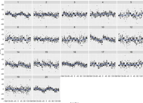
Heading responses on the individual level are shown in Figure 6. Heading errors for single participants were again mapped on the y-axis across stimuli headings shown during the experiment on the x-axis. Bias away from the fore-aft axis is also visible on the participant level - quite saliently for some participants (1,10,14,16,20) and with more noise for others (2,3,6,10,14,15,17,19). The remaining participants show different patterns with some
[image:18.595.56.531.262.626.2]considerable noise (4,5,7,8,12,18). The confidence intervals visible in Figure 6 display some substantial variance in responses of these participants.
Figure 7 again shows overall heading errors, now split by the different conditions of visual properties: FOV, disparity, profile, and scene. Bias away from the fore-aft axis can be found across all conditions, although with some differences in magnitude. The two motion profiles (constant velocity vs. raised cosine velocity) do not differ visibly with regards to the angular error. For FOV and scene, a small effect is visible in the amplitude of the curve. When FOV is restricted or when a dot cloud is shown as a scene, the bias away from the fore-aft axis is slightly stronger in magnitude. The strongest effect seems to appear for disparity: When stimuli were shown monoscopically (i.e., without disparity) participants overestimated heading direction considerably in comparison to when stimuli were shown stereoscopically.
Path analysis was used to quantify possible effects of these factors on heading estimation bias. The model specified in the beginning (Figure 1) was adjusted for the
analysis: The four visual properties, vection ratings, and angular error went into the analysis. Angular error was used as an indicator for bias. Direction of stimuli headings was added as a covariate to account for the direction sensitivity of the bias. Furthermore, the model was extended with product terms for interaction effects between the direction of stimuli headings and each of the four visual properties. Interaction terms were added to account for the sine-wave form of the bias curve: As the curve potentially inverts, effects of a factor could change depending on the direction of heading.
That means model-implied covariances are close to the actual calculated covariances from the sample, indicating that relationships specified in the model can be found in the sample. This allows to assume that visual characteristics somehow affected bias and vection. Root Mean Square Error (RMSEA) had a confidence interval from 0 to 0.02 and a p of close fit < 0.001, thus indicating a close-fitting model. The Comparative Fit Index (CFI) had a value of 0.99 and the Standardized Root Men Square Residual (SRMR) a value of 0.01. All measures of fit equally indicate a very good model fit, showing that on average model corresponds to the data. However, the model still explains very little variance found in the data, only 2% of the variance in bias (R² = 0.02) and 6% of the variance in vection (R² = 0.06). Subsequent local fit testing was conducted with multiple regression analyses to examine individual parts of the model (Table 1).
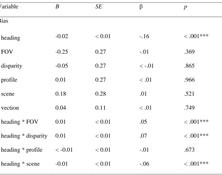
[image:20.595.77.517.426.771.2]Table 1
Summary of local fit testing done via multiple regression analyses.
Variable B SE β p
Bias
heading -0.02 < 0.01 -.16 < .001***
FOV -0.25 0.27 -.01 .369
disparity -0.05 0.27 < -.01 .865
profile 0.01 0.27 < .01 .966
scene 0.18 0.28 .01 .521
vection 0.04 0.11 < .01 .749
heading * FOV 0.01 < 0.01 .05 < .001***
heading * disparity 0.01 < 0.01 .07 < .001*** heading * profile < -0.01 < 0.01 -.01 .673
Vection
FOV 0.13 0.02 .05 < .001***
disparity -0.07 0.02 -.03 .001**
profile 0.16 0.02 .06 < .001***
scene -0.61 0.02 -.23 < .001***
The regression analyses show that the effects of the visual properties alone on bias were not significant. However, the effects of stimulus heading and the interactions between stimulus heading and FOV, disparity, and scene were significant. Bias was largely dependent on stimulus heading. Follow up analyses on simple effects of interactions were not available and were thus interpreted via figures. As can be seen in Figure 7, panels a, b, d, the blue and red line for different levels of FOV, disparity and scene differed most for heading angles exactly between cardinal axes (i.e., 45°, 135°). Headings closer to straight ahead or sideways were less influenced by any visual properties. For FOV, smaller FOV seemed to cause a larger bias, indicated by the larger amplitude of the curve. Similarly, monoscopic display for disparity and dot cloud for scene led to a larger bias. Because only certain heading angles seem to be affected, regression estimates of the effects are all quite small. Additionally, vection had no significant effect on bias, but was affected by all visual properties. As
expected larger FOV, variable motion profile and ground plane lead to higher vection ratings. Different than expected monoscopic display led to higher vection ratings.
Discussion
study could thus not be explained by visual properties alone. The visual properties only marginally affected the magnitude of bias, not its direction. FOV, disparity, and scene slightly affected heading estimates. However, as bias is direction sensitive, this effect was dependent on stimulus directions. FOV, disparity and scene increased bias in certain conditions. When participants had to judge heading angles exactly between cardinal axes, visual properties had their largest effect. Participants showed a slightly larger bias when their FOV was restricted. With a smaller FOV, more FOEs fell out of the view of the participants, making it necessary for them to estimate the direction of heading by triangulation and thus potentially leading to more errors (Koenderink & Van Doorn, 1987). Although not related to FOV, larger errors during backwards motion most likely also stem from triangulation errors. As FOE is not visible during backwards motion, participants have to solely rely on flow triangulation, thus potentially making more errors.
Despite these visible effects, there was still considerable noise in the data. Some stimuli headings or combinations of factors apparently led to substantial variance in the responses of some participants. For example, one participant (5) estimated heading direction on some trials in the direct opposite direction as stimulus heading, depending on the scene during some of the trials. This participant most likely changed strategies in heading estimation and judged dot motion instead of self-motion. As self-motion was the opposite direction as dot motion, heading responses are therefore also reversed. This led to larger heading errors and potentially skewed bias. Although no such clear pattern was visible for other participants, it is still possible that participants changed strategies between trials, leading to some variance in their responses.
during piloting, the stereoscopic stimuli were reported as compelling and vection-inducing. It is also possible that the vection ratings for some participants do not directly reflect the
experience of vection and some different concept was rated instead. During practice trials, some participants reported that they had erroneously rated speed instead of vection. Although these participants were corrected and the majority of participants seemingly understood the concept of vection. Additionally, as earlier research has shown, longer durations are needed for linear motion to give the impression of vection (Dichgans & Brandt, 1978). The fact that vection generally has onset times that exceed the duration of the visual motion stimuli presented in the current study may explain why vection was not found to affect bias.
Rejecting the model despite a good model fit in the analyses seems counterintuitive, but good fit has to be taken with a grain of salt because of several reasons. First, as bias is direction sensitive, adding stimuli headings to the analysis most likely largely improved model fit. Thus, visual properties potentially have only a small role in the model fit calculated. Nevertheless, stimuli headings have to be included to account for direction sensitivity of bias. Second, the model in the analysis is just one plausible model with further equivalent models. In the field of SEM, equivalent models are models with the same
shortcoming is often criticized in SEM literature because nested structure of data is rarely considered (Julian, 2001). A multilevel analysis of data would be a viable approach to counter this issue but during the time of the study, it was not available in lavaan and because it can be considered an advanced technique in SEM (Marcoulides & Schumacker, 1996) it went beyond the scope of this study.
Similarly, the experimental setup could have impacted the overall bias. Using a dial to indicate heading is somewhat artificial and could thus have affected the reference points of the participants and their internal representation of the heading. Additionally, the task of pointing a dial includes a motoric and haptic component, possibly affecting bias. However, Crane (2012) compared responses to spoken heading stimuli with responses to visual and vestibular stimuli and could show that bias mostly stems from sensory stimuli rather than haptic or motor influences. The fact that visual properties affected bias to a certain degree in the present study likewise shows that bias more likely stems from sensory stimuli.
Additionally, studies using on screen arrows or probes (Hummel et al., 2016; Li et al., 2002) or head pointing (Telford et al., 1995) as response mode also found similar biases. Thus, we assume that the experimental setup did not affect bias systematically.
al., 2010). It is further possible that the distribution of preferred directions of neural populations in the MSTd varies across individuals, leading to individually different biases (De Winkel et al., 2017).
References
Andersen, G. J., & Braunstein, M. L. (1985). Induced self-motion in central vision. Journal
of Experimental Psychology: Human Perception and Performance, 11, 122–132.
doi:10.1037/0096-1523.11.2.122
Banks, M. S., Ehrlich, S. M., Backus, B. T., & Crowell, J. A. (1996). Estimating heading
during real and simulated eye movements. Vision Research, 36, 431–443.
doi:10.1016/0042-6989(95)00122-0
Bollen, K. A. (1989). Structural equations with latent variables. New York, NY: Wiley.
Brandt, T., Wist, E. R., & Dichgans, J. (1975). Foreground and background in dynamic
spatial orientation. Attention, Perception, & Psychophysics, 17, 497–503.
doi:10.3758/BF03203301
Butler, J. S., Campos, J. L., & Bülthoff, H. H. (2015). Optimal visual–vestibular integration
under conditions of conflicting intersensory motion profiles. Experimental Brain
Research, 233, 587–597. doi:10.1007/s00221-014-4136-1
Butler, J. S., Smith, S. T., Campos, J. L., & Bülthoff, H. H. (2010). Bayesian integration of
visual and vestibular signals for heading. Journal of Vision, 10(11), 1–13. doi:
10.1167/10.11.23
Crane, B. T. (2012). Direction specific biases in human visual and vestibular heading
Perception. Plos ONE, 7(12), 1–15. doi:10.1371/journal.pone.0051383
Crane, B. T. (2014). Human visual and vestibular heading perception in the vertical planes.
Journal of the Association for Research in Otolaryngology, 15, 87–102.
doi:10.1007/s10162-013-0423-y
Crowell, J. A., & Banks, M. S. (1993). Perceiving heading with different retinal regions and
types of optic flow. Attention, Perception, & Psychophysics, 53, 325–337.
Cuturi, L. F., & MacNeilage, P. R. (2013). Systematic biases in human heading perception.
Plos ONE, 8(2), 1–11. doi:10.1371/journal.pone.0056862
D’Avossa, G., & Kersten, D. (1996). Evidence in human subjects for independent coding of
azimuth and elevation for direction of heading from optic flow. Vision Research, 36,
2915–2924. doi:10.1016/0042-6989(96)00010-7
De Winkel, K. N., Grácio, B. J. C., Groen, E. L., & Werkhoven, P. (2010). Visual inertial
coherence zone in the perception of heading. In AIAA Modeling and Simulation
Technologies Conference 2010 (pp. 7916–7922). doi:10.2514/6.2010-7916
De Winkel, K. N., Katliar, M., & Bülthoff, H. H. (2015). Forced fusion in multisensory
heading estimation. Plos ONE, 10, 1–20. doi:10.1371/journal.pone.0127104
De Winkel, K. N., Katliar, M., & Bülthoff, H. H. (2017). Causal inference in multisensory
heading estimation. Plos ONE, 12, 1–20. doi:0.1371/journal.pone.0169676
De Winkel, K. N., Weesie, J., Werkhoven, P. J., & Groen, E. L. (2010). Integration of visual
and inertial cues in perceived heading of self-motion. Journal of Vision, 10(12):1, 1–
10. doi:10.1167/10.12.1
Dichgans, J., & Brandt, T. (1978). Visual-vestibular interaction: Effects on self-motion
perception and postural control. In R. Held, H. W. Leibowitz, & H. L. Teuber (Eds.)
Handbook of sensory physiology Vol. VIII (pp. 756–804). New York, NY: Springer
Verlag.
Fetsch, C. R., Turner, A. H., DeAngelis, G. C., & Angelaki, D. E. (2009). Dynamic
reweighting of visual and vestibular cues during self-motion perception. Journal of
Neuroscience, 29, 15601–15612. doi:10.1523/JNEUROSCI.2574-09.2009
Gibson, J. J. (1950). The perception of the visual world. Cambridge, MA: The Riverside
Grigo, A., & Lappe, M. (1998). Interaction of stereo vision and optic flow processing
revealed by an illusory stimulus. Vision Research, 38, 281–290.
doi:10.1016/S0042-6989(97)00123-5
Gu, Y., DeAngelis, G. C., & Angelaki, D. E. (2007). A functional link between area MSTd
and heading perception based on vestibular signals. Nature Neuroscience, 10, 1038–
1047. doi:10.1038/nn1935
Gu, Y., Fetsch, C. R., Adeyemo, B., DeAngelis, G. C., & Angelaki, D. E. (2010). Decoding
of MSTd population activity accounts for variations in the precision of heading
perception. Neuron, 66, 596–609.doi:10.1016/j.neuron.2010.04.026
Habak, C., Casanova, C., & Faubert, J. (2002). Central and peripheral interactions in the
perception of optic flow. Vision Research, 42, 2843–2852.
doi:10.1016/S0042-6989(02)00355-3
Howard, I. P. (1982). Human visual orientation. Hoboken, NJ: John Wiley & Sons.
Hummel, N., Cuturi, L. F., MacNeilage, P. R., & Flanagin, V. L. (2016). The effect of supine
body position on human heading perception. Journal of Vision, 16(3):19, 1–11.
doi:10.1167/16.3.19
Johnston, I. R., White, G. R., & Cumming, R. W. (1973). The role of optical expansion
patterns in locomotor control. The American Journal of Psychology, 86, 311–324.
doi:10.2307/1421439
Julian, M. W. (2001). The consequences of ignoring multilevel data structures in
nonhierarchical covariance modeling. Structural Equation Modeling, 8, 325–352.
doi:10.1207/S15328007SEM0803_1
Koenderink, J. J., & Van Doorn, A. J. (1987). Facts on optic flow. Biological Cybernetics,
Lappe, M., Bremmer, F., & Van Den Berg, A. V. (1999). Perception of self-motion from
visual flow. Trends in Cognitive Sciences, 3, 329–336.
doi:10.1016/S1364-6613(99)01364-9
Li, L. I., Peli, E., & Warren, W. H. (2002). Heading perception in patients with advanced
retinitis pigmentosa. Optometry & Vision Science, 79, 581–589. doi:
10.1097/00006324-200209000-00009
MacNeilage, P. R., Banks, M. S., Berger, D. R., & Bülthoff, H. H. (2007). A Bayesian model
of the disambiguation of gravitoinertial force by visual cues. Experimental Brain
Research, 179, 263–290. doi:10.1007/s00221-006-0792-0
Marcoulides, G. A., & Schumacker, R. E. (Eds.). (1996). Advanced structural equation
modeling: Issues and techniques. Mahwah, NJ: Lawrence Erlbaum Associates Inc..
Nakamura, S., & Shimojo, S. (1999). Critical role of foreground stimuli in perceiving
visually induced self-motion (vection). Perception, 28, 893–902. doi:10.1068/p2939
Palmisano, S. A. (1996). Perceiving self-motion in depth: the role of stereoscopic motion and
changing-size cues. Perception and Psychophysics, 58, 1168–1176.
doi:10.3758/BF03207550
Palmisano, S. A. (2002). Consistent stereoscopic information increases the perceived speed
of vection in depth. Perception, 31, 463–480. doi:10.1068/p3321
Palmisano, S. A., Allison, R. & Pekin, F. (2008). Accelerating self-motion displays produce
more compelling vection in depth. Perception, 37, 22–33. doi:10.1068/p5806
Pretto, P., Ogier, M., Bülthoff, H. H., & Bresciani, J. P. (2009). Influence of the size of the
field of view on motion perception. Computers & Graphics, 33, 139–146.
doi:10.1016/j.cag.2009.01.003
Riecke, B. E., Schulte-Pelkum, J., Avraamides, M. N., Heyde, M. V. D., & Bülthoff, H. H.
reality. ACM Transactions on Applied Perception (TAP), 3, 194–216.
doi:10.1145/1166087.1166091
Rosseel, Y. (2012). Lavaan: An R package for structural equation modeling. Journal of
Statistical Software, 48(2), 1–36.
Royden, C. S., Banks, M. S., & Crowell, J. A. (1992). The perception of heading during eye
movements. Nature, 360, 583–585.
Saito, H.A., Yukie, M., Tanaka, K., Hikosaka, K., Fukada, Y., & Iwai, E. (1986). Integration
of direction signals of image motion in the superior temporal sulcus of the macaque
monkey. Journal of Neuroscience, 6, 145–157.
Stelzl, I. (1986). Changing a causal hypothesis without changing the fit: Some rules for
generating equivalent path models. Multivariate Behavioral Research, 21, 309–331.
doi:10.1207/s15327906mbr2103_3
Telford, L., & Howard, I. P. (1996). Role of optical flow field asymmetry in the perception of
heading during linear motion. Perception & Psychophysics, 58, 283–288.
doi:10.3758/BF03211881
Telford, L., Howard, I. P., & Ohmi, M. (1995). Heading judgments during active and passive
self-motion. Experimental Brain Research, 104, 502–510. doi:10.1007/BF00231984
Trutoiu, L. C., Mohler, B. J., Schulte-Pelkum, J., & Bülthoff, H. H. (2009). Circular, linear,
and curvilinear vection in a large-screen virtual environment with floor projection.
Computers & Graphics, 33, 47–58.doi:10.1016/j.cag.2008.11.008
Van Den Berg, A. V., & Brenner, E. (1994a). Humans combine the optic flow with static
depth cues for robust perception of heading. Vision Research, 34, 2153–2167.
doi:10.1016/0042-6989(94)90324-7
Van Den Berg, A. V., & Brenner, E. (1994b). Why two eyes are better than one for
Warren, R. (1976). The perception of egomotion. Journal of Experimental Psychology:
Human Perception and Performance, 2, 448–456. doi:10.1037/0096-1523.2.3.448
Warren, W. H., & Hannon, D. J. (1988). Direction of self-motion is perceived from optical
flow. Nature, 336, 162–163. doi:10.1038/336162a0
Warren, W. H., & Kurtz, K. J. (1992). The role of central and peripheral vision in perceiving
the direction of self-motion. Perception & Psychophysics, 51, 443–454.
doi:10.3758/BF03211640
Warren, W. H., Morris, M. W., & Kalish, M. (1988). Perception of translational heading from
optical flow. Journal of Experimental Psychology: Human performance perception
and performance, 14, 646–660. doi:10.1037/0096-1523.14.4.646
Ziegler, L. R., & Roy, J. P. (1998). Large scale stereopsis and optic flow: depth enhanced by
speed and opponent-motion. Vision Research, 38, 1199–1209.
Appendix
R Script
Import datset
# Import dataset from csv file
data <- read.csv(file = "D:/Dokumente/Studium/Universiteit Twente/Thesis/An
alysis/Data/dataset.csv")
Prepare dataset
library(dplyr)
##
## Attaching package: 'dplyr'
## The following objects are masked from 'package:stats':
##
## filter, lag
## The following objects are masked from 'package:base':
##
## intersect, setdiff, setequal, union
# Add session counter
data$sess <- ifelse(data$trial <= 384, 1, 2)
# Add trial counter
data <- data %>%
group_by(par,FOV,disparity,profile,scene,theta) %>%
mutate(rep = row_number())
Filter excluded datasets
# Filter out participants
data <- data %>% filter(par != 11) # Error saving responses of second sessi
on
data <- data %>% filter(par != 13) # Error during pointer initialization
data <- data %>% filter(par != 9) # Error saving vection ratings of first s
ession
data <- data %>% filter(vection > 0)
Outlier handling
# Filter heading judgements
data <- data %>% filter(error <= 90 & error >= -90)
Create dummy variables for interaction
# Interaction between factors and theta
data$"thetaFOV" = data$FOV*data$theta
data$"thetadisparity" = data$disparity*data$theta
data$"thetaprofile" = data$profile*data$theta
data$"thetascene" = data$scene*data$theta
Define path models
# Full model with interactions
path.full <-'
error ~ theta + FOV + disparity + profile + scene + vection +
thetaFOV + thetadisparity + thetaprofile + thetascene
vection ~ FOV + disparity + profile + scene'
Calculate model fit
library(lavaan)
## This is lavaan 0.5-23.1097
## lavaan is BETA software! Please report any bugs.
model.full <- sem(path.full, data, warn = TRUE, estimator = "mlr", meanstru
cture = TRUE)
summary(model.full, standardized = TRUE, fit.measures = TRUE, rsquare = TRU
E)
## lavaan (0.5-23.1097) converged normally after 79 iterations
##
## Number of observations 12551
##
## Estimator ML Robust
## Degrees of freedom 5 5
## P-value (Chi-square) 0.133 0.124
## Scaling correction factor 0.976
## for the Yuan-Bentler correction
##
## Model test baseline model:
##
## Minimum Function Test Statistic 1035.871 1031.718
## Degrees of freedom 19 19
## P-value 0.000 0.000
##
## User model versus baseline model:
##
## Comparative Fit Index (CFI) 0.997 0.996
## Tucker-Lewis Index (TLI) 0.987 0.986
##
## Robust Comparative Fit Index (CFI) 0.996
## Robust Tucker-Lewis Index (TLI) 0.987
##
## Loglikelihood and Information Criteria:
##
## Loglikelihood user model (H0) -454911.236 -454911.236
## Scaling correction factor 1.050
## for the MLR correction
## Loglikelihood unrestricted model (H1) -454907.013 -454907.013
## Scaling correction factor 1.034
## for the MLR correction
##
## Number of free parameters 18 18
## Akaike (AIC) 909858.472 909858.472
## Bayesian (BIC) 909992.348 909992.348
## Sample-size adjusted Bayesian (BIC) 909935.146 909935.146
##
## Root Mean Square Error of Approximation:
##
## 90 Percent Confidence Interval 0.000 0.016 0.000 0.01 6
## P-value RMSEA <= 0.05 1.000 1.000
##
## Robust RMSEA 0.008
## 90 Percent Confidence Interval 0.000 0.01 6
##
## Standardized Root Mean Square Residual:
##
## SRMR 0.005 0.005
##
## Parameter Estimates:
##
## Information Observed
## Standard Errors Robust.huber.white
##
## Regressions:
## Estimate Std.Err z-value P(>|z|) Std.lv Std.a ll
## error ~
## theta -0.023 0.003 -7.843 0.000 -0.023 -0.1 55
## FOV -0.246 0.274 -0.898 0.369 -0.246 -0.0 08
## disparity -0.046 0.274 -0.170 0.865 -0.046 -0.0 02
## profile 0.012 0.274 0.043 0.966 0.012 0.0 00
## scene 0.181 0.282 0.642 0.521 0.181 0.0 06
## vection 0.036 0.111 0.320 0.749 0.036 0.0 03
## thetaFOV 0.010 0.003 3.801 0.000 0.010 0.0 48
## thetadisparity 0.014 0.003 5.414 0.000 0.014 0.0 68
## thetaprofile -0.001 0.003 -0.422 0.673 -0.001 -0.0 05
## thetascene -0.013 0.003 -5.058 0.000 -0.013 -0.0 63
## FOV 0.127 0.023 5.576 0.000 0.127 0.0 48
## disparity -0.074 0.023 -3.218 0.001 -0.074 -0.0 28
## profile 0.155 0.023 6.793 0.000 0.155 0.0 59
## scene -0.608 0.023 -26.612 0.000 -0.608 -0.2 30
##
## Intercepts:
## Estimate Std.Err z-value P(>|z|) Std.lv Std.a ll
## .error -2.238 0.511 -4.381 0.000 -2.238 -0.1 45
## .vection 3.627 0.025 143.581 0.000 3.627 2.7 47
##
## Variances:
## Estimate Std.Err z-value P(>|z|) Std.lv Std.a ll
## .error 234.713 4.057 57.847 0.000 234.713 0.9 80
## .vection 1.639 0.020 83.340 0.000 1.639 0.9 40
##
## R-Square:
## Estimate
## error 0.020