Determining design relations for a magneto caloric device with multiple magneto caloric materials using numerical software

UNIVERSITY OFTWENTE

FACULTY OFENGINEERINGTECHNOLOGY LABORATORY OFTHERMALENGINEERING

Master’s Thesis

Determining design relations for a magnetocaloric device with

multiple magneto caloric materials using numerical software.

Author

C.P.J. Ridderhof

Supervisors

prof.dr.ir. Th.H. van der Meer

dr.ir. G.G.M. Stoffels

dr.ir. Mina Shahi

Exam committe

prof.dr.ir. Th.H. van der Meer

prof.dr.ir. M. ter Brake

dr.ir. G.G.M. Stoffels

dr.ir. Mina Shahi

PREFACE

With the health of the earthly environment high on the public agenda, conventional heating and cooling techniques are in need of replacing due to efficiency and environmental reasons. Active heat transfer will be done differently, more eco-friendly, in the near future. The magnetocaloric effect may be at the foundation of a new heat pump. In order to create an economical feasible heat pump significant improvements have to be made concerning the total heat transfer coefficient.

This thesis represents the work I did as my master assignment for the department of mechanical engineering, at the faculty of thermodynamic engineering at the Twente University. The main purpose of my assignment was to further investigate the magneto caloric effect and develop a 2D model of the AMR. This model was already initiated by Jöran Stoter a previous master student. The model needed further improvements and validation. Next to this the use of a different materials has been implemented. Materials developed by the department of material sciences of TU Delft have been used.

I would like to express my sincere gratitude to my supervisors: professor van der Meer and doctor Stoffels. I always felt motivated to continue to work on the thesis. I hope this work provides a contribution to the research of eco-friendly heat pumps,

SUMMARY

This thesis describes the research into the magneto caloric effect(MCE) and the use of it in a regenerative setting, or active magneto regenerator(AMR). The MCE is first described with thermodynamics. From previous research at the Twente University it seems that the energy balance as found in the thermodynamics does not hold up. The thermodynamics found are tested in a 0D-model. This means only the temporal domain will be used. The thermo-dynamics are implemented into a model in Matlab. When using a small enough time-step the energy balance does hold up. It can be concluded that the thermodynamics are validated. In order to describe the MCE the material properties are of great importance. They are described with the use of the ’Mean Field Theory’(MFT).

In the second part of the thesis a 2D model of an AMR is created with gadolinium as magneto caloric material (MCM). This model is made with the software program Comsol Multi-physics. At first a mesh study is performed looking for an optimal spatial and temporal resolution where the computational time is kept at reasonable lengths. In order to prove that the model is representative, two validation methods are used. At first a quasi analytical solution is used to validate the cooling capacity. This also provides for feedback concerning the energy balance. The second validation uses data as found in literature. The model is given the same dimensions as provided by literature. The model provides the same behaviour at various utilization factors as found in literature. However the magnitude varies greatly: the model does not include a heat-loss model apparently.

To engineer a heat pump capable of handling larger temperature differences other MCM is required than gadolin-ium. The third part of this thesis describes the numerical research into the so-called Brück materials named after one of the founding fathers of this material. This material can be used as MCM due to its giant magneto caloric effect whilst retaining optimal material properties such as minimal hysteresis or physical deformations. The Curie temperature of this material can be changed by altering the composition. The literature describes various material families and for this thesis the Mn1.25Fe0.7P1−ySiyfamily is used, where y = 0.49, 0.50, 0.51 or 0.52. The Curie

tem-peratures are from lower to higher values respectively. The new 2D-model describes these material as placed next to each other in successive Curie temperature. The material properties are derived from literature.

SAMENVATTING

Deze thesis beschrijft het onderzoek naar het magneto calorisch effect en het gebruik ervan in een regeneratieve opstelling ook wel actief magnetische regenerator (AMR) genoemd. Hiertoe wordt eerst het magneto calorisch ef-fect beschreven in een thermodynamische afleiding. In vorige onderzoeken aan de Twente University blijkt dat de energiebalans niet intact is. Hiertoe wordt de beschreven thermodynamische afleiding getoetst in een 0D-setting. Dat wil zeggen dat er gebruik gemaakt wordt van een domein in de temporele ruimte. Het model is geïmple-menteerd in Matlab en het blijkt dat bij een afdoende kleine tijdstap alle beschreven energieà ´nn elkaar opheffen en daardoor kan geconcludeerd worden dat de thermodynamica gevalideerd blijkt. Om het magneto calorische effect te beschrijven zijn de materiaaleigenschappen van belang. De materiaaleigenschappen van gadolinium worden beschreven door de zogenaamde ’Mean Field Theory’.

In het tweede deel wordt een 2D model van een AMR beschreven. Dit model is gemaakt in het softwarepakket COMSOL. Als eerste wordt er gekeken welke spatiele en temporele resoluties stabiele resultaten geven. Het blijkt dat binnen acceptabele rekentijden stabiele resultaten kunnen worden gehaald. Om het model van enige zingeving te voorzien wordt een quasi analytische afleiding gedaan van het magneto calorische effect, waarna wordt gekeken of het model dezelfde uitkomst geeft. Om het model verder te valideren wordt gebruik gemaakt van in literatuur gevonden karakteristieken. De dimensionalisering wordt gedaan aan de hand van in dezelfde literatuur beschreven experimenten. Het blijkt dit 2D model hetzelfde gedrag beschrijft als gevonden in literatuur. Eén verschil is over-duidelijk aanwezig: het model omvat geen geïmplementeerd warmte-verlies-model.

Om een warmtepomp te maken die een groter temperatuurbereik aan kan moet er gekeken worden naar andere materialen dan gadolinium. Het derde deel van deze master thesis beschrijft het numerieke onderzoek naar een zogenaamd Brück materiaal in een 2D model. Deze naam is afgeleid naar de naam van de onderzoeksgroep leider: prof. Brück. Dit materiaal verdient de aandacht omdat het materiaal een groot magneto calorisch effect ondergaat bij het opleggen van een magneetveld. Daarbij kan het materiaal worden aangepast om bij de heersende temper-aturen een groot MCE te laten zien. De literatuur beschrijft verschillende materiaal families die dergelijke effecten laten zien, voor deze thesis wordt gebruik gemaakt van de Mn1.25Fe0.7P1−ySiy familie, waar y = 0.49,0.50,0.51 of

0.52 kan zijn. De Curie temperaturen volgen elkaar respectievelijk op. Het volgende 2D model omvat deze mate-rialen naast elkaar geplaatst in opvolgende Curie temperatuur. De materiaaleigenschappen zijn afgeleid uit de lit-eratuur. Uit de gevonden materiaaleigenschappen blijkt dat het magneto calorische effect de warmte die vrijkomt als gevonden in de literatuur niet beschrijft. Er blijk sprake te zijn van zogenaamde latente warmte die vrijkomt bij de overgang van de ferromagnetische toestand naar de paramagnetische. Om dit verschil op te vangen wordt de afgeleide van de interne magnetisatie curve versterkt. Verder blijkt dat door een asymmetrie in de warmtecapaciteit dat het materiaal zich beter leent in een opstelling waar een koude warmtebron is opgesteld tegen over een warm koellichaam. Om dit aan te tonen wordt een studie gedaan naar de maximale temperatuur spanne bij verschil-lende utilisatie factoren. Deze studie wordt tweemaal gedaan. In eerste instantie wordt de koude warmtewisselaar op constante temperatuur gehouden en in de tweede wordt de warme warmtewisselaar op constante temperatuur gehouden. Het blijkt met de koude warmtewisselaar op constante temperatuur een groter temperatuurspanne kan worden opgebouwd in vergelijking met de warme warmtewisselaar.

CONTENTS

Preface i

Summary iii

Samenvatting v

1 Introduction 1

1.1 Heat pumps . . . 1

1.2 The magnetocaloric effect . . . 1

1.3 Active Magnetic Regenerator . . . 2

2 Fundamentals of the magnetocaloric effect 5 2.1 Introduction . . . 5

2.2 Energy . . . 5

2.2.1 Isothermal entropy change . . . 6

2.2.2 Adiabatic temperature change . . . 7

2.3 Cyclic operation . . . 8

3 Material properties 9 3.1 Transition Temperature TC . . . 9

3.1.1 1stand 2ndorder transitions . . . 9

3.2 Material properties of Gadolinium . . . 9

3.3 The Weiss Mean Field Model . . . 10

3.4 The Debye & Sommerfeld model . . . 11

3.5 Theoretical material properties . . . 11

3.5.1 Heat Capacity . . . 11

3.5.2 Magnetization . . . 11

3.5.3 Temperature derivative of magnetization with respect to temperature . . . 12

3.6 Material Properties of Mn1.25Fe0.7P1−ySiy . . . 13

3.6.1 Heat capacity . . . 13

3.6.2 Magnetization . . . 16

3.6.3 Density and thermal conductivity . . . 17

4 0D-Model 19 4.1 Model set up . . . 19

4.1.1 Numerical Implementation . . . 19

4.1.2 Modelling the magnetic field . . . 20

4.2 Results and Discussion . . . 22

4.2.1 Temporal Study . . . 23

5 Active magnetic Regenerator 25

5.1 2D model - Gadolinium . . . 25

5.2 Model Design . . . 27

5.2.1 The convective Term . . . 28

5.2.2 Input parameters . . . 28

5.2.3 Mesh and Time stepping . . . 29

5.3 Validation . . . 31

5.4 Results . . . 32

5.5 Discussion . . . 32

6 2D model - Mn1.25Fe0.7P1−ySiy-AMR 35 6.1 Introduction . . . 35

6.2 Experiments . . . 36

6.3 Results . . . 37

6.3.1 0D Temperature experiments . . . 37

6.3.2 2D Utilization experiments . . . 38

6.4 discussion . . . 42

7 Conclusion and Discussion 43 7.1 0D model . . . 43

7.2 2D model - Gadolinium . . . 43

7.3 2D model - Mn1.25Fe0.7P1−ySiy . . . 43

7.3.1 Recommendation: 2.5D model . . . 44

7.3.2 Recommendation: Utilization factor . . . 44

Bibliography I

Nomenclature III

0D model figures V

CHAPTER

ONE

INTRODUCTION

1.1

H

EAT PUMPS

The current focus upon the human effect on climate change requires a more efficient way of heat transport. Cli-mates where both heating and cooling are required, the heat pump offers and energy-efficient way of replacing furnaces or air-conditioners. The magnetocaloric heat pump requires electricity to move heat from a cold source towards a hot sink: the refrigerator cycle. Moving heat against the temperature gradient is the soulpurpose of a heat pump.

Currently the most used heat pump relies on the vapor-compression cycle. The heat is being moved using a closed-loop cycle: compressing, condensing, expanding and evaporating a refrigerant fluid. The configuration of the system will determine whether the net effect is the cooling or heating of a specified volume. There are various reasons why this type of heat pump is dominant: it is scalable, relatively compact, has a high reliability and efficient operation at 30 to 60 % of Carnot. This system can be found in AC-units in cars or refrigerators at home.

Most of these system use fluids, called refrigerants, are harmful for the environment. Due to the great number of moving parts in such a system the durability is affected. Next to this, due to moving parts, the system can be very loud. The last reason being the relative low efficiency in comparison to promising magnetocaloric heat pumps [1] [2], [3]. Due to an increasing cooling/heating demand the impact of these systems on the energy consumption is high [4]. Therefor by investigating alternative heat-pumps the human effect on climate change could be altered in a positive way [5].

1.2

T

HE MAGNETOCALORIC EFFECT

Magnetocaloric energy conversion is a technique based upon the use of the magnetocaloric effect, or MCE for short. The occurrence of the MCE happens under the influence of a changing applied magnetic field on a ferro-magnetic material[6].

Two distinctive cases are usually described concerning the way the MCE is described: adiabatic or isothermally. In isothermal conditions the temperature is kept constant at all times whether in adiabatic conditions there is no heat transfer from or to the domain (magnetocaloric material). In the last case a temperature difference could be measured, whereas the isothermal case describes how much energy is being transferred to or from the domain.

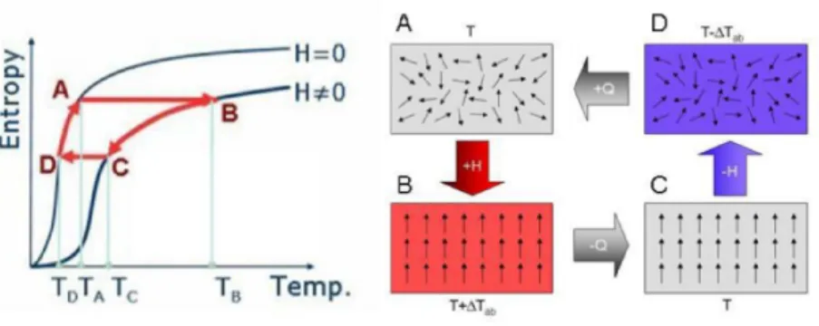
In terms of introductory knowledge the magneto caloric cycle will be explained including the adiabatic temper-ature rise. Figure 1.2.1 provides an overview of the different stages. The stages are ordered in time: Starting at A, continuing to D. Where the path from D to A may not be forgotten.

increase. This causes the atoms in the material to vibrate more intensively, with an rise in temperature as effect, point B in figure 1.2.1. The free electron entropy is not altered by the changing applied magnetic field.

Now the temperature has increased above for example the ambient temperature, the current state can be main-tained for a longer period of time. During this time period the material can cool down (not adiabatic), whilst en-during a magnetic field. This process is illustrated when moving from state B to C.

The following step in the cycle is removing the magnetic field. This in turn will increase the magnetic entropy. However, the same entropy law applies: the lattice entropy will increase and therefore the temperature of the mate-rial will drop. However, due to the heat removal the final temperature will be lower than the ambient temperature. (moving from point C to D in figure 1.2.1).

Maintaining the state of no applied magnetic field will allow the material to obtain the ambient temperature after which it reached its initial state again.

In the case of an truly adiabatic and steady state situation the temperature at the end of the cycle is the same at the beginning of the cycle. The ambient temperature or heat transfer from or to the ambient is not taken into account.

Figure 1.2.1:The magnetocaloric effect is shown here in a temperature entropy diagram and provided with

illus-trative figures to provide insight into the increase of the magnetic dipole moment.

1.3

A

CTIVE

M

AGNETIC

R

EGENERATOR

For an efficient use of the magneto caloric effect, usable temperature differences are required. Referring to the refrigerator example: an temperature difference between both sides of the refrigerator of approximately 15 Kelvin is required. Whereas the magneto caloric effect on itself can create an temperature step of approximately 5 Kelvin, depended on the magnetic field strength.

The magnetocaloric effect used in heat pumps is usually depended on permanent magnets as the magnetic field source. In order to create an high temperature span very cost intensive magnets would have to be used. These powerful magnets would create a high temperature change over one cycle. Next to this the high magnetic fields could provide mechanical challenges, which make the heat pump cost intensive again. Usually magnets, that are affordable, provide a magnetic field of 0.8 to 1.5T. These magnetic fields lead to a adiabatic temperature change in gadolinium of about 5K [7]. This temperature change is too low for the usual required temperature span which is in the order of 20 to 35 Kelvin. The most common way to obtain an higher temperature span created by a heat pump is to use a cycle that includes regeneration. The MCE must be used as an active component as suggested by Barclay in 1983 [8].

The main indicator of an active magnetic regenerator(AMR) is that all parts of the AMR simultaneously accept or reject heat to the heat transfer fluid. The fluid transport on its turns ensures the transfer of heat to internal neighbouring parts of the AMR or the heat exchangers. In order to obtain the regenerative effect a oscillatory fluid flow is applied. In this thesis a Brayton-like thermodynamic cycle will be used. A further detailed explanation will be given in chapter 5.

when using gadolinium for practical applications [9] [10] and [11]. Next to this gadolinium is an expensive material. Different materials have been investigated for their MCE. In this thesis the use of Mn1.25Fe0.7P1−ySiyas a substitute

CHAPTER

TWO

FUNDAMENTALS OF THE MAGNETOCALORIC EFFECT

The current chapter presents the thermodynamics of the magnetocaloric effect(MCE). This chapter prepares for the energy balance check, as will be presented in chapter 4. In order to obtain a proper energy balance a thorough under-standing of the thermodynamics is required.

2.1

I

NTRODUCTION

The MCE is produced by a interaction between the spin system of the material and the change of internal mag-netic field strength, H. The MCE is discovered for more than a century ago. All magmag-netic materials can produce a MCE, however, the magnitude of its effect varies strongly per material. The thermodynamics are related to the magnetocaloric material as the observed system. Therefore the magnetic field inside the magnetocaloric mate-rial is considered. The external magnetic field, related to the magnetic field source, is not considered. For this experiment volume and pressure are assumed constant.

When increasing the magnetic field strength in a soft-ferromagnet the electronic spins tend to align. The result is a, inevitably, lowering of the magnetic entropy. Depending on the boundary conditions; adiabatic or isothermal, the total entropy will decrease or remain constant. The total entropy can be written as the sum of several entropies: the magnetic, electronic and lattice entropy. The following expression as made by Pecharsky et al. 2001[13], can be found:

S=Smag+Slat+Selc (2.1.1)

Due to its reversibility it seems obvious that this effect can be used as basis for a heat pump. In the 1920 and ’30s the MCE was used in order to cool to temperatures close to the absolute zero (0.25K). This was done using a magnetic salt [14]. This thesis is primarily concerned with a magnetic heat pump at room temperature. The first experimental device using the MCE was a refrigerator presented by Brown 1976 [15].

2.2

E

NERGY

The first law of thermodynamics for a closed system states that the internal energy of the magnetocaloric material will increase if heat is added or if work is performed upon the material. This law is usually written as follows:

d u=δq−δw (2.2.1)

In order to produce the MCE the magnetocaloric material has to be moved into the magnetic field. This results in a change of the magnetic field inside the material. Due to the magnetic field the material also gets magnetized; it will start to produce its own magnetic field. The work required to magnetize the magnetocaloric material can be written as:

The system can be considered isentropic and adiabatic resulting in the following use of the second law of thermo-dynamics:

d q=T d s (2.2.3)

Rewriting 2.2.1 into:

d u=T d s+µ0H d M (2.2.4)

The derivative of the specific total entropy is defined in equation 2.2.11. The terms in this equation can be rewritten in terms of heat capacity as shown in equation 2.2.5 and 2.2.6.

cH=

µδ_q

δT

¶

H=

T

µδ_s

δT

¶

H

(2.2.5)

cT =

µδ_q

δH

¶

T=

T

µδ_s

δH

¶

T

(2.2.6) Which finally will provide a more usable term for dq:

d q₌ch(T,H)d T+cT(T,H)d H (2.2.7)

Using the following Maxwell relation the latter equation, 2.2.6, can be rewritten as: cT =T

µ

δs

δH

¶

T=µ

0T µ δM δT ¶ H (2.2.8) Now equation 2.2.7 can be rewritten as:

d q₌ch(T,H)d T+µ0T

µ δM δT ¶ H (2.2.9) Looking at equation 2.2.4 and 2.2.9 the internal energy can be rewritten as:

d u=ch(T,H)d T+µ0T

µδ_M

δT

¶

H+µ0

H d M (2.2.10)

Equation 2.2.10 will later be used as a check for the energy balance. Next to this this expression can be rewritten in to a source therm for heat, see paragraph 2.2.2.

2.2.1

I

When considering the total entropy to be a function of the magnetic field strength and temperature the following total derivative of the entropy can be found

d S(T,H)₌

µδ_S

δT

¶

H

d T₊

µδ_S

δH

¶

T

d H. (2.2.11)

The entropy change can be rewritten into: *De juiste vergelijkingen moeten nog genoemd worden

d s(T,H)=

µδ_S

δH

¶

T

d H=µ0

µδ_M

δT

¶

H

d H (2.2.12)

When the applied field varies, the internal field will also change. When considering isothermal conditions the isothermal entropy change can be defined as follows:

∆s=s2−s1=

Z H₂

H1

µδ_s

δH

¶

T

d H (2.2.13)

Using the maxwell relation, 2.2.8, equation 2.2.13 can be rewritten:

∆s₌

Z H2

H1

µ0

µδ_M

δT

¶

H

d H (2.2.14)

∆s=

Z H2

H1 cT

2.2.2

A

In order to characterize the magnetocaloric material the adiabatic temperature change will be used throughout the thesis. This means that the temperature change is caused by the change of the magnetic field in the absence of heat flow. In this type of process, the adiabatic-isentropic process, the total specific entropy does not alter. This means that equation 2.2.11 is equal to zero. Using equation 2.2.6 the following relation can be found:

µδ_s

δT

¶

H=

µδ_s

δH

¶

T=µ

0

µδ_M

δT

¶

H

d H (2.2.16)

Which can be rewritten into the expression for adiabatic temperature change, using equation 2.2.3:

∆Tad= −T µ0

cH

Z H2

H1

µδ_M

δT

¶

H

d H (2.2.17)

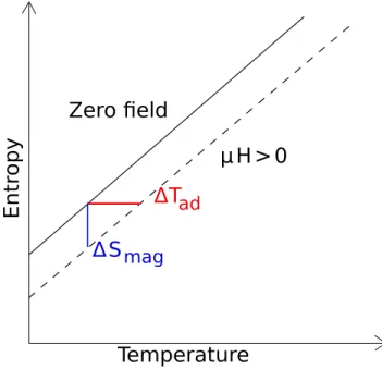
The two types of change can be represented in a T-S diagram as shown in figure 2.2.1.

Zero eld

µ H > 0

S

_mag

T

_ad

Entr

opy

Temperature

Figure 2.2.1:The magnetocaloric effect is shown here in a T-S diagram. The full line is the representative of the

entropy of the material in a zero field situation and the dashed line in a non-zero field. The adiabatic temperature change is defined as the difference between to temperature points, with the same entropy. The difference in entropy at the same temperature is defined as the isothermal entropy change.

SOURCETERM Rewriting equation 2.2.17 to obtain the source term of heat produced by the MCE:

ρcH

d T

d t = −TρcH

µδ_M

δT

¶

H

d H

d t (2.2.18)

˙

Q_MCE= −TρcH

µδ_M

δT

¶

H

d H

2.3

C

YCLIC OPERATION

The thermodynamic cycle in this case consists out of several discussed states, eventually ending up in the initial state. In order to describe such a process state functions can be used. The derivation of equation 2.2.10 is represent-ing such a state function. In case of a cyclic operation the cyclic integral of the state function is zero. The internal energy represents the state function, then the first law of thermodynamics can be rewritten in the following form:

I

dw=

I

dq=

I

T ds (2.3.1)

As discussed in equation 2.2.2, the closed system can be rewritten into:

I

dw= −µ0

I

H dM (2.3.2)

The product of the magnetization and the magnetic field can be rewritten as the cyclic integral of the state function.

I

d(M·H)=

I

M dH+

I

H dM=0 (2.3.3)

I

M dH= −

I

H dM (2.3.4)

This can than be further used to rewrite the last term of the internal energy:

I

dw= −µ0

I

H dM=µ0

I

M dH (2.3.5)

The internal energy, as described in equation 2.2.10, can now be calculated as follows using the derivation of the magnetic work as presented in equation 2.3.5.

∆u(t)=

ZT(t)

Ti

cH(T,H)d T+

Z H(t) 0

Tµ0

µδ_M

δT

¶

H

d H−

Z H(t) 0 µ0

Md H (2.3.6)

This last equation is easy to implement hence the reason of discussing the cyclic operation. In table 2.3.1 the various terms of the internal energy balance are summarized.

Table 2.3.1:Description of the various energy terms.

Term Description

ch(T,H)d T Representative of the internal heat

µ0T

³

δM

δT

´

H The heat source term due to the changing magnetic field

CHAPTER

THREE

MATERIAL PROPERTIES

The following chapter describes how the magnetic properties of gadolinium and Mn1.25Fe0.7P1−ySiyare be obtained.

These properties will be used in the following chapter to create a 0D model for gadolinium. This model will use the thermodynamic relations as derived in chapter 2. At the end of this chapter the obtained material properties will be compared to the experimental determined properties for gadolinium.

3.1

T

RANSITION

T

EMPERATURE

T

In the previous chapter the MCE is explained. However the magnitude of this effect is mainly depended on material properties. For this thesis two materials are used that exhibit an significant MCE around room temperature namely gadolinium and Mn1.25Fe0.7P1₋ySiy. The effect is usually the largest around the temperature where the material

undergoes the magnetic phase change between being ferromagnetic and para-magnetic. This transition tempera-ture is denoted by the Curie temperatempera-ture TC. The temperature is defined at which the spontaneous magnetization

becomes zero [16].

TCcan be defined in various ways: determining the maximum isothermal entropy change or looking at the

peak temperature of the specific heat. Both will be used to dimensionalize the numerical experiments. However these quantities may vary as a function of the magnetic field [13], [17].

3.1.1

1

2

In general two types of phase transitions can be obtained, depending on the material properties: a first order and a second order phase transition. The typical phase transition of a ferro magnet is of second order. In the case where a structural transition together with the magnetic transition the phase may become first order. [18]. Other charac-teristic properties of first order transitions are: sharp and narrow peaks in magnetocaloric properties, very high or even infinite_∆∆_TS and∆_∆M_T and hysteresis. Following from the high derivatives the theoretical specific heat is infinite at the transition temperature. Due to the hysteresis of first order materials are prone to be neglected in MCE-studies. However a largeδSand adiabatic temperature change are desired for high performance magnetocaloric heat pumps.

For second order transition the derivatives_∆∆_TS,∆_∆M_T are discontinuous. The peak of the magnetocaloric proper-ties is more wide and smooth and there is no latent heat around the transition temperature.

3.2

M

ATERIAL PROPERTIES OF

G

ADOLINIUM

model is the Sommerfeld model to account for the free electron contribution to the specific heat capacity [20]. Please note that this model provides the theoretical properties.

c=cm+cl+ce (3.2.1)

In this case the properties of gadolinium will be determined. In order to initiate these calculations several constants are to be collected, as presented in table 3.2.1

Table 3.2.1:The parameters for the mean field model for gadolinium [21] [22].

Parameter Value Unit Description

T 280∼330 K Temperature range

H 0∼1 T Applied magnetic field strength range (Tesla)

N 3.83_·1024 kg−1 Number of atoms per unit mass

N_s 3.83·1024 kg−1 Number of magnetic spins per unit mass

ΘD 169 K Debye temperature

T_c 293 K Currie temperature

γe 6.93·10−2 J kg−1K−2 Sommerfeld constant

gj 2 - Lande factor

J 3.5 J(h) Total angular momentum

ρ 7900 kg m−3 Density

kB 1.38·10−23 J K−1 Boltzman constant

µ0 1.25·10−6 m kg s−2A−2 Permeability of free space

µB 9.274·−24 J T−1 Bohr magneton

3.3

T

HE

W

EISS

M

EAN

F

IELD

M

ODEL

As discussed the theoretical specific magnetization and its contribution to the heat capacity can be obtained using the Weiss model. The specific magnetization can be written as:

m=Nsg JµBBJ

¡

χ¢

(3.3.1) TheµBis the Bohr magneton. The latter parameter represents the Brillouin function. Which is defined as:

BJ(χ)=

2J₊1 2J coth µ_2J +1 2J χ ¶ − 1 2Jcoth µ 1 2Jχ ¶ (3.3.2)

χ=g JµBµ0H

kBT +

3TcJ

T(J₊1)BJ(χ) (3.3.3)

As can be seen to solve these equations they have to be iterated to create a self-consistent solution. The to be calculated values are created in this set-up for a set of temperatures and applied magnetic field strengths. They are presented in table 3.2.1.

The magnetic contribution to the specific heat capacity is:

cm=µ0Hδ M

δT −

1 2Nint

(δM)2

δT (3.3.4)

In this case the mean field constant,Nint, is described as:

Nint=

3kBTC

Nsg2µ2_BJ(J+1)

3.4

T

HE

D

EBYE

& S

OMMERFELD MODEL

The Debye model is used to determine the lattice contribution to the specific heat:

cl=9N kB

µ _T

ΘD

¶3Z ΘD

T

0

x4_ex

(ex₋₁₎2dx (3.4.1)

The Sommerfeld model is used to determine the last contribution: the free electron contribution:

ce=γeT (3.4.2)

3.5

T

HEORETICAL MATERIAL PROPERTIES

The above model can be implemented into Matlab®. The MCE will be shown at first in a 0D condition which will be discussed later in chapter 4. In this configuration the simulation will use theoretical material properties of Gadolinium. The justification will be done by comparing these properties with the experimental properties. Because of the main goal of the thesis the material properties are defined aroundTCand room temperature.

3.5.1

H

C

280 285 290 295 300 305 310 315 320

Temperture (K)

160 180 200 220 240 260 280 300 320

Heat capacity (J K

-1 kg -1)

0 T 0.25 T 0.75 T 1T

Figure 3.5.1: The heat capacity shown at various applied magnetic field strenghts aroundTC. The material of

investigation: Gadolinium.

AroundTC the magnetic contribution to the heat capacity becomes significant. In this temperature region the

effect of the applied magnetic field is very clear, see figure 3.5.1. The specific heat varies when the applied field is varied. Because of the high efficiency of the MCE aroundTC, this effect is important to take into account when

comparing numerical results to experimental results. At a zero field there is a strong discontinuity. This is due to the singularity of the hyperbolic cosine in these conditions. Moving away from 0 Tesla, the functions become smoother.

3.5.2

M

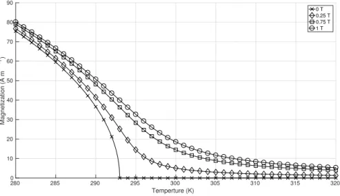
applied magnetic field in the temperature region below 280 Kelvin is negligible. However at the Curie tempera-ture and higher the magnetic dipole moments ordering will decrease. The alignment of the dipoles is very messy. Increasing the applied magnetic field will align the dipoles more.

280 285 290 295 300 305 310 315 320

Temperture (K) 0

10 20 30 40 50 60 70 80 90

Magnetization (A m

-1)

0 T 0.25 T 0.75 T 1 T

Figure 3.5.2:The internal magnetization shown at various applied magnetic field strenghts aroundTC. The

mate-rial of investigation: Gadolinium.

The effect of the hyperbolic cosine from the model is again very visible at 0T. The hyperbolic cosine behaves asymptotic at 0T and temperatures aboveTC.

The Curie temperature indicates the transition temperature: the phase transition from ferromagnetism to para-magnetism. In case of the abscence of the magnetic field the magnetization of the paramagnetic material is zero. Due to higher applied magnetic fields the transition temperature is shifted, to higher temperatures. The lines ap-pear to converge towards zero far beyond 330 Kelvin. This means that an increase in temperature will not greatly affect the magnetization, when for example the magnetic field is varied for a MCE.

3.5.3

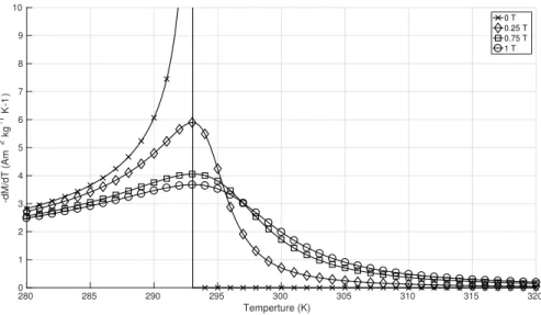
T

In the heat source equation 3.5.1, the derivative of the magnetization with respect to temperature ,³δ_δM_T´

H plays an

important role. For this reason this term is interesting to discuss and visualize aroundTC.

˙

QMCE= −Tρµ0

µδ_M

δT

¶

H

d H

d t (3.5.1)

Due to the asymptotic behaviour of the magnetization the derivative is also discontinuous, see figure 3.5.3. The amplitude of the derivative at zero field is very high. According to Kitanovsky [6] this value is expected to be much lower. The asymptotic behaviour is not a problem since the value of the derivative drops drastically when the applied magnetic field is non-zero. In figure 3.5.2 the applied magnetic field begins to affect the magnetization aroundTC. This can be seen again in the derivative. No matter how high the magnetization the derivative peaks at

280 285 290 295 300 305 310 315 320

Temperture (K)

0 1 2 3 4 5 6 7 8 9 10

-dM/dT (Am

2 kg -1 K

-1

)

0 T 0.25 T 0.75 T 1 T

Figure 3.5.3:The derivative of magnetization with respect to temperature shown at various applied magnetic field

strenghts aroundTC. The material of investigation: Gadolinium.

3.6

M

ATERIAL

P

ROPERTIES OF

M

N

F

E

P

S

I

The use of gadolinium as a MCE-material has the main disadvantage of being expensive. Next to this gadolinium is only effective in a specific temperature range which can be disadvantageous if a large temperature span is required. The effectiveness of a heat pump which relies upon the MCE with one MCM is depended on the desired tempera-ture span. During the operation of an AMR a temperatempera-ture profile is established throughout the device. Due to this temperature profile parts of the AMR are at a temperature that are, temperature wise, far away from the materials Curie temperature. The magnetocaloric effect in these parts will be much lower and decrease the performance in terms of entropy or temperature change of the AMR. In order to overcome this problem several materials with specific temperature ranges can be used in series. Several experimental and numerical studies have proven this concept [23], [24],[25].

As mentioned earlier materials that exhibit a first order behaviour in a magnetic field display latent heat. Nowa-days the preferred approach is to use this latent heat to reach large∆S and∆Tadvalues. Various material families

are known and studied that display a so-called ’giant MCE’. The materials being: Gd5(Si,Ge)4, La(Fe,Si)13and the MnFe(P,X) family with X = As, Ge or Si [12]. In this thesis the use of Mn1.25Fe0.7P1₋ySiy is being investigated as a

material for an AMR set up. The use of ’y’ indicates that several compounds can be created. In this case y = [0.49 0.50 0.51 0.52]. This compound shows remarkable magnetic and MCE properties whereas by varying the y value the transition temperature can be altered [12]. Various material properties are obtained via direct measurements as done by [12] and can be used to determine and estimate the values for other magnetic field strengths than de-termined by Yibole(2014) et. al. The dede-termined properties are later used in numerical experiments, see chapter 6.

3.6.1

H

Due to the lack of consistent heat capacity data, results of direct measurements of the magnetocaloric effect in Mn1.25Fe0.7P1−ySiy are used to obtain the heat capacity. No hysteresis is assumed for this model which can be

justified by the found limited hysteresis effect as found by Bruck [12]. This assumption leads to the justification of the irreversibility of the MCE.

determine the heat capacity, according to simple thermodynamics:

∆S=

Z 2 1 µ δq T0 ¶

i nt r ev=

1 T0

Z2

1

¡

δq¢

i nt r ev (3.6.1)

∆S₌ q T0

[J/(kg K)] (3.6.2)

In this caseT0stands for the temperature at which the entropy change has been measured. The data used is created at a magnetic field of 1 Tesla. Now the total heat per kilogram can be derived from equation 3.6.2.

Next to the entropy change the adiabatic temperature change has been measured and reported. This in turn can be used to once again determine the total heat per kilogram.

260 270 280 290 300 310 320

Temperature (K) 0 0.5 1 1.5 2 2.5 Tad (K)

Adiabatic temperature change

Mn1,25Fe0.70P0.51Si0.49 Mn1,25Fe0.70P0.50Si0.50 Mn1,25Fe0.70P0.49Si0.51 Mn1,25Fe0.70P0.48Si0.52

(a)The adiabatic temperature change at a field variation to 1

Tesla.

260 270 280 290 300 310 320

Temperature (K) 0 2 4 6 8 10 12 S (kJ/(kg K))

Entropy change at isothermal condition

Mn

1,25Fe0.70P0.51Si0.49

Mn1,25Fe0.70P0.50Si0.50

Mn

1,25Fe0.70P0.49Si0.51

Mn1,25Fe0.70P0.48Si0.52

(b)The isothermal entropy change at a field variation of 1 Tesla.

q₌cp·∆Tad i abat i c[J/(kg K)] (3.6.3)

Rewriting equation 3.6.2 and 3.6.3 provides an expression for the heat capacity:

cp=∆

S_·T0

∆Tad

(3.6.4)

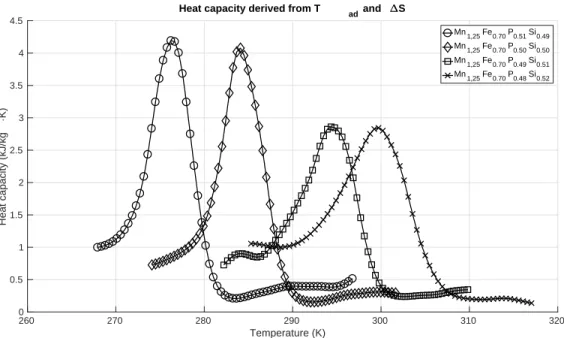
Resulting in the following figure for the heat capacity at 1 Tesla.

The first thing to notice is the immense change of heat capacity when the compounds are being held in a mag-netic field. Further to notice are the starting values, suggesting a higher heat capacity before TC and the aft TC

values, suggesting a lower heat capacity after the Currie temperature. This is also seen in gadolinium.

The maximum values in heat capacity are different from the values for the adiabatic temperature change. If a temperature profile is applied upon Mn1.25Fe0.7P1−ySiyit could be beneficial to ensure that both temperatures are

260 270 280 290 300 310 320 Temperature (K) 0 0.5 1 1.5 2 2.5 3 3.5 4 4.5

Heat capacity (kJ/kg

K)

Heat capacity derived from T _ad and S

Mn_1,25Fe_0.70P_0.51Si_0.49 Mn_1,25Fe_0.70P_0.50Si_0.50 Mn_1,25Fe_0.70P_0.49Si_0.51 Mn_1,25Fe_0.70P_0.48Si_0.52

Figure 3.6.2:The heat capacity derived from the adiabatic temperature change and isothermal entropy change at

1 Tesla.

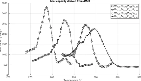
HEAT CAPACITY DETERMINATION USING d M_{d T} According to the thermodynamics of the magneto caloric effect the heat capacity can also be determined by using the magnetization data. The heat capacity change can be deter-mined using the rewritten form of equation 2.2.17. This equation provides the adiabatic temperature change due to the magnetocaloric effect. However, the latent heat is not included in this calculation.Using the magnetization data an estimate can be made of the influence of the latent heat upon the adiabatic temperature change. Which in turn provides a more accurate estimate of the heat capacity.

cp=

m_µ0 Tad ·

T· µ δM δT ¶ H· H (3.6.5)

Equation 3.6.5 requires the derivative of the magnetization with respect to temperature. Using the experimental data this derivative can be determined which in turn provides with again the heat capacity, see figure 3.6.3.

The heat capacity is now peaking at 3000_∼2500 J/kg K instead of 4200. The first method of determining the heat capacity is based upon the entropy change and temperature change. However the second method is depended on the magnetization curve. The second method does not incorporate the latent heat present during the magneti-zation, which in turn provides a lower heat capacity.

The height of the heat capacity can be justified by considering the large entropy change whilst maintaining a relative low temperature change. Even when isolating the entropy change from the heat capacity calculation provides a high heat capacity.

In essence are both method exactly the same considering the thermodynamics. The reason to calculate the heat capacity is to estimate the magnitude of the latent heat.This latent heat is also measured during the adiabatic temperature changes and is one of the reasons this material is so promising [12].

The above determined heat capacities are at 1 Tesla. For other magnetic field strengths the heat capacity is assumed as described in the following. This is done by slightly imitating the behaviour of gadolinium to incorporate the effect of the different magnetic states of the material before and after TC. At zero Tesla at temperatures before

TCa value of 900J/Kg K is assumed as heat capacity, where after TCa value of 450 J/Kg K is assumed. The same

values are assumed for temperatures away from TCat non zero magnetic field strengths.

260 270 280 290 300 310 320

Temperature (K)

0 500 1000 1500 2000 2500 3000 3500

Heat capacity J/kg K

heat capacity derived from dMdT

Mn_1,25Fe_0.70P_0.51Si_0.49

Mn_1,25Fe_0.70P_0.50Si_0.50

Mn_1,25Fe_0.70P_0.49Si_0.51

Mn_1,25Fe_0.70P_0.48Si_0.52

Figure 3.6.3: The heat capacity derived from the magnetization change and adiabatic temperature change at 1

Tesla.

Heat capacity of Mn_1.25Fe_0.7P_1-ySi_y

Temperature(K) Magnetic field strength (A/m)

0 8 1000

295 6

2000

Heat capacity J/(kg K)

290

×105 3000

4

285 4000

2 ₂₈₀

275 0

Figure 3.6.4:3D heat capacity plot for Mn1.25Fe0.7P1−ySiy. The heat capacity is interpolated between the two know

Cpcurves (H = 1T and 0T).

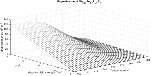
3.6.2

M

Tesla. The internal magnetization values in between zero and 1 Tesla are assumed to be on a linear interpolation field as shown in figure 3.6.5.

Magnetic field strength (A/m) Temperature(K)

0 8 20 40

284

6 ₂₈₂

60

280

Magnetization (A m

2 kg -1)

80

×105

Magnetization of Mn_1.25Fe_0.7P_1-ySi_y

4 278

100

276 120

274

2 ₂₇₂

140

270

0 268

Figure 3.6.5:3D magnetization plot for Mn1.25Fe0.7P1₋ySiy . The magnetization is interpolated between the two

know Cpcurves (H = 1T and 0T).

LATENT HEAT ANDDERIVATIVES

In order to create a heat source function that behaves more or less predictable the internal magnetic field curve is imitated with a hyperbolic tangent. Retrieving data from the literature provides no smooth curve, and therefore the derivative is not smooth either. This in turn provides a heat source function that behaves not as expected when looking at the literature. To overcome this effect imitation functions are used.

When the adiabatic temperature is calculated using these imitation functions the magnitude of the MCE is too low. This is due to the fact that the thermodynamics describe second order behaviour more accurately since no la-tent heat is involved. To accommodate for the missing lala-tent heat, the magnetization curves are slightly steepened. This in turn provides for higher derivatives and a more appropriate adiabatic temperature change. The result of this approach will be discussed in chapter 6.

3.6.3

D

Other material variables required to solve for the heat transport equations are: thermal conductivity and density. By private communication with prof. van der Meer, these values are assumed constant and in-depended of magnetic field strength or temperature. The thermal conductivity is assumed to be 44.2476_mW_·K and the density is assumed to be 5657.2kg

CHAPTER

FOUR

0D-MODEL

In the previous chapters two main subjects where introduced: the magnetocaloric effect and ways to find the material properties. This chapter will discuss the implementation of and evaluate these subjects. Previous studies at the Uni-versity of Twente have found an inconsistent energy balance, this part is devoted to investigating this inconsistency. In the end the energy balance is discussed. Following chapters will concern the description of a 2D model and the use of other materials.

4.1

M

ODEL SET UP

In order to practice the magneto caloric effect in a numerical manner the most easy way to investigate the MCE is to create an 0D model. This will provide helpful insight in the energy contributions of each part of the internal energy balance and to validate whether the energy balance is consistent. The most simple setting to use is if adiabatic conditions are applied; no heat is added or lost from external sources other than the heat source term due to the MCE. This way only equation 4.1.1 is under investigation which represents the energy balance. This equation has been derived earlier in chapter two, see equation 2.2.10. Aspects such as the geometry, the position or orientation of the applied magnetic field, hysteresis and material inconsistencies are not taken into account.

d u=ch(T,H)d T+µ0T

µ

δM

δT

¶

H+µ

0H d M (4.1.1)

4.1.1

N

I

The derived formulas for the material properties, see chapter 3, and the MCE, see chapter 2 are implemented into Matlab. Two distinctive parts can be identified: the solution script and the material property script. For this experiment gadolinium is used as the MCM.

The problem at hand is not analytically solvable and is time depended. The use of an explicit Runge-Kutta scheme is used, codename by Matlab:ode45. The system is evaluated as ’non-stiff’ which justifies the use of this scheme. However this scheme has a medium accuracy as presented by the Matlab Documentation. The main goal of this experiment is to prove the consistency of the energy balance. The consistency of the energy balance could be depending on the time-stepping of the solver algorithm. A temporal study will therefore be used at which the error in the energy balance will be studied.

In order to still gain a quantitative solution, a variation in time-steps has to be made. This variation will show to what extend the solution is depended on the time stepping and therefore the accuracy of the numerical scheme. However when the time stepping becomes small the computational time will be estimated to be very long. There-fore a relative error in the energy balance will be set at the order of 1·10−5.

The material property script will provide the values of the specific material properties such as magnetization and heat capacity. These values can be used by the solution scheme of the MCE. The solution scheme provides the conditions from which the script can calculate accurate material properties.

MATERIAL PROPERTY SCRIPT The heat capacity and the internal magnetization of gadolinium are depended on the applied magnetic field and current temperature. In order to obtain the corresponding values for these variables the script that determines these values requires the applied field and current temperature. The current temperature will be provided by the solution scheme. The mean field theory as described in chapter 3 is implemented into this script. By using both the solution and material script the solution will be calculated by using the proper material property values.

4.1.2

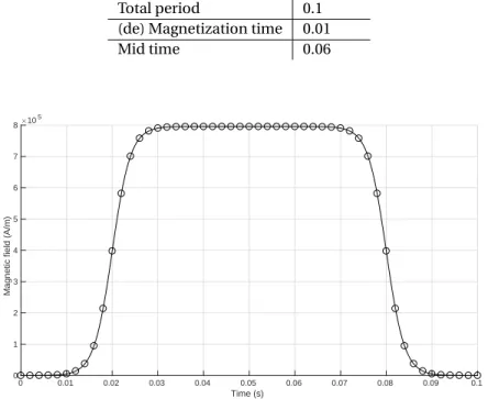
M

In order to create an numerical magnetic field a unit step function was used, see equation 4.1.2. The step function has the ability to simulate an almost instantaneously change in magnetic field strength. This is done using two step functions in series: one for magnetization and the other for demagnetization. This magnetic field will be the field where the material will respond to; geometry or material defects will not be modelled.

H(t)=1

2+ 1

2tanh(kt) (4.1.2)

Due to the nature of implementing, the step function as presented the magnetic field is not zero at the beginning and end of the simulation, therefore extra time is added before the step functions kick in. Next to this extra time is added after the magnetization step to show the adiabatic behaviour of this system. During this extra time the magnetic field strength does not change and therefore the system will come to a temporary rest at its newly acquired temperature. Since the system is adiabatic no heat losses will be implemented or expected in the result.

Table 4.1.1:Numerical applied magnetic field timings.

Parameters Value [s]

Total period 0.1

(de) Magnetization time 0.01

Mid time 0.06

0 0.01 0.02 0.03 0.04 0.05 0.06 0.07 0.08 0.09 0.1

Time (s) 0

1 2 3 4 5 6 7 8

Magnetic field (A/m)

105

Figure 4.1.1: The applied magnetic field. The field strenght varies from 0 to 1 Tesla. The value in the graph is

The derivative of the applied magnetic field is present in the heat source and therefore required in the numerical scheme. This is implemented as 4.1.3.

d H d t =k

1 2sech

2_{(kt). (4.1.3)}

The unit step functions describe only a part of the cycle. The same step is used only a delay later and multiplied by -1. This will provide a symmetrical function shape which in turn ensures cyclic behaviour in its most simple form: returning to the initial state.

0 0.01 0.02 0.03 0.04 0.05 0.06 0.07 0.08 0.09 0.1

Time (s) -1

-0.8 -0.6 -0.4 -0.2 0 0.2 0.4 0.6 0.8 1

Magnetic field (A m

-1 s -1)

108

4.2

R

ESULTS AND

D

ISCUSSION

The adiabatic temperature change realized in this model is as expected around 5.5K, see figure 4.2.1. The tempera-ture remains at a constant value which implicates no heat loss. After de-magnetization the temperatempera-ture reaches its original temperature. This indicates that the model accurately reacts upon the applied magnetic field and its other boundary conditions. This figure has been acquired at low time-stepping.

0 0.01 0.02 0.03 0.04 0.05 0.06 0.07 0.08 0.09 0.1

Time (s) 290 291 292 293 294 295 296 297 Temperature (K)

Figure 4.2.1:The adiabatic temperature change plotted againts time. The model was set aroundTC. This condition

makes for a clear change in temperature on macro scale.

Every term of the the energy balance as presented in equation 2.3.6, repeated at equation 4.2.1, can be deter-mined separately and are shown in figure 4.2.2. The heat source term experiences the highest energy difference. The temperature change is the largest contributor for the internal energy to raise. The magnetic work energy how-ever is negative. In order to magnetize the material, energy is taken up by the material.

0 0.01 0.02 0.03 0.04 0.05 0.06 0.07 0.08 0.09 0.1

Time (s) -200 0 200 400 600 800 1000 1200 1400 1600

Energy (J kg

-1)

Total generated Heat Internal Energy Magnetic Work

Figure 4.2.2:The energies plotted over time. Every line represents a term of the energy balance.

∆u(t)₌

ZT(t)

Ti

cH(T,H)d T+

Z H(t)

0 T_µ0

µ

δM

δT

¶

H

d H₋

Z H(t)

0 µ0

In order to prove that the thermodynamics are consist of the MCE the internal energy balance was evaluated at a small time-step. Every part of the energy balance can be calculated and plotted versus time. See figure, 4.2.2.

error[₋]₌

 

RT(t)

Ti cH(T,H)d T

³ RH(t)

0 tµ0

³

δM

δT

´

Hd H

´

+³RH(t)

0 µ0Md H

´ 

 (4.2.2)

Equation 4.2.2 can be plotted, see figure 4.2.3. The relative error has not the same value throughout the entire period. This is due to numerical effects; at the the times the slope of the error is higher than 0, the (de)magnetization kicks in. The relative error is evaluated at half the total period, t = 0.05s. Thed H_{d t} is zero here and there is no change in state. The value of the error is 3.82_·10−5_{at this time.}

0.035 0.04 0.045 0.05 0.055 0.06 0.065

time(s) 3.805 3.81 3.815 3.82 3.825 3.83 3.835 3.84 Relative Error(-) 10-5

Figure 4.2.3:The error with respect to the internal energy plotted against time.

4.2.1

T

S

The magneto caloric effect is a time depended phenomena and can be calculated using various time-steps in the numerical solution scheme. The accuracy of the solution and therefore the energy balance seems to be depended on the time-stepping. Various time-steps have been used to calculate the energy-balance-error and are shown in table 4.2.1. The error seems to decrease towards engineering and scientific standards as the time step also de-creases. This justifies the statement of the time-dependency of the MCE and the accuracy being depended on the time step.

Table 4.2.1:The error as calculated in equation 4.2.2, displayed against the time-stepping.

Time Step (s) Error(-)

0.01 0.99

0.005 0.89

1_·10−3 _4.40

·10−3 5_·10−4 _3.75

·10−4 1_·10−4 _1.88

4.2.2

D

As can be seen in the previous section the energy balance error is below the engineering standard of 1·10−3and somewhat above the scientific standard of error of 1·10−6. In this study it was found that the error decreases with smaller time steps. Therefore it is assumed that the energy balance is consistent only that the solution is depended on the time step. This in turns justifies the assumption that the thermodynamics are consistent as well. The accuracy of the solution seems to be depended on the time step size used in the solver.

However previous work at the University of Twente shows an in consistency in the energy balance [26] and [27]. Looking at the magnitude of their error it seems that the magnetic work has not been taken into account. When not taking the magnetic work into account at the error calculation the magnitude of this error resembles the error found in previous work.

CHAPTER

FIVE

ACTIVE MAGNETIC REGENERATOR

The previous chapter discussed the mechanism of the MCE and proved its energy balance. The current chapter will discuss the graded AMR, the numerical set-up and several parameters in general. The numerical set-up will be vali-dated using literature.

5.1

2D

MODEL

- G

ADOLINIUM

As discussed the AMR provides for a higher efficiency in terms of heat transport than a cascade system or otherwise [18], [28].

For an experimental set-up it is desirable to have proper dimensions which could lead to experimental results that have considerate meaning. Obtaining these dimensions could be done via a numerical study. The main goal of this study is to provide such dimensions. This part of the thesis consists out of two parts: the first parts discusses and studies the effect of the temporal and spatial resolution in a numerical scheme and the second part one im-portant variable: the utilization factor. This factor will be explained later. This factor plays an imim-portant role in designing a experimental set-up consisting out of the Mn1.25Fe0.7P1₋ySiy material family. The first part consists

out of a model of an AMR modelled in Comsol. The material used in this model is gadolinium. The reason for this material is that various studies both numerically and experimentally have been conducted and using the out-come of those studies can provide insight in the performance of the numerical set-up. Performing a temporal and spatial study provides helpful insight in to the accuracy of the outcome with respect to the previous studies versus computational time.

The second part investigates the behaviour of Mn1.25Fe0.7P1−ySiyin an AMR setting. For this study one variables

are studied resulting in an recommendation for an experimental set-up. Most of the dimensions are determined by an study performed by Paolo et. al. [29].

The AMR contains a porous structure of a magnetocaloric material. Through this porous structure a heat-transfer fluid is pumped with an oscillatory velocity pattern depending on the magnetization state. The AMR has two functions in a magnetic refrigerator: it works as the heat regenerator as the refrigerant. In general 4 steps of the AMR operation can be identified. These steps are in general analogue to the vapour-compression refrigerator cycle. These steps are:

• MagnetizationThe domain is exposed to an external magnetic field. Therefore the magnetization deriva-tive becomes posideriva-tive and the magnetocaloric effect occurs. This leads to an temperature increase due to adiabatic conditions. See figure 5.1.1a.

• Fluid flowNow the MCM is heated up it can be cooled by letting a fluid flow from the cold side, or cold-heat exchanger, to the hot side removing the cold-heat from the MCM. The removed cold-heat is either transported to another part of the MCM or dumped at the hot-heat exchanger. See figure 5.1.1b.

• Fluid flowalso called hot-blow: fluid is moved from the hot heat exchanger trough the AMR. This fluid is cooled by the AMR and eventually dumped into the cold heat exchanger. This last step removes heat from the cold side. Now the cycle is complete. See figure 5.1.1d.

(a)The magnetization step in the AMR-cycle (b)Fluid movement from the Cold-heat exchanger trough the

AMR: second part of the AMR-cycle

(c)Removing the magnetic field, leading to a decrease in

tem-perature: third part of the AMR-cycle.

(d)Fluid movement from the hot-heat exchanger trough the

AMR: last part of AMR cycle

Figure 5.1.1:Figure used from [30]

The AMR-cycle can be described via an T-S diagram as showed in figure 5.1.2. This figure describes the AMR cycle at a given point in the regenerator. The entropy is considered as the total entropy of a given point including both the solid and the fluid.

The cycle starts with the magnetization as displayed in figure 5.1.1a. First the MCM is adiabatically exposed to a magnetization step. The fluid movements are displayed from B to C and D to A, which are displayed in figure 5.1.1b and 5.1.1d. Where the entropy is changing, however the temperature alters very little. The demagnetization step is removed in process C to D and is done adiabatically, which also is displayed in figure 5.1.1c.

Figure 5.1.2:Every indiviudal process of the AMR cycle. The schematic in this figure represents the T-S-diagram of each process for an infinitesimal part of the regenerator [18].

5.2

M

ODEL

D

ESIGN

For the validation the theoretical cooling capacity and maximum temperature span of an AMR device using gadolin-ium are under investigation. Previous work of master students has delivered a 2-D model of an AMR device based on a regenerator with parallel plates of gadolinium modelled via the mean field theory [27].

The main goal of this part of the study is to investigate a proper spatial and temporal resolution. Various other work has been done on a parallel plate AMR containing gadolinium, [18], [8],[17], [9]. These provide parameter studies both in numerical and experimental set-ups.

The domain consists out of a simplified parallel plate AMR-set up, see figure 5.2.1. It is a two-dimensional model and simulates half a replicating cell. The cell consists out of half a plate of MCM and half a fluid channel. The x-direction is parallel to the plates, which also is indicative for the fluid flow. The y-direction is perpendicular to the plates. The z-direction is not represented by the model, hence its 2D-character: the cell is assumed to have an infinite width.

Solid Fluid

Length MCM (mm)

Thickness MCM (mm)

Thickness Fluid (mm) Length Fluid (mm)

Insulation C- or H-HEX

Symmetry

Symmetry

x y

Figure 5.2.1:Numerical 2D domain, representing the AMR.

The approximation can be assumed sufficient for the flow but could be insufficient in terms of the thermal coupling to the ambient via boundary conditions. Heat losses are not assumed in this original model.

δTf

δt =

kf

ρfcf

Ã

δ2_T

f

δx2 +

δ2_T

f

δy2

!

−(u· 5)Tf (5.2.1)

δTs

δt =

ks

ρscs

µδ2_T

s

δx2 +

δ2_T

s

δy2

¶

(5.2.2)

The subscripts denote the solid and fluid by s and f. The fluid equation, 5.2.1, consists out of two terms: the diffusion term and convective term. The velocity field is denoted by, u, is obtained by solving the Navier-Stokes equation for the flow problem. In this problem the assumption is made that the plates are infinitely wide and are very close to each other. For the solid equation, 5.2.2, the transient term and diffusive term are applied. The thermal conductivity is denoted by k, the density byρand the specific heat by c. All thermal and material properties are assumed constant except for the heat transfer, see chapter 3.

In order to properly assume adiabatic magnetization the magnetization will be done instantaneously. This way equation 2.2.17 can be used. The MCE will be formulated as a source term, which gives the following:

δTs

δt =

ks

ρscs

µδ2_T

s

δx2 +

δ2_T

s

δy2

¶

+QMCE (5.2.3)

Where QMCEis derived in chapter 2 and repeated here:

Q_{MCE= −}TρcH

µδ_M

δT

¶

H

d H

d t (5.2.4)

The hot heat exchanger is provided with a set temperature, independent from the systems performance. Other boundaries include thermal insulation and symmetry.

5.2.1

T

T

The energy equation, 5.2.1, contains the convective term,₋(u₅)Tf, in which the fluid velocity is represented. This

fluid flow is discretized by using the following analytical expression for the velocity field[8]:

u(y)=u˜

Ã

6y2 H2_f −1/2

!

(5.2.5)

This expression holds for steady, laminar fluid motion between to infinitely wide parallel plates. ˜uis the mean fluid velocity andHf the height of the fluid channel.

5.2.2

I

In this subsection various parameters will be discussed and defined for further usage in later chapters.

TIMINGS

As described in the previous section four stages of the magneto refrigeration cycle can be identified. Every stages has a duration time ofτxwhere x = 1,2,3,4. τ1andτ3represent the (de)magnetization timing and have the same value. τ2andτ4represent the fluid flow timings. The fluid flow timings will also be identical to each other. This creates a symmetrical timing pattern. However, this symmetrical timing pattern for the fluid flow could be favoured due to the changing heat capacity during (de)magnetization. Such asymmetrical timing is more difficult to imagine since it could induce an imbalance in the flow system: a net mass transport in positive or negative x-direction. However the asymmetrical timing is not considered further and of interest for future work.

GEOMETRIC PARAMETERS

The regenerator can be geometrically defined using three variables:Lslength of the regenerator,Hsthe thickness

of the solid part and the thickness of the fluid channel,Hf. Now the porosity of the regenerator can be defined:

²=¡ Hf

Hf +Hs

¢ (5.2.6)

In order to determine the pressure drop across the regenerator the hydraulic diameter is required: defined as four times the flow cross section, divided by the wetted perimeter:

DH=2Hf (5.2.7)

FLOW PARAMETERS

Duringτ2andτ4the flow is characterized by equation 5.2.5, the fluid inlet velocity, which is an input parame-ter. The fluid flow is modelled by two step functions, where the magnitude is determined by ˜u. The second step function is in the opposite direction, creating a oscillatory flow.

Next to this the flow is characterized by the properties of the heat transfer fluid. The following relation is used to determine the length of a blow, or how far a fluid element is moved by average:

δx₌u˜τ2 (5.2.8)

For now it is relevant to consider the utilization factor,ϕ. This dimensionless parameter can be used to compare experimental results with numerical and is defined as the ration between the total thermal mass of the fluid moved and the thermal mass of the regenerator material:

ϕ=m˙_mfcfτ2

scs

(5.2.9)

In case of a parallel plate situation this can be rewritten to:

ϕ=ρfcfHfδx

ρscsHsLs

(5.2.10) (5.2.11) The expression, 5.2.10, contains the heat capacity for the solid in the denominator. As discussed in chapter 3, this variable is strongly depended on temperature and magnetic field strength. As described in [31], the heat capacity used for a single material AMR is taken at TCand 0T external magnetic field. When considering multiple

materials a different approach is used: a weighted average would be more appropriate. The utilization factor and

τ2are thus used to determine the ˜u.

5.2.3

M

T

Due to the high non-linear behaviour of the magneto caloric effect numerical studies are justified. This in turn leads to the question what are the proper discretization dimensions. In order to obtain a reasonable temporal and spatial discretization an analytic attempt will be made in terms of the cooling capacity. In this case the regenerator will be simplified to have a single heat capacity and constant, albeit artificial, adiabatic temperature change. Assumed is a steady state condition and in this condition the magnetic work under no-load conditions should be equal to the amount of heat leaving the hot-side of the regenerator. The expression used for this condition is:

wmag=csρs(∆Tad,mag+∆Tad,d emag)LsHs (5.2.12)

In equation 5.2.12 Lsand Hsrepresent the dimensions: length and height of the regenerator. Ifcsis chosen 235

Jkg−1_K−1_{, which is a value representing the main heat capacity around the Curie temperature and letting∆T}

admag=