3D Recognition Using Affine Invariants
Ahmed El Oirrak, Mustapha Elhachloufi, Elmustapha Ait Lmaati, Mohamed Sadgal, Mohammed Najib Kaddioui
Faculty of Science Semlalia, LISI Laboratory, Marrakech, Morocco. Email: [email protected]
Received January 22nd,2011; revised October 28th, 2011; accepted January 5th, 2012
ABSTRACT
The size of 3D data stored around the web has become bigger. Therefore the development of recognition applications and retrieval systems of 3D models is important. This paper deals with invariants for 3D models recognition. Thus un- der general affine transform we propose in a first time determinants of three points to realize invariance under affinity. To solve starting point problem we needs Fourier Series (FS) to extract affine invariant descriptors, called Fourier Se- ries Descriptor (FSD). The difference between first and second approaches: in first approach determinants are computed on cartesian coordinates directly while in the second one determinants are computed from FS coefficients to eliminate dependency on starting point. The FS are also applied on 2D slices to generate affine invariants for 3D volume. FS can be computed based on hole points of volume, but this technique. The principal advantages of proposed ap- proaches are the possibility to handle affine transform and 3D volume. Two types of 3D objects are used in the ex- perimentations: mesh and volume, the Princeton Shape Benchmarek (PSB) is also used to test our descriptor based on FSD.
Keywords: Affine Invariant; FSD; Mesh; Volume; 2D Slice
1. Introduction
The digital databases of 3D objects which are used in various domains (e-commerce, games, medicine, etc.) become large. Therefore, an efficient method that allows users to find similar 3D objects for a given 3D model query is becoming necessary. Content based indexing and retrieval is an important way to manage these data- bases. Many content based retrieval systems and search engines for 3D models are available on the web [1-3]. Many methods in this way are developed. The shape spectrum descriptor proposed by Zaharia et al. based on surface geometry, is recommended by MPEG-7 [4]. Fi- lali et al. proposed the descriptor based on 2D views named Adaptive Views Clustering (AVC). It is a proba- bilistic Bayesian method that selects the most interesting views from several views of a 3D model [1]. Based on the statistics, Osada et al. proposed the descriptor named shape distribution (D2) [5]. Paquet et al. proposed the method of cord histograms [6]. The ratio area/volume is used as a feature vector to describe the 3D models by Zhang and Chen [7]. Even if this descriptor computes the feature vectors easily and quickly, it needs a high quality of mesh. Vranic and Saupe [8] proposed the method named Ray based descriptor. It uses the extents obtained from the center of mass of the model to intersection with its surface in directions which are constructed by an ico-
sahedron. This approach is not robust to noise and needs a high dimension of feature vectors, this is why the authors construct the feature vectors from the complex function on a sphere, composed with Ray based feature vectors and shading based feature vectors, presented in frequency domain by applying the spherical harmonics [9]. In order to capture the information in the interior of a 3D model, the authors proposed the descriptor named Layered Depth Spheres [10], where they use the property of spherical harmonics to achieve the rotation invariance. All previous work cited above can handle only 3D similitude (rotation, scale, translation).
The principal advantages of proposed approaches is the possibility to handle affine transform and 3D volume. Two types of 3D objects are used in the experimentations: mesh and volume, the Princeton Shape Benchmarek (PSB) is also used to test our descriptor based on FSD.
The paper is organized as follow: in Section 2, deter- minants of three points are introduced as affine invariants for 3D mesh. However to solve the starting point problem we apply Fourier series on separates coordinates to obtain what we call FSD in Section 3. In Section 4 FSs coefficients are derived from 2D slices to generate affine invariants for 3D volume. PSB database is used in Section 5 as a direct application of FSD method on 3D mesh. Section 6 presents some mathematical and experimental comparisons.
2. Invariants under 3D Affinity Using
Determinant of Three Points
A general affine transform A Equation (1) is defined by the following matrix:
11 12 13
21 22 23
31 32 33
a a a
a a a
a a a
A (1)
Let X be a set of 3D points, then the analytic ex- pression Equation (2) of the transformed set X is given by:
11 12 13
21 22 23
31 32 33
i i i
i i i
i i i
i i i
x a x a y a z
y a x a y a z
z a x a y a z
(2)
The determinant of three points Equation (3) is given by:
det
i j k
i j k
ijk
i j k
x x x
y y y
z z z
D (3)
For each three points we can verify that: det( )
ijk ijk
D A D (4)
The resulting (3 × 3) matrix Dijk depends on choice
of index i, j and k for X and X.
3. Starting Point Problem and FSD Method
The starting point problem can be seen as dependency on index of points, the following example of a 2D curve illustrates this problem: a circle can be generated by:
x t y t( ), ( )
cos ( ),sin( )t t t
where t
0; 2π
.Therefore the following equation:
x tt0 ,y tt0
cos
tt0
,sin
tt0
where t
0; 2π
and 0 a constant can give a circlebut the order of points are not the same. t
In many shape descriptors, the curve is re-parame- terized by normalized arc length Equation (5), s which is defined as follows:
( )s t
x y z
(5) Arc length is preserved under similarity transforms i.e. the corresponding points between the original and the transformed curve have the same normalized arc length under change in orientation, translation, and differ by a scale factor under scaling. Arc length is not preserved under general affine transforms [11]. In some applications, where curves are subject to general affine transforms, arc length is replaced by affine length Equation (6) which is defined as follows and is proved to be affine invariant.
( )t x yz zy y xz zx z xy yx
(6) The analytic expression of the transformed and repara- meterized set X Equation (7) is:11 12 13
21 22 23
31 32 33
( ) ( ) ( ) ( )
( ) ( ) ( ) ( )
( ) ( ) ( ) ( )
x a x a y a z
y a x a y a z
z a x a y a z
(7)
To extract invariant we develop separately x, y and z into FSs as following:
=( ) 2π =
=
( ) 2π =
=
( ) 2π = FS FS FS n x jn n n n y jn n n n z jn n n c e x c e y c e z
(8) where 2( ) 2π
2 2
( ) 2π
2 2
( ) 2π
2
1 ( ) d
1 ( ) d
1
( ) d
T x j n T T y n T T z j n T
c x e
T
c y e
T
c z e
T n j n n
(9)T denote the period of parameter .
2
( ) 2π
2
2 2π
11 12 13
2
2 2π
11 2
2 2π
12 2
2 2π
13 2
( ) ( ) ( )
11 12 13
1
= ( ) d
1
= ( ) ( ) ( )
1
= ( ) d
1
( ) d
1
( ) d
=
T
x j n
n T
T j n
T
T j n
T
T j n
T
T j n
T
x y z
n n n
c x e
T
a x a y a z e
T
a x e
T
a y e
T
a z e
T
a c a c a c
d
Thus ( ) ( ) ( ) ( )11 12 13
( ) ( ) ( ) ( )
21 22 23
( ) ( ) ( ) ( )
31 32 33
x x y
n n n
z n
y x y
n n n
z n
z x y
n n n
c a c a c a c
c a c a c a c
c a c a c a c
z n (10)
We can construct relative invariant, based on deter- minant of three FS coefficients (indexed m, n and p) as follow:
( ) ( ) ( ) ( ) ( ) ( ) ( ) ( ) ( )
x y z
m m m
x y z
mnp n n n
x y z
p p p
c c c
C c c c
c c c
(11)
Thus absolute invariant (FSD) can be derived by dividing by another relative invariant , ( , and are three fixed coefficients). m n p0 0 0
C m0 n0
0 p
0 0 0
mnp mnp
m n p
C I
C
(12)
4. Affine Invariants for 3D Volume Using FS
Applied on 2D Slice
Typical scalar volume data is composed of a 3-D array of data and three coordinate arrays of the same dimensions. The coordinate arrays specify the x-, y-, and z- coordinates for each data point. The units of the coordinates depend on the type of data. For example, flow data might have coordinate units of inches and data units of psi. Slice planes provide a way to explore the distribution of data values within the volume by mapping values to colors. You can orient slice planes at arbitrary angles, as well as use nonplanar slices. In this case each volume V is characterized by a set of slices, each slice is a 2D image having coordinates (x, y) and color information.
To extract affine invariants we apply FS on coordi- nates x and y using color as parameter [12,13]. From our image we first define the set of parameterized points:
3
3
3
, , ,
, ( ), ( )
, ,
R x y G x y B x y
x y
R x y G x y B x,
y (13)
Then, we develop separately x and y into FS Equation (14) as following:
=
( ) 2π
=
=
( ) 2π
= FS ( ) =
FS ( ) =
n x jn n n n y jn n n c e x c e y
(14)We can construct relative invariant Equation (15), based on two FS coefficients (indexed m and n) as follow:
( ) ( ) ( ) ( )
x y
m m
mn x y
n n
c c
C
c c
(15)
Absolute invariant (FSD) can be derived by :
0 0 mn mn m n C I C
(16)
In Figures 2 and 3 we present five slices of a 3D volume and it’s transformed, those volumes Figure 1 are initially stocked into 24 slices.
[image:3.595.68.279.81.344.2]In this experiment only slices 1, 8 and 27 are considered. For each one six normalized color coefficients are extracted. In Table 1 invariant color coefficients are presented for original slices 1, 8 and 27. In Table 2 in- variant color coefficients are presented for transformed slices 1, 8 and 27. The result obtained allow to detect
[image:3.595.315.529.454.567.2]Figure 1. A 3D volume and its transformed. (a) MRI vo- lume; (b) Transformed volume.
Figure 2. Five 2D slices of 3D volume.
[image:3.595.309.537.600.721.2]Table 1. Six invariant coefficients for each slice of V.
slice 1 slice 8 slice 27
[image:4.595.58.286.100.202.2]2.1298 3.5516 1.3817 0.3842 0.1887 0.2907 0.2912 0.3892 0.2188 0.4825 0.5262 0.6793 0.3140 0.3626 0.5440 0.4386 0.4805 0.5930
Table 2. Six invariant coefficients for each slice of V .
slice 1 slice 8 slice 27
2.1252 3.5407 1.3851 0.3845 0.1880 0.2927 0.2892 0.3924 0.2173 0.4832 0.5315 0.6810 0.3139 0.3642 0.5477 0.4392 0.4768 0.5940
similarity between slices and consequently between 3D volume.
[image:4.595.312.533.228.379.2] [image:4.595.57.286.232.332.2] [image:4.595.311.534.411.621.2]This technique suppose that V and are stocked with the same number of slices. We can use another technique based on isosurface [14]. An isosurafce define the 3D volume bounded by a particular isovalue. The volume inside contains values greater (or less) than the isovalue. The volume outside contains values less (or greater) than the isovalue. The isovalue can be an in- terval [min, max] in this case the isosurface is a list of all cells for which the isovalue is contained in the interval [min, max]. Also the choice of isovalue on V and is another problem. Figure 4 shows some subvolumes obtained by this technique.
V
V
5. 3D Search Engine for 3D Mesh
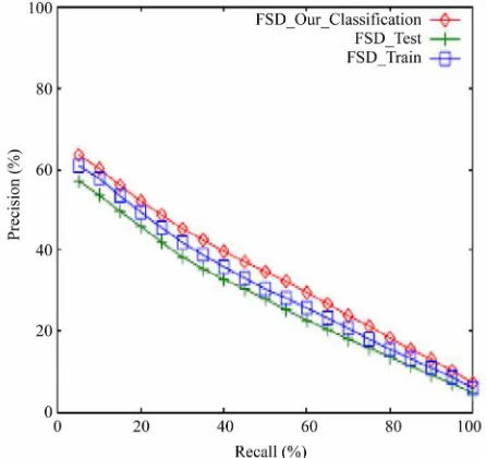
In order to test our 3D descriptor Figure 5, we use the Princeton Shape Benchmark database (PSB) [15]. It consists of 1814 3D models given in format Object File Format (OFF), with two sets (test set and train set) of classified 3D models. The test classification consists of 907 models classified into 92 classes. The training classi- fication consists of 907 models classified into 90 classes. We add some 3D models to the PSB database, which have been created using QSlim software [16] so as to provide models with different levels of detail. The modified PSB consists of 1889 models reclassified with geometrical aspects, our classification consists of 982 models classified into 93 classes. We use the average precision versus recall plots Figure 6 and the First Tier (FT), Second Tier (ST), and Nearest Neighbor (NN) quantities widely used in shape retrieval community to
Figure 4. Subvolumes obtained by isosurface technique.
Figure 5. Screen-shot of the 3D search engine.
Figure 6. Precision/recall plots for our classification, test classification and train classification using PSB database.
following formulas:
Recall = Rk N 1 Precision Rk K
The First Tier is the same as precision value when K is equal to n – 1, the Second Tier is also the same as precision value when K is equal to 2(n – 1) and the Nearest Neighbor measure is the percentage of the closest matches that belong to the same class as the query. Obviously, an ideal score is 100, and higher scores represent better results.
Figure 6 shows the recall versus precision of test set, the training set and PSB Database. After training and testing the precision becomes higher using the hole database which mean a considerable amelioration and best performance of FSD method.
6. Comparison
6.1. Mathematical Comparison
Feature vectors for 3D model retrieval can be based also on 3D moments. In [17] a complete set of orthogonal 3D Zernike polynomials is proposed based on 3D moments. Let
x y z, ,
be a local continuous density function, for example, this can be 1 inside voxels belonging to an object and 0 in free space. Traditional 3D moments pqrare defined Equation (17) as:
, ,
d d dp q r
pqr x y z x y z x y z
(17) But those moments can not handle affine transform, so we propose separable 1D moment Equation (18).
( ) ( )
( ) ( )
( ) ( )
d
d
d
x n
n
y n
n
z n
n
m x
m y
m z
(18)
We can verify as we have done in Section 3 that those moments are affine invariants.
6.2. Experimental Comparison
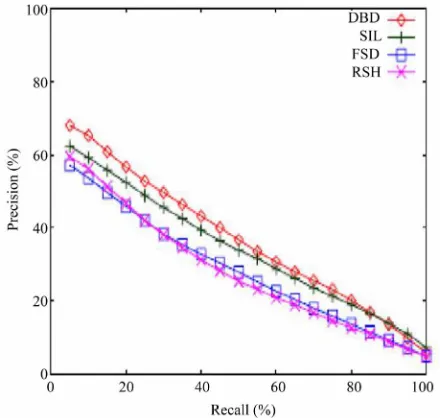
We compare our approach to the descriptor named Ray with spherical harmonic (RSH), proposed by Vranic and Saupe [21]. In order to extract the feature vector for a 3D model the authors use the continuous principal compo- nent analysis to align the model into the canonical position. Then they extract the maximal extents from the center of mass of the model to its surface, finally the spherical harmonic is applied to represent these rays in the frequency domain. The second descriptor used in comparison is the Silhouette based feature vectors (SIL), proposed by Heczko et al. [18]. This approach aligns
[image:5.595.313.533.372.581.2]models using the CPCA (Continuous Principle Compo- nent Analysis), capture shape characteristics of models in three monochromes images. Then the authors extract the three contours and for each contours they apply the dis- crete Fourier Transform in order to present feature vectors in spectral domain. The third descriptor used in the comparison is the descriptor named Depth Buffer (DBD), it is an efficient image-based descriptor proposed by Heczko et al. [18]. It needs the CPCA to align the model in a canonical position and scale into the canonical unit cube. Six grey-scale images are rendered using parallel projection. Then the authors apply 2D Fourier Transform, and their feature vectors are composed in the low frequency coefficients. Figure 7 shows the average precision versus recall plots comparing the four descriptors, where the dimension of the DBD, SIL, FSD and RSH are 438, 300, 300 and 136 respectively. Table 3 provides comparative performance measures of the different descriptors (DBD, SIL, FSD and RSH). It is clear from Table 3 that the proposed approach gives lower per- formance than DBD and SIL. However, it is worth mentioning that DBD and SIL methods are 2D view based approaches.
[image:5.595.307.540.647.733.2]Figure 7. Precision/recall plots comparing FSD method to RSH, SIL and DBD using PSB database.
Table 3. Comparison of measurements: NN, FT and ST for different methods using PSB database.
ST (%) FT (%) NN (%)
DBD 44.7 34.2 61.3
SIL 43.6 32.6 55.7
FSD 38.9 28.4 52.3
7. Conclusion
This paper advocate the use of affine invariants to describe 3D objects. Those 3D descriptors are based on determinants and Fourier series. The principal advantages of our description is that similarity is achieved without aligning models orientation by CPCA (Continuous Prin- cipal Component Analysis) and a general affine transform is considered. CPCA can gives erroneous alignments for example aircrafts with long and small wings can be aligned in tow different canonical positions. In future the 3D search engine can be extended for medical databases (MRI magnetic resonance imaging), this data typically contains a number of slice planes taken through a volume, such as the human body. One of the key difficulty when using proposed invariants is the lack of clear interpre- tation of the invariant’s meaning relatively to the shape. It may interesting to study the behavior of these invari- ants for families of synthetic shapes controlled by only a few parameters.
REFERENCES
[1] T. F. Ansary, M. Daoudi and J. P. Vandeborre, “A Bayes- ian 3D Search Engine Using Adaptive Views Clustering,” IEEE Transaction on Multimedia, Vol. 9, 2007, pp. 78- 88. doi:10.1109/TMM.2006.886359
[2] E. A. Lmaati, A. El Oirrak and M. N. Kaddioui, “3D Model Retrieval Based on 3D Discrete Cosine Trans- form,” International Arab Journal of Information Tech- nology, Vol. 7, No. 3, 2010, pp. 264-271.
[3] E. A. Lmaati, A. El Oirrak and M. N. Kaddioui, “A 3D Search Engine Based on 3d Curve Analysis,” Signal, Im- age and Video Processing, Vol. 4, No. 1, 2009, pp. 89-98. [4] MPEG-7 Video Group, “Information Technology Multi-
media Content Description Interface,” Part 3: Visual, ISO/ IEC FCD, 15938:3/N4062, MPEG-7, 2001.
[5] R. Osada, T. Funkhouser, B. Chazelle and D. Dobkin, “Matching 3D Models with Shape Distributions,” Pro- ceedings of the International Conference on Shape Mod- eling & Applications, Genova, 2001, pp. 154-166. [6] E. Paquet and M. Rioux, “A Query by Content Software
for Three-Dimensional Models Databases Management,” Conference on Recent Advances 3-D Digital Imaging and Modeling, Ottawa, 12-15 May 1999, pp. 345-352.
[7] D. Y. Chen, M. Ouhyoung, X. P. Tian and Y. T. Shen, “On Visual Similarity Based 3D Model Retrieval,” Euro-graphics, Vol. 22, No. 3, 2003, pp. 223-232.
[8] D. V. Vranic and D. Saupe, “3D Model Retrieval with Spherical Harmonics and Moments,” B. Radig and S. Florczyk, Eds., Proceedings of the 23rd DAGM-Sympo- sium on Pattern Recognition, Munich, 2001, pp. 392-397. [9] D. V. Vranic and D. Saupe, “Description of 3D Shape
Using a Complex Function on the Sphere,” IEEE Interna- tional Conference on Multimedia ICME, Vol. 1, 2002, pp. 177-180.
[10] D. V. Vranic, “An Improvement of Rotation Invariant 3D-Shape Descriptor Based on Functions on Concentric Spheres,” IEEE International Conference on Image Proc- essing, 14-17 September 2003, pp. 757-760.
[11] J.-L. Dugelay, A. Baskurt and M. Daoudi, “3D Object Processing: Indexing Compression and Watermarking,” John Wiley Sons Inc., New York, 2008.
[12] A. Eloirrak, M. Daoudi and D. Aboutajdine, “Affine In- variant Descriptors Using Fourier Series,” Pattern Rec- ognition Letters, Vol. 23, No. 10, 2002, pp. 1109-1118. doi:10.1016/S0167-8655(02)00027-2
[13] A. Eloirrak, M. Daoudi and D. Aboutajdine, “Affine In-variant Descriptors for Color Images Using Fourier Se- ries,” Pattern Recognition Letters, Vol. 24, No. 9, 2003, pp. 1339-1348.doi:10.1016/S0167-8655(02)00375-6 [14] Udeepta, D. Bordoloi and H.-W. Shen, “Space Efficient
Fast Isosurface Extension for Large Datasets,” IEEE Visu- alization, Washington DC, 19-24 October 2003, pp. 201- 208.
[15] P. Shilane, M. Kazhdan, P. Min and T. Funkhouser, “The Princeton Shape Benchmark,” Shape Modeling Interna-tional, 2004, pp. 345-352.
[16] M. Garland and P. Heckbert, “Surface Simplification Using Quadric Error Metrics,” Proceedings of the 24th Annual Conference on Computer Graphics and Interactive Tech- niques, 3-8 August 1997.
[17] M. Novotni and R. Klein, “3D Zernike Descriptors for Content Based Shape Retrieval,” Proceedings of the Eighth ACM Symposium on Solid Modeling and Applications, Seattle, 16-20 June 2003, pp. 216-225.
doi:10.1145/781606.781639