Application, Evaluation, and Process Analysis of the US EPA’s 2002 Multiple Pollutant Air Quality Modeling Platform

Application, Evaluation, and Process Analysis of the US

EPA’s 2002 Multiple-Pollutant Air Quality

Modeling Platform

Kai Wang, Yang Zhang*

Department of Marine, Earth, and Atmospheric Sciences, North Carolina State University, Raleigh, USA

Email: *[email protected]

Received May 7, 2012; revised June 1, 2012; accepted June9, 2012

ABSTRACT

A multiple-pollutant version of CMAQ v4.6 (i.e., CMAQ-MP) has been applied by the US EPA over continental US in 2002 to demonstrate the model’s capability in reproducing the long-term trends of ambient criteria and hazardous air pollutants (CAPs and HAPs, respectively) in support of regulatory analysis for air quality management. In this study, a comprehensive model performance evaluation for the full year of 2002 is performed for the first time for CMAQ-MP using the surface networks and satellite measurements. CMAQ-MP shows a comparable and improved performance for most CAPs species as compared to an older version of CMAQ that did not treat HAPs and used older versions of na- tional emission inventories. CMAQ-MP generally gives better performance for CAPs than for HAPs. Max 8-h ozone (O3) mixing ratios are well reproduced in the O3 season. The seasonal-mean performance is fairly good for fine particu-

late matter (PM2.5), sulfate , and mercury (Hg) wet deposition and worse for other CAPs and HAPs species.

The reasons for the model biases may be attributed to uncertainties in emissions for some species (e.g., ammonia (NH3),

elemental carbon (EC), primary organic aerosol (POA), HAPs), gas/aerosol chemistry treatments (e.g., secondary or- ganic aerosol formation, meteorology (e.g., overestimate in summer precipitation), measurements (e.g.,





SO 

3

NO), and the use of a coarse grid resolution. CMAQ cannot well reproduce spatial and seasonal variations of column variables except for nitrogen dioxide (NO2) and the ratio of column mass of HCHO/NO2. Possible reasons include inaccurate seasonal

allocation or underestimation of emissions, inaccurate BCONs at higher altitudes, lack of model treatments such as mineral dust or plume-in-grid process, and limitations and errors in satellite data retrievals. The process analysis results show that in addition to transport, gas chemistry or aerosol/emissions play the most important roles for O3 or PM2.5,

respectively. For most HAPs, emissions are important sources and cloud processes are a major sink. Simulated

2 2 3

H O HNO

P P and HCHO/NO2 indicate VOC-limited chemistry in major urban areas throughout the year and in other

non-urban areas in winter, but NOX-limited chemistry in most areas in summer.

Keywords: Multi-Pollutant; Air Toxics; Model Evaluation; Process Analysis

1. Introduction

Hazardous air pollutants (HAPs) or air toxics are the pol- lutants known to cause serious effects on human health, such as cardiovascular, neurological, and other organ system problems and adverse environmental issues. 188 air toxics are identified and regulated under the 1990 Clean Air Act. HAPs are emitted from a variety of sour- ces, including large manufacturing facilities, combustion facilities, small commercial, and both onroad and non- road mobile sources [1]. In contrast with criteria air pol- lutants CAPs such as O3 and PM2.5, HAPs are normally

controlled by state or local air toxics monitoring pro-

grams rather than the National Ambient Air Quality Standards (NAAQS) [2]. In recent years, the US Envi- ronmental Protection Agency (EPA) has launched sev- eral programs (e.g., National Air Toxics Assessment), in order to gain a better understanding of the impacts of air toxics emissions on public health and environment and eventually strengthen the nation’s air quality manage- ment system [3]. One of the major activities as part of those programs is the development and evaluation of the 2002 multiscale multiple pollutants (MP) air quality modeling platform to integrate across the complex che- mical and physical processes for MPs in a single model- ing framework in support of scientific research and regu- latory analysis.

The US EPA’s Models-3 Community Multiscale Air Quality (CMAQ) modeling system was developed in order to support both air quality regulatory assessments by governmental agencies and scientific studies by re- search institutions [4]. CMAQ has been extensively ap- plied over a wide range of meteorological conditions and geographical areas in order to address air quality issues related to CAPs such as ozone (O3) and fine particulate

matter (PM2.5) during the past decades [5-15]. However,

CMAQ only simulates CAPs, which hinders its applica- tion for HAPs. There is a growing awareness that CAPs and HAPs controls should be considered together be- cause air quality issues in many areas of the US and abroad involve both types of pollutants [2]. The assess- ment of the model’s capability in representing HAPs to- gether with CAPs is critical to the development of cost- effective emission control strategies for both CAPs and HAPs. Accurate modeling of this complex MP system requires that a broad range of temporal and spatial scales of MP interactions be considered simultaneously. To address this issue and further advance the “one-atmos-phere” modeling capability of CMAQ, an MP version of CMAQ (referred to as CMAQ-MP hereafter) has been developed by the US EPA to simulate O3, PM2.5, mercury

(Hg), and other HAPs (or air toxics) in a single model framework.

Multiple full year simulations with CMAQ-MP here- after have been conducted by the US EPA over domains that cover the entire US or a portion of continental US (CONUS) for 2002 at different horizontal grid resolu- tions [3]. In this work, a comprehensive model evalua- tion is performed by comparing simulated concentrations of O3, PM2.5 and its components, precursors of O3 and

PM2.5, major air toxics, as well as Hg deposition with

ground-based and satellite measurements. Likely reasons that influence prediction biases of major pollutants are identified. The seasonal photochemical characteristics are examined and the relative contributions of controlling processes to the formation and destruction of major CAPs and HAPs are quantified through process analysis (PA) tool imbedded in CMAQ to provide important in- formation to the development of the effective emission control strategies. The objectives of this study are to examine the capability and performance of CMAQ-MP in reproducing temporal and spatial patterns of air pol- lutants, quantify the contributions of major atmospheric processes to these pollutants, guide further diagnostic evaluations for model improvement and further devel- opment, and build confidence in the utilization of CMAQ- MP to air quality regulatory and research communities. To our best knowledge, this is the first comprehensive performance evaluation and process analysis of CMAQ- MP that simulates both CAPs and HAPs. Previous mod-eling of HAPs focus on either one species (e.g., Hg [16-

18] or diesel PM [19]) using a version of CMAQ with Hg (i.e., CMAQ-Hg) based on the CB05CLHG gas-phase mechanism or a subset of HAPs species (e.g., some HAPs [20] or several trace metal HAPs [21]) using a version of CMAQ for HAPs modeling based on a different gas- phase mechanism (i.e., SAPRC99TX3) from that used in CMAQ-HAPs (i.e., CB05CLTX) and that used in CMAQ- MP (CB05TXHG). CB05TXHG combines HAPs treat-ments in CB05CLTX with Hg treattreat-ments in CB05CLHG, providing a comprehensive treatment for all major HAPs.

2. Model Configurations, Observational

Data, and Evaluation Protocols

2.1. Model System and Configurations

CMAQ-MP has been developed by the US EPA through modifying algorithms for gas-phase chemistry, aerosols, clouds, and emissions used in the previous Hg and HAPs versions of the CMAQ (i.e., CMAQ-Hg and CMAQ- HAPs [22,23]) and merging them into the default CMAQ v4.6. CMAQ-MP, which has almost the same air toxics treatments as in the newer version of CMAQ v4.7 and CMAQ v5.0 in this study, includes elemental Hg (Hg0), divalent gaseous Hg (Hg(II) or Hg2), particulate Hg (PHg), 31 additional gas-phase HAPs, 6 toxic metals, and diesel PM as well as CAPs in the base version of CMAQ (details about air toxic species can be found at

http://www.cmaq-model.org/cmaqwiki/index.php?title=C MAQv4.7.1_Multipollutant_Model). The chemical reac- tions for chlorine, Hg, and HAPs were added with the Carbon Bond Mechanism 2005 (CB05 [24]) and imple- mented together into CMAQ. The gas-phase mechanism of CMAQ-MP consists of 219 reactions, which include 156 reactions from base CB05 mechanism, 21 reactions for chlorine chemistry, 38 reactions for gas-phase HAPs, and 4 reactions for Hg [23]. Those reactions for HAPs and Hg mainly involve the oxidations by radicals such as hydroxyl (OH) and nitrate (NO3) radicals. A modified

version of aerosol module version 4 (AERO4) also con- tains the treatment of sea salt emissions. The vertical diffusion module associated with aerosol emissions is up- dated for CMAQ-MP aerosol simulations [13]. CMAQ- MP uses the dry deposition module adopted from CMAQ- Hg. The aqueous-phase chemistry of Hg is largely based on CMAQ-Hg, which includes 7 aqueousphase kinetic and 6 equilibrium reactions. The aqueous-phase chemis- try for other species such as SO2 is based on the Regional

Acid Deposition Model (RADM).

1. The vertical resolution for each domain includes 14 layers from the surface to approximately 100 hPa (at ~15 km) using a sigma-pressure coordinate system. The height of first model layer is ~38 m. The meteorological inputs for each domain are simulated separately by the US EPA using the 5th generation PSU/ NCAR mesoscale model (MM5) v3.6.3 for the 36-km CONUS domain and MM5 v3.7.2 for the 12-km EUS domain, and by the Western Regional Air Partnership (WRAP) using MM5 v3.6.2 for the 12-km WUS domain [25]. All the three MM5 simulations are conducted with the four dimen- sional data assimilation (FDDA) and use the Pleim-Xiu land surface model, Asymmetric Convective Model (ACM) planetary boundary layer (PBL) parameterization schemes, and the RRTM longwave and Dudhia short- wave radiation schemes. While the EPA simulations use the Reisner I scheme for microphysics and the Kain- Fritsch II scheme for the subgrid or cumulus convection, the WRAP simulation uses the Reisner II scheme and the Betts-Miller scheme. The MM5 hourly meteorological outputs are converted to CMAQ compatible inputs with the Meteorology-Chemistry Interface Processor (MCIP) version 3.1. The emissions are generated with the Sparse Matrix Operator Kernel Emission system (SMOKE) ver- sion 2.3 based on the EPA’s 2002 National Emissions

Inventory (NEI) v3.0 for all domains. The boundary con- ditions (BCONs) and initial conditions (ICONs) of the 36-km domain are provided by a global chemistry trans- port model, GEOS-Chem [3], for key CAPs and Hg spe- cies and those of the 12-km domains are taken from the 36-km simulation. For HAPs species, BCONs of the 36-km domain for formaldehyde (HCHO) and acetalde- hyde (ALD2) are also from GEOS-Chem, but those for other species are static and based on scientific literatures and available field studies [1,26]. A ten-day spin-up pe- riod from 12/22 to 12/31 2001 is used to minimize the influence of the ICONs for each simulation.

2.2. Evaluation Protocols and Observational Data

Currently the model performance evaluation for most CAPs and related variables wet depositions has been guided by US EPA [27]. However, there are no recom- mended performance goals or objectives for evaluating HAPs. The recommended statistics for O3 or PM2.5 may

not be appropriate for air toxics. Seigneur et al. [28] in- dicated that the model performance for HAPs may be relatively poor due to higher uncertainties in toxics emis- sions than in the emissions of CAPs. In this work, an

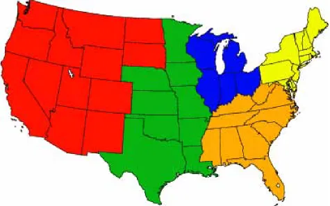
Figure 1. The CMAQ modeling domain. The black, red, and blue boxes denote domains over the 36-km continental US, the 12-km western US, and the 12-km eastern US, respectively (filled yellow, orange, blue, green, and red colors denote

operational model performance evaluation for O3, PM2.5

and its speciated components such as SO4 2

, NO3

 ,

4, EC, and OC, Hg wet deposition, and a selected set

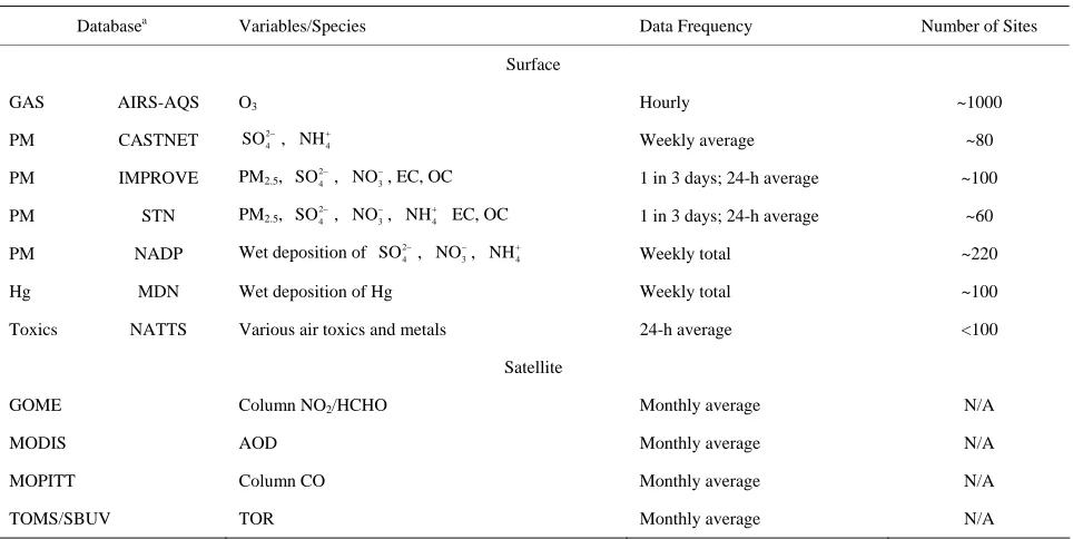
of HAPs is conducted using available routine surface monitoring data and satellite column data (Table 1). The surface data include those from the Clean Air Status and Trends Network (CASTNET), the Interagency Monitor- ing of Protected Visual Environments (IMPROVE), the Speciation Trends Network (STN), the Aerometric In- formation Retrieval System (AIRS)-Air Quality System (AQS), the Southeastern Aerosol Research and Charac- terization study (SEARCH), the National Acid Deposi- tion Program (NADP), the Mercury Deposition Network (MDN), and the National Air Toxics Trends Stations (NATTS). Most of these networks are described in Eder and Yu [10] and Zhang et al. [6].

NH

The satellite column data include the tropospheric CO columns from the Measurements of Pollution in the Tro- posphere (MOPITT) [29], the tropospheric NO2, HCHO

columns, and their ratios (HCHO/NO2) from the Global

Ozone Monitoring Experiment (GOME) [30], the tropo- spheric O3 residuals (TORs) from the Total Ozone Map-

ping Spectrometer/the Solar Backscattered Ultraviolet (TOMS/SBUV) [31], the AOD from the Moderate Reso- lution Imaging Spectroradiometer (MODIS) [32].

In addition to spatial plots, scatter plots, and time se- ries plots, the model performance is examined using sta- tistical metrics that follow Zhang et al. [6] including the

mean bias (MB), correlation coefficient (R), the normal- ized mean bias (NMB), the normalized mean error (NME), and root mean square error (RMSE). The evaluation for surface predictions is conducted primarily using the EPA’s Atmospheric Model Evaluation Tool (AMET). AMET is a software package developed by EPA that can perform the operational evaluation of complex models. The column abundances of CO, NO2, HCHO, O3, and the

ratios of column HCHO/NO2 are calculated using pre-

dicted concentrations from CMAQ and meteorologycal/ domain data (i.e., temperature, pressure, and layer thick-ness) from MM5 and converted into Dobson Unit (DU) for O3 and molecules·cm–2 for other species for com-

parison with satellite data. AODs are estimated based on CMAQ PM2.5 predictions using an empirical equation as

described in Wang et al. [15] and Zhang et al. [8]. In addition, the column mass ratios of HCHO/NO2 simu-

lated by CMAQ-MP are calculated and compared with observed ratios.

3. Evaluation of Model Performance

3.1. Meteorological Variables

Before initiating air quality simulations, it is important to identify the biases and errors associated with meteoro- logical predictions. The MM5 model performance for 2002 MP modeling platform was evaluated separately from this study by Kemball-Cook et al. [25] and Dolwick

Table 1. Summary of observational databases used in the model evaluation.

Databasea _{Variables/Species Data Frequency Number of Sites}

Surface

GAS AIRS-AQS O3 Hourly ~1000

PM CASTNET 2

4 SO, NH4



2 4 SO NO3



2 4 SO NO3



4 NH

Weekly average ~80

PM IMPROVE PM2.5, , , EC, OC 1 in 3 days; 24-h average ~100

PM STN PM2.5, , ,



EC, OC 1 in 3 days; 24-h average ~60

PM NADP Wet deposition of 2 ,

4

SO NO3 NH4



,  Weekly total ~220

Hg MDN Wet deposition of Hg Weekly total ~100

Toxics NATTS Various air toxics and metals 24-h average <100

Satellite

GOME Column NO2/HCHO Monthly average N/A

MODIS AOD Monthly average N/A

MOPITT Column CO Monthly average N/A

TOMS/SBUV TOR Monthly average N/A

a_{AIRS-AQS: Aerometric Information Retrieval System-Air Quality Subsystem; CASTNET: Clean Air Status and Trends Network; GOME: Global Ozone}

Monitoring Experiment; IMPROVE: Interagency Monitoring of Protected Visual Environments; MDN: Mercury Deposition Network; MODIS: Moderate Resolution Imaging Spectroradiometer; MOPITT: Measurements of Pollution in the Troposphere; NADP: National Acid Deposition Program; NATTS: Na- tional Air Toxics Trends Stations; STN: Speciated Trends Network; TOMS/SBUV: Total Ozone Mapping Spectrometer and the Solar Backscattered Ultravio-

et al. [33]. These evaluations show that the MM5 mete- orological predictions over the three domains represent a good approximation of temperature and water vapor mixing ration with mean biases generally less than 1.5˚C and 0.1 g/kg. The model captures large-scale synoptic patterns such as high-pressure domes and upper-level troughs. However, cold bias of 2˚C - 3˚C on average ex- ists in surface temperature predictions during winter, especially in January, from all three MM5 simulations, which may be due to the limitations of the PBL and land-surface schemes currently used in accurately simu- lating the air-land heat fluxes with the coarse grid resolu- tion [25]. The effect of cold biases is the largest at night, which could overestimate the stability in the lowest lay- ers and have a significant impact on chemical predictions [33]. MM5 is able to replicate the precipitation fairly accurately in spring, fall, and winter, but overestimates it in summer, likely due to the excessive convective cloud predicted by the model [25]. The model biases/errors for various variables over the Rocky Mountain and Great Lakes region are relatively larger than other regions due to complexity of terrains. Overall, the biases and errors associated with these meteorological simulations are

generally within the range of past meteorological model- ing results that have been used for air quality applications [3]. A rigorous performance testing demonstrates that the dynamic and thermodynamic fields generated by MM5 are quite sufficient for the 2002 MP modeling platform [33].

3.2. Criteria Air Pollutants at the Surface

Because of known differences between networks in terms of sampling protocols and measurement procedures, the evaluation for surface chemical predictions is conducted separately for individual network. For each network and pollutant, statistics are calculated for all sites in each domain and also with separate breakouts of five sub- regions (i.e., Midwest, northeast, southeast, central, and west of US) over the CONUS domain (as shown in Fig- ure 1) or observed-predicted data pairs in monthly, sea-sonal, and annual averages. Since the CMAQ evalua- tion results for the 12-km and 36-km grids are fairly con- sistent especially for CAPs (see Table 2), our analyses focus primarily on CMAQ results at 36-km over CONUS in this section unless otherwise noted.

Table 2. Seasonal-mean model performance statistics for criteria air pollutants over CONUS and its 5 other sub-regions from the 36-km simulation and EUS and WUS from the 12-km simulation in 20021.

Winter Spring Summer Fall

Variables Network Sub-Regions

NMB* _{(%) NME}* _{(%) NMB (%) NME (%) NMB (%) NME (%) NMB %) NME (%)}

CONUS 1.5 14.0

Midwest 2.7 13.2

Northeast 1.7 14.2

Southeast 2.6 13.0

Central 3.5 13.0

West –1.2 15.5

EUS (12-km) –1.9 12.9

Max 8-h O3 AIRS-AQS

WUS (12-km) –4.3 15.0

CONUS 29.0 59.5 12.3 48.3 –22.8 34.4 2.4 41.5

Midwest 38.6 49.7 38.4 57.6 –9.1 25.4 15.0 30.3

Northeast 71.8 74.7 35.6 49.8 –17.7 33.2 26.6 43.4

Southeast 21.0 46.8 –2.0 36.0 –29.6 33.7 –8.3 32.7

Central 48.8 65.4 –3.5 50.1 –24.1 37.8 18.3 46.7

West –19.6 57.3 4.1 54.8 –33.4 42.6 –28.2 50.9

EUS (12-km) 47.1 60.2 15.3 46.2 –17.4 33.2 15.5 39.0

STN

WUS (12-km) 2.2 53.5 3.7 50.6 –23.0 38.0 –4.2 46.4

CONUS 74.3 94.0 5.6 53.7 –33.8 48.0 11.4 50.9

Midwest 65.7 70.8 47.2 64.7 –24.2 32.5 29.5 46.7

Northeast 143.9 146.9 47.4 61.0 –28.0 38.7 42.3 57.6

Southeast 47.6 66.5 –1.8 43.3 –33.5 39.9 9.2 42.1

Central 53.4 73.6 –19.1 52.3 –46.1 47.9 16.0 54.1

West 57.0 89.3 –5.7 54.5 –33.7 57.3 –1.5 51.5

EUS (12-km) 55.0 72.2 –1.7 46.9 –38.1 42.9 9.6 42.6

PM2.5 Total Mass

IMPROVE

Continued

CONUS 21.2 56.3 22.5 53.6 –2.3 39.5 2.8 47.7

Midwest 25.6 42.5 52.9 71.7 19.6 38.7 14.0 35.8

Northeast 44.5 51.8 30.0 49.1 3.4 37.9 22.6 44.0

Southeast 33.8 59.3 16.9 44.2 –0.1 34.7 –1.4 39.9

Central 43.4 62.5 11.0 47.0 –5.0 37.3 23.9 53.1

West –33.8 64.6 –0.8 65.9 –42.2 56.2 –42.0 65.5

EUS (12-km) 27.2 47.3 16.9 44.2 1.0 35.0 9.1 39.0

STN

WUS (12-km) –26.8 59.1 –6.1 54.0 –29.1 48.4 –25.8 59.0

CONUS 39.9 47.2 39.9 51.6 –8.7 25.0 16.7 39.0

Midwest 16.8 23.5 63.6 65.7 6.6 20.6 26.8 32.9

Northeast 84.6 84.8 54.0 56.8 –8.6 24.1 26.7 45.9

Southeast 32.8 42.3 15.9 36.4 –16.6 25.6 3.9 35.2

Central 41.4 53.8 7.0 39.9 –8.4 22.7 18.4 38.2

West 45.5 76.4 28.8 50.9 –27.3 43.9 –0.4 53.1

EUS (12-km) 16.8 31.2 24.2 40.5 –11.8 25.3 4.1 29.7

Ammonium (NH4)



2 4 SO

CASTNET

WUS (12-km) –11.2 44.1 –6.2 38.1 –26.0 40.6 –18.2 48.1

CONUS –5.1 38.1 –11.2 35.7 –4.5 32.7 –6.8 36.2

Midwest 3.4 40.9 2.1 37.7 10.0 30.2 –6.2 31.3

Northeast 0.7 32.4 0.5 36.1 1.4 29.7 –4.5 28.4

Southeast –14.5 34.3 –16.0 31.1 –3.0 31.1 –6.8 34.7

Central 1.5 41.6 –24.7 38.5 –12.9 35.3 4.0 43.8

West –24.4 52.2 –16.7 41.6 –42.1 49.6 –38.8 49.2

EUS (12-km) –6.9 35.1 –13.4 35.5 1.6 31.5 –2.8 34.5

STN

WUS (12-km) –8.6 49.2 –14.5 37.4 –27.8 40.6 –22.5 42.8

CONUS 18.1 50.0 –3.1 35.0 –13.6 35.5 –2.9 36.3

Midwest 1.9 43.3 –4.4 29.1 –2.5 29.9 0.9 28.3

Northeast 6.3 35.4 1.5 31.1 –9.5 30.8 –4.2 27.4

Southeast 2.2 36.9 –8.6 31.1 –6.7 35.9 3.9 39.2

Central 4.8 41.7 –24.8 35.7 –26.2 35.3 –8.0 36.9

West 64.3 89.8 8.8 43.2 –19.8 42.2 –6.5 42.1

EUS (12-km) –8.1 36.2 –16.0 32.9 –11.1 32.1 –7.5 32.6

IMPROVE

WUS (12-km) 33.5 61.1 –4.3 38.8 –21.0 41.2 –11.4 38.6

CONUS –0.9 29.2 –10.3 22.0 –9.7 19.7 –4.3 20.2

Midwest –8.3 29.8 –7.7 18.9 –4.8 16.0 –5.9 16.3

Northeast 0.0 24.4 –2.6 17.3 –9.3 16.7 –1.8 15.7

Southeast –2.0 27.3 –14.5 22.3 –6.8 19.8 –1.5 22.2

Central –7.2 24.4 –35.2 35.8 –24.1 27.3 –18.9 24.0

West 46.2 65.2 –7.8 32.0 –35.2 40.7 –12.7 35.8

EUS (12-km) –17.8 25.3 –17.7 23.5 –6.9 17.7 –9.6 20.0

Sulfate ( )

CASTNET

Continued

CONUS 3.6 63.3 38.4 88.5 –27.0 78.1 –4.5 71.2

Midwest 16.6 46.2 79.4 104.9 20.1 89.9 23.2 48.2

Northeast 50.4 67.1 61.5 92.3 5.1 84.5 50.8 91.0

Southeast 37.0 90.9 44.5 116.0 –57.5 76.2 –4.3 78.5

Central 12.0 42.5 46.8 70.0 –8.1 73.8 39.4 65.2

West –49.5 68.1 –22.0 68.5 –64.7 69.3 –54.3 72.7

EUS (12-km) 24.7 56.3 43.2 82.7 –31.8 74.4 14.0 60.0

STN

WUS (12-km) –45.2 59.7 –30.6 59.9 –61.1 69.1 –44.7 65.9

CONUS 54.7 110.2 85.4 139.9 –36.8 96.3 50.7 112.9

Midwest 28.6 59.0 168.0 194.5 –6.4 96.1 56.6 75.6

Northeast 181.9 192.5 196.6 221.0 26.2 128.2 160.0 191.7

Southeast 65.0 117.5 92.8 161.1 –37.3 96.4 76.1 146.1

Central 29.5 74.1 58.8 116.1 –65.2 82.9 61.7 96.5

West 3.5 95.2 38.6 103.9 –47.3 92.2 11.4 98.4

EUS (12-km) 50.1 95.7 89.1 140.9 –43.8 95.3 53.2 100.5

Nitrate (NO3)



IMPROVE

WUS (12-km) –38.7 74.0 –22.6 79.1 –73.3 88.6 –16.1 84.4

CONUS 20.6 68.0 –3.8 58.7 –14.3 64.6 –7.2 57.6

Midwest 21.3 40.9 –11.9 32.4 –40.0 43.0 –7.1 33.8

Northeast 69.1 82.1 23.7 48.8 –30.3 49.9 9.7 46.5

Southeast –3.0 42.8 –21.0 41.3 –43.2 48.1 –24.4 39.0

Central 3.8 51.0 –33.4 39.4 –43.5 49.5 –2.0 47.6

West 9.1 78.9 28.6 79.3 4.9 77.9 –8.5 71.1

EUS (12-km) 10.4 53.5 –13.4 44.5 –40.1 52.2 –13.5 45.2

Elemental Carbon

(EC) IMPROVE

WUS (12-km) –7.4 70.5 –2.6 62.4 –22.8 65.5 –15.2 69.7

CONUS 45.3 84.1 –2.2 60.4 –41.7 64.7 –11.9 54.2

Midwest 25.0 53.6 –20.8 41.8 –68.5 68.9 –36.3 41.9

Northeast 115.1 128.1 31.1 53.2 –61.2 65.8 17.9 46.3

Southeast 3.2 47.6 –32.9 55.3 –67.9 68.5 –34.9 46.4

Central 11.7 57.1 –46.0 55.7 –71.0 71.4 –31.5 50.2

West 42.4 90.3 13.7 67.8 –25.7 62.5 –8.1 59.1

EUS (12-km) 24.6 65.4 –27.2 53.1 –66.8 69.0 –25.5 47.2

Organic Carbon

(OC) IMPROVE

WUS (12-km) –2.9 59.9 –23.7 54.5 –50.4 63.7 –29.5 56.6

CONUS –16.4 54.1 –16.5 51.5 –57.8 61.2 –37.5 50.7

Midwest –6.0 55.3 –13.7 51.7 –61.2 62.3 –35.7 43.6

Northeast 23.5 51.3 4.7 44.5 –60.1 63.7 –14.7 39.2

Southeast –28.4 44.2 –23.1 47.8 –63.5 64.2 –44.3 52.1

Central –12.3 46.6 –29.0 49.0 –54.9 59.5 –35.7 47.4

STN

West –38.0 66.5 –15.8 63.1 –48.2 54.6 –46.9 60.6

CONUS 40.2 78.5 –0.1 58.2 –38.3 63.2 –11.0 51.9

Midwest 24.1 49.2 –18.8 38.2 –63.8 64.0 –29.6 36.2

Northeast 104.5 115.8 29.8 50.5 –56.9 61.5 16.2 43.0

Southeast 2.0 45.0 –30.8 52.2 –64.6 65.3 –33.0 43.4

Central 10.3 55.1 –43.9 51.9 –67.3 67.8 –26.5 48.1

Total Carbon (TC)

IMPROVE

West 35.8 85.0 16.3 67.1 –22.2 62.5 –8.1 57.7

1_{Winter: Jan., Feb., and Dec.; Spring: Mar., Apr., and May; Summer: Jun., Jul., and Aug, for other species and May to Sep. for O}

2

SO

3.2.1. Ozone the O3 season binned for the range of observed O3 values.

CMAQ tends to reproduce O3 mixing ratios the best in

the range of 40 - 60 ppb with MBs within 5 ppb but sig- nificantly underpredicts high mixing ratios (>80 ppb) and overpredicts low mixing ratios of O3 (<40 ppb). Those

observed low O3 mixing ratios typically coincide with

non-conducive meteorological conditions (e.g., high cloud cover and precipitation and cool temperature). The over-estimation of low observed mixing ratios of O3 is due in

part to the poor performance of CMAQ in simulating the nighttime O3 as discussed above. As shown in Tables 2

and 3, CMAQ shows overall excellent performance with very small domain-wide NMBs of 1.5%, 1.7%, 2.6%, 2.7%, 3.5%, and –1.2% for CONUS and its subregions including northeast, southeast, Midwest, central, and west US, respectively, during O3 season. The NMBs are

–1.9% over EUS and –4.3% over WUS from the 12-km simulations. Although the discrepancies still exist for modeled and observed O3 mixing ratios, the results in

this study demonstrate a moderate to significant im-provement as compared with previous studies [8,10,12, 36] because of several factors. First, a relatively new ver- sion of CMAQ v4.6 with the newest CB05 chemical me- chanism plus additional chloride reactions is used. Re- cent studies by Luecken et al. [37] and Yu et al. [38] showed that CB05 performs better in reproducing high O3 mixing ratios, especially in summer when compared

with CB-IV and Statewide Air Pollution Research Center mechanism (SAPRC99) due to several updates in che- mical species, reactions, and reaction rates. Second, a new option of PBL scheme, ACM2, is available in CMAQ v4.6 and used in this study. ACM2 includes both eddy diffusion and nonlocal schemes from the original ACM, which enables ACM2 to better represent the rise and fall of the convective boundary layer. Appel et al. [12] also compared O3 performance of CMAQ v4.5 with

CMAQ v4.6 both with CB05 and found a better overall performance for max 8-h O3 by CMAQ v4.6, potentially

due to the use of ACM2. Finally, the emission inventory used in this work is based on NEI 2002 v3, which repre- sents the most comprehensive emission inventory upon its release and is more accurate than those used in previ- ous studies.

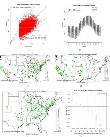
Figure 2(a) shows scatter plot of modeled and observed daily max 8-h O3 with a cut off value of 40 ppb (i.e., data

pairs containing observed mixing ratios less or equal to 40 ppb are not used in the analysis) for the O3 season (i.e.,

May to September). As shown, CMAQ simulates max 8-h O3 mixing ratios quite well with R, NMB, and NME

of 0.7%, 1.5%, and 14%, respectively and a vast majority of values within a factor of 1.5 of observations. Figure 2(b) shows the box plot of 25% and 75% quartiles (shading regions) along with the median values for diur- nal O3 values during the entire O3 season at the AQS

sites (i.e., urban and suburban areas) across the entire domain. As shown, the median simulated O3 values are

fairly close to observations between 10:00 and 19:00, de- spite a systematic overprediction of nighttime and early morning O3. These findings are consistent with previous

studies [10,12]. Although the capability of CMAQ in simulating nighttime O3 has been improved with an

up-dated parameterization of the minimum KZ since CMAQ

v4.5 (see release note at

http://www.cmascenter.org/help/model_docs/cmaq/4.5/R ELEASE_NOTES.txt), accurately simulating the evolu- tion of nocturnal boundary layer remains difficult due to limitations of PBL and land-surface schemes in current models, and the use of a coarse horizontal resolution and vertical resolution in lower portion of PBL (e.g., ~38 m in depth for surface layer in this work).

Figures 2(c)-(e) show the spatial distribution of NMBs for max 8-h O3 with a cutoff value of 40 ppb over the

CONUS at 36-km and WUS and EUS domains at 12-km for the O3 season in 2002. For CONUS at 36-km, CMAQ

shows a good performance to capture the spatial varia-tion of max 8-h O3 mixing ratios with NMBs of within

±10% and NMEs of less than 15% over majority (>80%) of AQS sites based on the suggested performance criteria by other studies [6,34]. CMAQ tends to moderately over- predict O3 mixing ratios along some coastal regions with

NMBs of 20% - 30% (e.g., New England coast and Flor-ida coast) and sometimes >30% (e.g., along Pacific coast in California). This can be attributed to a poor represen-tation of coastal boundary layers [35,36]. There are also several small clusters of overpredictions (with NMBs

20%) in the Midwest and southeastern US and a cluster of underpredictions (with NMBs of –25% to –15%) in some areas in southern California and Arizona. These large NMBs are likely due to the fact that the use of a coarse grid resolution of 36-km cannot accurately repre- sent precursor emissions and elevated and/or complex terrains over those regions. As shown in Figures 2(d)-(e), the simulations at 12-km over WUS and EUS give lower NMBs over those regions (e.g., NMBs of –10% - 0% in most of the two domains).

3.2.2. PM2.5 and Its Compositions

3.2.2.1. Sulfate

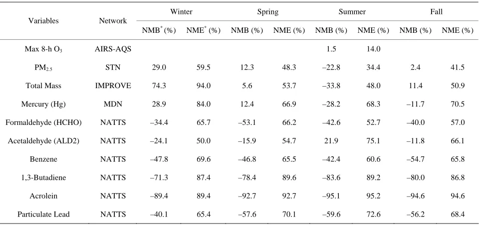
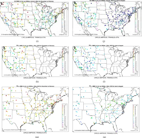
Figures 3(a)-(b) show the spatial plots of NMBs for

4



over the IMPROVE, STN, and CASTNET sites for winter (Jan., Feb., and Dec.) and summer (Jun., Jul., and Aug.) 2002 from the 36-km simulations over CONUS. In both winter and summer, CMAQ performs better over the eastern US than the western US with most of NMBs within ±20%. This is especially true in

O3

O3

(a) (b)

O3

O3

(c) (d)

O3

O3

(e) (f)

Figure 2. Comparison of the simulated and observed O3 concentrations at the AIRS-AQS monitoring sites during O3 season

(i.e., May to September) in 2002. (a) Scatter plot of daily max 8-h O3 with a cut off value of 40 ppb (the 1:1, 1.5:1 and 1:1.5

lines are shown for reference); (b) Box plot of diurnal variation of median (the cross sign denotes AQS and the triangle sign denotes CMAQ) and inter-quartile ranges (light and dark shading denote AQS and CMAQ, respectively) for hourly average O3; Spatial distributions of NMBs for daily max 8-h O3 from (c) The 36-km simulation over CONUS, and the 12-km simula-

Table 3. Seasonal-mean model performance statistics for max 8-h O3, PM2.5, and selected hazardous air pollutants over

CONUS in 20021.

Winter Spring Summer Fall

Variables Network

NMB* _{(%) NME}* _{(%) NMB (%) NME (%) NMB (%) NME (%) NMB (%) NME (%)}

Max 8-h O3 AIRS-AQS 1.5 14.0

PM2.5 STN 29.0 59.5 12.3 48.3 –22.8 34.4 2.4 41.5

Total Mass IMPROVE 74.3 94.0 5.6 53.7 –33.8 48.0 11.4 50.9

Mercury (Hg) MDN 28.9 84.0 12.4 66.9 –28.2 68.3 –11.7 70.5

Formaldehyde (HCHO) NATTS –34.4 65.7 –53.1 66.2 –42.6 52.7 –40.0 57.0

Acetaldehyde (ALD2) NATTS –24.1 50.0 –15.9 54.7 21.9 75.1 –11.8 66.1

Benzene NATTS –47.8 69.6 –46.8 65.5 –42.4 60.6 –54.7 65.8

1,3-Butadiene NATTS –71.3 87.4 –78.4 89.6 –83.6 89.2 –80.0 86.8

Acrolein NATTS –89.4 89.4 –92.7 92.7 –95.1 95.2 –94.6 94.6

Particulate Lead NATTS –40.1 65.4 –57.6 70.1 –59.6 72.6 –56.2 68.4

1

Winter: Jan., Feb., and Dec.; Spring: Mar., Apr., and May; Summer: Jun., Jul., and Aug, for other species and May to Sep. for O3; Fall: Sep., Oct., and Nov.; *

NMB: Normalized mean bias; NME: Normalized mean error.

summer when 4 contributes the most to total PM2.5

mass concentrations in the eastern US, likely as the re- sults of a better representation of emissions of SO2 and

in the eastern US. Compared to the 2001 NEI that significantly underestimates SOX emissions in California

(CA) [39] and possibly in other states in the western US during summer, the 2002 NEI showed much higher emissions in those regions in both summer and winter, indicating that the large negative NMBs (–60% to –20%) in predictions in the western US are unlikely caused by underestimation in SOX emissions in summer

but the large positive NMBs (30% - 100%) in this region may be caused by possible overestimation in SOX emis-

sions in winter.

2

SO 



2

SO 

2

SO 

2

SO

2 2

4

SO 

2 4

SO

Table 2 summarizes the overall seasonal statistical performance of CMAQ for all PM2.5 species including

4 over different networks and sub-regions from

three domains (i.e., CONUS, EUS, and WUS). The per- formance for 4 is the best among all PM2.5 species,

with domain-wide NMBs typically within ±18% in dif- ferent seasons in all sub-regions except for regions “Cen- tral” and “West” from the 36-km simulation and the re- gion “WUS” from the 12-km simulation. The NMEs are moderate, ranging from 20% to 50% throughout the year. Several studies that used the 2001 NEI reported that CMAQ v4.4 underpredicted 4 in winter and spring,

overpredicted it in fall, either overpredicted or slightly underpredicted it in summer [8,11,13]. In contrast, our results show that CMAQ underestimates SO4

timates it over the IMPROVE sites in winter, which are more consistent with the study of Luo et al. [40] that used CMAQ v4.7. This discrepancy is likely due to the updates in both convective cloud module and aerosol dry deposition module in CMAQ v4.6. Appel et al. [13] in- dicated that the use of ACM2-cloud scheme (in CMAQ v4.6 or later) over the RADM-cloud scheme (in CMAQ v4.4) may result in less aqueous production of 4

2

SO

and the changes in aerosol dry deposition calculation in the new version of CMAQ may lead to higher dry depo- sition velocity and hence more SO4 removal. More-

over, the CMAQ model bias in this study can be partially explained by the errors of MM5 in the predictions of precipitation and wet depositions. For example, MM5/ CMAQ tends to overestimate domain-wide precipitation and wet deposition of 4 with NMBs of 42.5% and

13.1%, respectively, in summer and underestimate them with NMBs of –13.0% and –31.1%, respectively, in win- ter (figures not shown). Further, Luo et al. [40] reported that the convective precipitating cloud fraction and cloud water contents have been overestimated by CMAQ v4.6, which leads to an excessive scavenging of

2

2

SO

2 4

SO .

3.2.2.2. Nitrate

Similar spatial plots of NMBs for 3 at the IM-

PROVE and STN sites are shown in Figures 3(c)-(d). In winter, CMAQ tends to overpredict 3 concentra-

tions in the eastern US where NMBs often exceed 20% and it tends to underpredict in most of the western US. In summer, underpredictions of 3 occur over almost

ll the CONUS domain. As shown in Table 2, CMAQ

NO

NO

NO



SO4

SO4

(a) (b)

NO3

NO3

(c) (d)

NH4

NH4

(e) (f)

(i) (j)

PM2.5

PM2.5

(k) (l)

PM2.5

PM2.5

(m) (n)

Figure 3. Spatial plots of NMBs for 2 ((a) and (b)),

4

SO NO3



((c) and (d)), NH4 

((e) and (f)), EC ((g) and (h)), and OC ((i) and (j)) from the 36-km simulation over CONUS, and PM2.5 ((k)-(n)) from the 12-km simulation over WUS and EUS for

win-ter (left panel) and summer (right panel) 2002.

performance for 3 is much worse than that for

4 . NMBs and NMEs are much larger. Domain-wide

NMBs and NMEs can be up to 85.4% and 139.9%, re- spectively. The model biases may be partially associated with the uncertainties in NH3 emissions, which are more

rudimentary than those of other species such as NOX,

particularly in its monthly variation that is poorly char- acterized [41]. Model performance with respect to 3

NO

2

SO 

NO

2002 NEI v3. The more accurate monthly-derived NH3

emissions by Carnegie Mellon University NH3 emission

model are much higher in summer and lower in winter compared to the traditional NH3 emission inventories

[14,42] and can be used to improve model performance in the future. Other important reasons include the high uncertainties in gas/particle partitioning simulated by ISORROPIA in CMAQ and the biases in the predictions

of 3



in this study suggests that NH3 emissions based on the

2002 NEI v3 are probably too low for summer and too high for other seasons, which was reported for previous versions of NEI in the literature [6] but remains in the

NO wet deposition fluxes. CMAQ tends to under- estimate the NO3



tively. Finally, the large model biases and errors in NO3



predictions could also be due in part to the uncertainties in the measurements, especially in summer. In fact, both modeled and observed NO3



concentrations are very low in summer and the model biases are comparable to the uncertainty level (roughly ±0.5 μg·m–3) of filter-based routine measurements [43].

3.2.2.3. Ammonium

As shown in Figures 3(e)-(f), since 4 in the am-

bient atmosphere is generally present as (NH4)2SO4 (or

NH4HSO4) and NH4NO3, the spatial pattern of

NH

4

NH is

more like the combined pattern of and 3 2

4

SO  NO in

winter when both (NH4)2SO4 and NH4NO3 concentra-

tions are high and more similar to that of 4 2

SO  in sum- mer when (NH4)2SO4 is dominant. In winter, CMAQ

overpredicts 4 concentrations in the eastern US

where NMBs often range from 20% to 60%. It underpre- dicts NH4+ concentrations in the most of the western US,

where NMBs range from –60% to –20%. In summer, CMAQ shows a better performance over space, with slight overpredictions of 4 over the eastern US

(with most NMBs of 0 to 40%) and slight underpredic- tions over the western US (with most NMBs of –40% to –20%), because is dominant by (NH4)2SO4 and

the performance of in summer is much better than that of 3 in winter. Table 2 shows a fairly good

performance for 4 , which is slightly worse than

but better than 3. The domain-wide NMBs

and NMEs range from –2.3% to 39.9% and 25.0% to 56.3%, respectively, over different networks in different seasons. The statistics are consistent between STN and CAST-NET, with domain-wide positive NMBs in most seasons except for summer over both networks. As dis-cussed above, the uncertainty associated with NH3

emis-sions is indicative of the main reason for the model bias of 4 . Additionally, the underestimation of 4

NH   NH NH NH  NO  4  2 4 SO  NH NO 2 4 SO 

NH 

wet depositions throughout the whole year (NMBs are –47.5%, –26.4%, –8.9%, and –22.2% for winter, spring, summer, and fall, respectively) can explain in part the overestimation of NH4+ in most seasons.

3.2.2.4. Elemental and Organic Carbon

As shown in Figures 3(g)-(h), CMAQ moderately over- predicts EC at the IMPROVE and STN sites in the east- ern US with NMBs generally between 20% and 50% and underpredicts it in the western US with NMBs between –50% and –20% in winter. As shown in Figures 3(i)-(j), CMAQ has the tendency to overpredict OC over the western US, Midwest, and New England areas especially for the IMPROVE sites. Underpredictions are also evi- dent over most STN sites in the eastern US. While in summer, significant underpredictions are observed across the whole domain, particularly over the eastern US and the worst NMBs normally occurring over the STN sites.

The model seems to perform slightly better in winter (colder months) than summer (warmer months).

ment techniques of carbonaceous aerosols (e.g., OC and EC split) and the factor used to convert simulated organic matter (OM) to OC may also cause the discrepancies be- tween simulations and observations [13].

3.2.2.5. PM2.5

The accuracy of PM2.5 predictions in CMAQ is a com-

posite of the accuracies of predictions of individual par- ticulate species concentrations. Figures 4(a)-(b) and 3(k)- (n) show the spatial plots of NMBs for PM2.5 at the IM-

PROVE and STN sites from the 36-km simulation over CONUS and the 12-km simulations over WUS and EUS, respectively. CMAQ overpredicts PM2.5 in winter and

underpredicts it in summer for all domains. In winter, the spatial variability of biases is more evident. The rela- tively high biases occur over the northeastern US, Great Lakes, and Midwest with NMBs generally >50% at 36-km and >30% at 12-km, indicating some improve- ments using a finer grid resolution of 12-km. The under- prediction of PM2.5 in summer is more systematic with

more than 95% of sites having negative biases. NMBs are typically larger (between –60% and –20%) in the western US than in the eastern US (–40% to –10%) at 36-km, with some improvement at the 12-km.

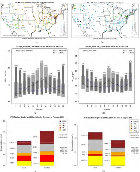
As shown in Figures 4(c)-(d), both CMAQ and ob- servations show higher monthly PM2.5 concentrations at

the STN sites than the IMPROVE sites throughout the year because most of the IMPROVE sites are located in remote and rural areas and the STN sites are located in more polluted urban areas. CMAQ underpredicts PM2.5

concentrations during the warmer months (i.e., April through September at the IMPROVE sites and May through August at the STN sites) but overpredicts during the colder months. Figures 4(e)-(f) show the stacked bar charts of modeled and observed average PM2.5

concen-trations and the contributions of individual species con-centrations (i.e., , 3, 4, total carbon (TC),

and unspeciated PM2.5) to the total PM2.5 concentration at

the STN sites in both winter and summer. In winter, TC is the most abundant (33.2%) PM2.5 component, fol-

lowed by 3 (21.2%), SO (19.8%), other unspe-

ciated PM2.5 (14.3%) and 4 2

4

SO

The reasons for this underprediction were discussed ear- lier in this section. Since the majority of the other unspe- ciated PM2.5 is primary aerosols, the model biases espe-

cially in winter are very likely due to errors in unspeci- ated primary emissions.

As shown in Tables 2 and 3, both NMBs and NMEs are relatively low over most sub-regions. Domain-wide NMBs range from –22.8% (summer) to 29% (winter) over the STN network and from –33.8% (summer) to 74.3% (winter) over the IMPORVE network over CONUS. NMEs are generally lower than 50% at both STN and IMPROVE sites throughout the year except for winter. There are currently no universally-accepted or EPA-re- commended quantitative performance criteria for PM2.5.

However, some specific model performance criteria have been recommended by other modeling studies [6,34]. Generally ±30% for model biases and 50% for model errors can be considered as satisfactory performance and the values below or beyond them should be considered as good and poor performance, respectively. The 2002 MP modeling platform demonstrates an overall good per-formance in predicting PM2.5 except for summer at the

IMPROVE sites and winter at all sites.It also provides comparable or even better performance because of the state-of-science treatments in the model as well as more accurate model inputs.

3.3. Hazardous Air Pollutants at the Surface

3.3.1. Mercury

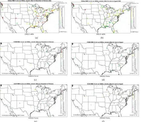
There were no routine networks existing with measure- ments of ambient Hg concentrations and dry depositions over the US back in 2002. MDN established by NADP was the only network that regularly monitored Hg wet deposition with most of its sites scattered throughout the remote areas in the US and Canada. The model evalua- tion will thus focus on the comparison of modeled Hg wet deposition against the MDN measurements, which is considered to be sufficient to provide a general concept of model performance for Hg [22,46]. Only sites where data are available more than half the weeks in a season are utilized for the seasonal performance evaluation in this study. Figures 5(a)-(b) display the spatial variation of NMBs for Hg wet deposition against data from the MDN network for winter and summer 2002. As shown, most MDN sites are clustered in the eastern and Midwest US. In winter, NMBs are much more scattered with NMBs from 10% to 50% occurring over the eastern US and some very high NMBs (>100%) occurring at several sites in both the western and eastern US. Some relatively small negative biases (NMBs of –20% to –10%) are ob- served in the eastern US and large negative biases (NMBs of about –60%) also occur in the Midwest. How-

ver, the overall trend for Hg wet deposition in CMAQ is

NO NH

2 4  NH NO 

(11.6%) from the STN observations. However, CMAQ predicts the highest other unspeciated PM2.5 (36.7%), which contributes to the most

to the PM2.5 overprediction in winter. The agreement be-

tween predicted and observed PM2.5 concentrations with-

out accounting for the contribution of other unknown PM2.5 would be considerably better with a slight positive

bias from CMAQ. In summer, both TC (34.2%) and (29.9%) are the dominant PM2.5 component, fol-

lowing by other PM2.5 (21.2%), 4 (9.9%), and

3 (4.8%) from the STN observations. CMAQ pre-

dicts concentrations of

2 4   SO NO NH 2 4

SO, 4, and other PM2.5

quite well, but significantly underpredicts TC and

NH

3

PM2.5

PM2.5

(a) (b)

PM2.5

PM

2.

5

(

μ

g/

m

3)

PM2.5

PM

2.

5

(

μ

g/m

3)

(c) (d)

(

μ

g/m

3)

 4 NH

 3 NO 2-4 SO

 4 NH  3 NO 2-4 SO

(

μ

g/m

3)

(e) (f)

Figure 4. Comparison of the simulated and observed PM2.5 concentrations at the IMPROVE and STN sites in 2002. Spatial

plots of NMBs from the 36-km simulation over CONUS for winter and summer in 2002 ((a) and (b)); Monthly box plot for total PM2.5 concentrations with 25% and 75% quartiles and median values over (c) the IMPORVE sites; and (d) the STN

sites in 2002 (triangle and dark shading denote CMAQ, square and light shading denote observations, and the numbers above each bar indicate the number of simulated/observed data pairs for each month); Stacked bar charts of total mass con- centrations of PM2.5 and its major components over the STN sits for (e) winter; and (f) summer in 2002. The percentages

(a) (b)

(c) (d)

(e) (f)

Figure 5. Spatial plots of NMBs for Hg wet deposition (top), formaldehyde mixing ratio (middle), and acetaldehyde mixing ratio (bottom) for winter (left panel) and summer (right panel) 2002.

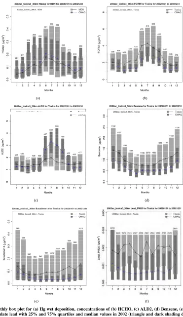
an overprediction in winter. In summer, the Hg wet deposition is generally underpredicted at more than 80% of the MDN sites, especially over the southern US with NMBs of –70% to –10%. For annual predictions of Hg wet deposition fluxes, more than half of data pairs are within the factor of 2 reference lines (figure not shown) with an R value of 0.45. As shown in Table 3 and Fig- ure 6(a), CMAQ does reasonably well in simulating the monthly and seasonal Hg wet deposition over CONUS, with domain-wide seasonal NMBs of –28.2% to 28.9% and NMEs of 66.9% - 84.0%. The model performance is slightly better in spring and fall than in summer and win- ter.

The evaluation results of the present study are more in line with those from Gbor et al. [46] and Bullock et al. [18], and, show an improvement over those reported by Bullock and Brehme [22]. The Hg wet depositions in

Bullock and Brehme [22] were significantly overpre- dicted for summer with an NMB of 60.2% and moder- ately overpredicted for spring with an NMB of 25.9%, compared to –28.2% and 12.4% in this study for summer and spring, respectively. The performance for precipita- tion is very similar between the two studies. The im- provement of model performance is thus more likely related to the science updates in CMAQ-MP. These up- dates include: 1) The modification of the products and reaction rates for reactions of Hg0 with hydrogen perox- ide (H2O2), O3, and hydroxyl radical (OH); 2) The ex-

(

μ

g/m

2)

(

μ

g/m

3)

(a) (b)

(

μ

g/

m

3)

(

μ

g/m

3)

(c) (d)

(

μ

g/

m

3)

(

μ

g/m

3)

(e) (f)

Figure 6. Monthly box plot for (a) Hg wet deposition, concentrations of (b) HCHO, (c) ALD2, (d) Benzene, (e) Butadiene13, and (f) Particulate lead with 25% and 75% quartiles and median values in 2002 (triangle and dark shading denote CMAQ,

ture [18]. Despite the model improvement, there still in CMAQ, should not occur under ambient conditions.

e, including HCHO, n be generated or exist large discrepancies between CMAQ and MDN ob-

servations. The wet deposition of Hg is directly deter- mined by the precipitation amount simulated by MM5 and the aqueous-phase concentrations of dissolved Hg(II) and absorbed PHg simulated by CMAQ. The model bi- ases in Hg wet deposition predictions are thus deter- mined by the errors in predicting those variables. How- ever, as shown in the previous section, MM5 underpre- dicts precipitation in winter but overpredicts it in summer, which cannot help explain the overprediction of Hg wet deposition in winter and underprediction in summer. This means that the discrepancies between model and obser- vations are more likely due to the predicted Hg(II) and PHg concentrations, which can be further attributed to the uncertainties in emission inputs, BCONs, and Hg chemistry treatments in the model. For example, as indi- cated by Gbor et al. [46], most modeling studies on Hg in the US have excluded a detailed treatment of Hg emis- sions from natural sources including vegetation, soil, and water. They estimated that the total natural mercury emission was 230 tons in 2002 based on their Hg natural emission model, while the anthropogenic emission was 126 tons based on the 1999 NEI. The total Hg emissions from the 2002 NEI are only 112 tons (the US EPA 2002 NEI booklet) which is predominated by anthropogenic emissions. Although the natural Hg emissions based on a modified Biogenic Emission Inventory System (BEIS) model [48] are also included in the 2002 MP modeling platform, the estimation may still be too low, especially, since Lin et al. [48] estimated that Hg emissions from vegetation ranged from 31 to 127 tons with the best es- timation of 44 tons in 2001. This underestimation of natural Hg emissions is much more evident in the sum- mer season during which meteorology, vegetation, and soil conditions favoring the generation of Hg emissions. A recent study by Pongprueksa et al. [17] showed that response of CMAQ to change of BCONs of Hg species, particularly Hg0, was strongly linear and they found an average of 1 ng·m–3 of Hg0 in BCONs could result in an increase of 0.81 ng·m–3 in the monthly average total Hg concentrations and 1270 ng·m–2 in the monthly average total deposition compared with clean condition of Hg0. This indicates that the uncertainties embedded in GEOS- Chem Hg simulation may contribute significantly to CMAQ predictions. Bullock et al. [18] also showed that CMAQ-Hg with BCONs from another CTM gave better performance than those from GEOS-Chem. It is known that the majority of Hg wet deposition are attributable to dissolved Hg(II), thus an accurate estimation of their concentrations is essential for accurate Hg wet deposition predictions. Gardfeldt and Jonsson [49] argued that Hg(II) reduction by HO2 in aqueous-phase chemistry, which is

the most important chemical removal pathway for Hg(II)

Lin et al. [16] and Pongprueksa et al. [17] tested this

assumption by replacing the aqueous Hg(II)-HO2

reduc-tion in CMAQ by two other different gas-phase reducreduc-tion pathways (i.e., Hg(II) reduction by CO or photochemi-cal-reduction of Hg(II)) separately. They found that those two new pathways generated more Hg wet deposition in summer and produced significantly better model agree- ment with the wet deposition measured by the MDN network. Finally, the missing reactions of Hg with other oxidants, such as bromines, in CMAQ may also contrib-ute to the model uncertainties [50].

3.3.2. Other Air Toxics Compounds

1) There are two groups of gaseous HAPs species treated in CMAQ-MP. The first on

ALD2, 1,3-butadiene, and acrolein, ca

destroyed and then influence the concentrations of O3

and radicals via reactions. The second one, including the rest of species and serving as tracers, is only destroyed via chemical reactions with O3 and radicals but does not

alter the concentrations of those oxidants. A modeling approach analogous to tracers in the gas-phase is used for the aerosol-phase HAPs such as diesel PM, lead, and chromium. The emissions of primary components of those species are tracked. Similar to EC, they are assumed to be chemically inert and only undergo microphysical and deposition processes, they therefore do not participate in cloud chemistry and have no effects on the rates of those processes (see CMAQ release note,

http://www.cmascenter.org/help/model_docs/cmaq/4.6/H AZARDOUS_AIR_POLLUTANTS.txt). The approach taken above has its limitation. For example, Hutzell and Luecken [21] indicated that the hexavalent and trivalent states of chromium mass exchange might occur through chemistry within cloud droplets. However, the kinetics for that process is not well understood currently and will only be considered for future model development.

2) We therefore select 6 representative and also obser- vationally available species including five gases and one aerosol species to assess the model performance of CMAQ-MP in predicting the HAPs. As shown in Fig- ures 5(c)-(d), CMAQ-MP tends to underpredict HCHO at most NATTS sites in both winter and summer. Similar to the MDN sites, most NATTS sites are located in the eastern US and the model performance evaluation may not be representative for the western US. As shown in

Figures 6(b)-(f) show the monthly concentrations be- tween CMAQ and observations and Table 3 shows the seasonal statistics for HCHO, ALD2, benzene, 1,3-buta- diene, acrolein, and particulate lead. The results show systematic underpredictions for most species except ALD2 throughout the year. No standard performance criteria are recommended by the US EPA and literature for HAPs modeling. Based on performance criteria used for O3 evaluation, the concentrations of HCHO and ben-

zene are moderately-to-significantly underpredicted with NMBs of –53.1% (spring) to –34.4% (winter) for HCHO and –54.7% (fall) to –42.4% (summer) for benzene. That of ALD2 performs much better, with NMBs of –11.8% (fall) to 21.9% (summer). Based on performance criteria used for PM2.5 evaluation, the concentrations of particu-

late lead are also significantly underpredicted with NMBs of –40.1% (winter) to –59.6% (summer). Higher NMBs (generally –90% to –75%) and NMEs (>85%) occur for 1,3-butadiene and acrolein. The model per- formance for all species except for 1,3-butadiene in this study is consistent with or better than that reported by Luecken et al. [23]. For example, they reported NMBs of –52.0% and –39.0% for HCHO, –59.1% and –14.7% for ALD2, –39.1% and –69.8% for benzene, and –56.4% and –55.9% for 1,3-butadiene, for winter and summer, re- spectively. The larger underpredictions in the concentra- tions of 1,3-Butadiene are likely because that the CB05 mechanism used in this study generates more oxidants than SAPRC99 used by Luecken et al. [23] and includes additional chloride radicals. These additional oxidants and radicals will destroy more 1,3-Butadiene and result in smaller concentrations.

3) Overall, the model performance for HAPs is not as good as that for CAPs. Several factors may contribute to large model biases (mostly underpredictions) for HAPs. First, the grid resolution used in this study may be too co

del performance of the 2002 MP modeling plat- ther examined by evaluating predictions against available tellite measurements can

in 20

arse to resolve the sub-grid phenomena (such as urban canopies and sub-grid plumes) frequently associated with many HAP species as reported by other studies [51-53]. For example, Logue et al. [53] reported that most of air toxics compounds measured around Pittsburgh areas were characterized by short periods of elevated concen- trations or plume events. Some local sources of emis- sions (e.g., HCHO) and the highly-reactive precursors (e.g., 1,3-butadiene with only a few hours of lifetime) may impact the monitors but not be captured in the grid average model predictions [23]. Ching et al. [51] also found that CMAQ predictions of air toxics are generally better (i.e., with higher values) at a horizontal grid reso- lution of 4-km than at 36-km. Second, errors in emission estimations of HAPs may contribute significantly to model biases, especially for those chemically nonreactive species (e.g., benzene and various metal particles). As indicated by Hutzell and Luecken [21], the uncertainties

associated with HAPs emissions in the 2002 NEI are generally larger than those for CAPs. Note that most of HAPs emissions in the 2002 NEI are derived from Toxics Release Inventory (TRI). De Marchi and Hamil- ton [54] reported that the TRI underestimates lead emis- sions by as much as 50% and suggested that it may un- derestimate most other metal HAPs emissions since they normally share similar sources of emissions. Luecken et al. [23] also believed that the underestimation of precur- sor emissions (e.g., isoprene) may contribute to the nega- tive biases for HCHO and ALD2 in CMAQ. Third, the assumption in chemical mechanism and aerosol module for HAPs in the current version of CMAQ-MP as de- scribed earlier in this section may play a role in the model underpredictions. In CB05, the rate of decay for most air toxic tracers is affected by OH and NO3 and it is

difficult to determine how well CB05 reproduces their concentrations due to the lack of observations. In par- ticular, CMAQ-MP performs poorly for those short-live and highly active HAPs (e.g., 1,3-butadiene and acrolein), further investigation of the reactions associated with those species is warranted. Finally, the errors from meas- urements such as sample handling, accuracy of analytical standards, and a lack of site density may also contribute to the model biases, but the impacts of these factors are believed to be smaller as compared with other reasons [55].

3.4. Column Variables

3.4.1. Column Mass of Gases

The mo

form above surface is fur seasonal CMAQ column satellite measurements. The sa

provide substantial additional information with more complete spatial coverage and can also represent better the scale characteristics of model outputs that are aver- aged over a grid cell. The satellite dataset used in this study are all level-3 monthly-averaged data with various resolutions (i.e., 1 × 1.25 for TOMS/SBUV TOR, 1 × 1 for MOPITT CO column, 0.25 × 0.25 for GOME NO2

column, 0.5 × 0.5 for GOME HCHO column, and 1 × 1 for MODIS AOD). The satellite data with different reso- lutions are mapped to the Lambert conformal projection used in CMAQ using the bi-linear interpolation of the NCAR command language. The CMAQ model outputs are also processed and averaged at the same time of sat- ellite overpasses in order to facilitate the comparison.

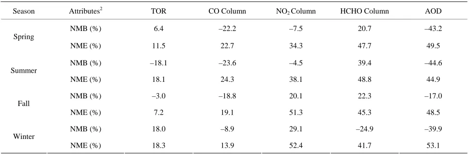
In terms of statistical performance (as shown in Table 4), CMAQ simulates TORs the best in fall and the worst in winter. Figure 7 shows the observed and simulated seasonal-mean TORs over the 36-km CONUS domain

Table 4. Seasonal-mean performance statistics for column predictions over the 36-km CONUS domainin 20021.

Seas_{on Attributes TOR} 2 _{CO Column NO}

2 Column HCHO Column AOD

NMB (%) 6.4 –22.2 –7.5 20.7 –43.2

Spring

NME (%) 11.5 22.7 34.3 47.7 49.5

–18. –23.

Summer

NME (%) 18.1 24.3 38.1 48.8 44.9

NMB (%) –3.0 –18.8 20.1 22.3 –17.0

Fall

NME (%) 7.2 19.1 51.3 45.3 48.5

NMB (%) 18.0 –8.9 29.1 –24.9 –39.9

Winter

NME (%) 18.3 13.9 52.4 41.7 53.1

NMB (%) 1 6 –4.5 39.4 –44.6

1

Th for TOR, CO, NO , and HCHO columns are DU, 1017 molecules·cm–2, 1015 molecules·cm–2, and 10 molecules·cm–2, respectively;

2_{NMB—Normalized m E—Normalize error.}

h west TORs occurred over elevated terrains such as ar-

the 36-km CONUS do

CO columns in winter and spring, especially over the CO

ur on G

and California. Both observed and simulated CO col-

domain in 2002. The spatial distribution and seasonal

e units 2

ean bias; NM

15

d mean

North-eastern, Midwest, and Pacific coastal areas and t e so ce regi s, notably the northeastern US, reat Lakes, lo

eas around Rocky Mountains in the US. CMAQ fails to capture the observed seasonal variations by TOMS/SBUV, i.e., simulated maximum and minimum TORs occur in spring and fall, respectively, but those observed ones occur in summer and winter, respectively. This discrep- ancy might be due to the BCONs for O3 used in CMAQ,

especially in the upper layers that were provided by GEOS-Chem, which make the greatest contribution to TORs [8]. Other possible factors may include the uncer- tainties in both model treatments and the satellite re- trieval algorithms. As pointed out by Tong and Mauzerall [56], the assumption of zero flux at the top layer of the model and the exclusion of the contribution of strato- sphere-troposphere exchange (STE) of O3 limited the

capability of CMAQ to reproduce O3 mixing ratios in the

upper troposphere. Since TORs only represent about 10% of the total O3 columns in the atmosphere, they are

very sensitive to errors in both retrievals of the total O3

column from TOMS and the stratospheric O3 column

from SBUV (Fishman et al., 2003). One of the most im- portant uncertainties in TOMS/SBUV data lies in the definition of tropopause. Stajner et al. [57] indicated that the differences of 1 - 2 km in tropopause altitudes can yield differences of 10% - 20% in tropospheric O3 col-

umns (TOCs). They compared TOCs from four different definitions of tropopause. One of those tropopauses was determined from the lapse rate in the NECP/NCAR re- analysis, which is also used by TOMS/SBUV data. They found that the differences of TOCs from different tro- popause definitions could be up to ~10 DU in summer and ~3 - 4 DU in winter over the US.

Figure 8 shows the observed and simulated seasonal- mean tropospheric CO columns over

main in 2002. Both MOPITT and CMAQ show high

umns are also low over elevated altitude terrains (i.e., Rocky Mountains), which is similar to the TOR results. There are also observed elevated CO columns from MOPITT over the northeastern Pacific coastal region throughout the whole year and with maximum values in spring, which is attributed to the long-range transport of CO [15,58]. Nevertheless, CMAQ underpredicts CO col- umns throughout the whole year with NMBs ranging from –23.6% to –8.9% (see Table 4). CMAQ and MOPITT CO columns are better correlated in fall and summer with R values of 0.76 and 0.62, respectively, de- spite moderate underpredictions. Heald et al. [58] pointed out that the regional emissions, more specifically bio-mass burning emissions, could contribute significantly to elevated CO levels. The uncertainties in CO emissions used in this study could potentially be a major source of errors. The examination of seasonal CO emissions used in CMAQ shows that the CO emissions are the highest in winter, which accordingly contributes to the peak of simulated CO columns. On the other hand, the MOPITT CO observation (peaks in spring) shows that the CO emissions over CONUS, particularly in spring, might be too low. Other possible factors such as uncertainties in BCONs and MOPITT retrieval methods may also con-tribute to the discrepancies between model and satellite. For example, Heald et al. [58] indicated that the model bias in the vertical structure of CO (equivalent with BCONs or profile) could be an important source of model vs. MOPITT discrepancies. Emmons et al. [29] also showed positive biases (19%) of version 3 MOPITT retrievals over continents, as compared to oceans, and the bias may have been increasing over time.

Winter

Spring

Summer

Fall

(a) (b)

Winter

Spring

Summer

Fall

(a) (b)

Winter

Spring

Summer

Fall

(a) (b)

Figure 9. Spatial distributions of seasonal-mean tropospheric NO2 columns from GOME and CMAQ over CONUS in 2002. (a)