Studying the Inter-relationship amongst Possible
Challenges Faced by Woolen Sector in India and other
Asian Countries through ISM and Fuzzy ISM
Methodology
V. K. Aggarwal
Recventures Education Services Private Limited
Delhi, India
S. P. Singh
Department of Management Studies, IIT Delhi,
Delhi, India
Remica Aggarwal
MIT-SOER, MIT- ADT University, Pune, India
ABSTRACT
Present research work focuses on exploring the possible challenges faced by woolen sector in Indian subcontinent and other Asian countries. It further explores the inter-relationship amongst them using ISM Mic-Mac and Fuzzy ISM methodologies.
Keywords
Woolen industry; ISM methodology; Fuzzy ISM methodology
1.
INTRODUCTION
In India, woollen textiles and clothing industry plays a significant role in linking the rural economy with the manufacturing sector represented by small , medium and large scale industries. As per the 2017-18 scenario, India rank third in the sheep population country in the world having 65.07 million sheep producing 43.50 million kg of raw wool . Out of this about 85% is carpet grade wool , 5% apparel grade and remaining 10% coarse grade wool for making rough Kambals etc. Average annual yield per sheep in India is 0.9 Kg. against the world average of 2.4 Kg. A small quantity of specialty fibre is obtained from Pashmina goats and Angora rabbits. The woollen industry in the country is of the size of Rs. 11484.82 crores and broadly divided and scattered between the organized and decentralized sectors. The organized sector consists of composite mills, combing units, worsted and Non worsted spinning units, Knitwears and woven garments units and machine made carpets manufacturing units. The Decentralize Sector includes hosiery and knitting, power-looms, hand knotted carpets, Druggets etc.
There are several woollen units in the country, majority of which are in the small scale sector1. The industry has the potential to generate employment in far-flung and diverse regions and at present provides employment in the organised wool sector to about 12 lakh persons, with an additional 20 lakh persons associated in the sheep rearing and farming sector. Further, there are 3.2 lakh weavers in the carpet sector. The limited wool production in India limits the raw wool requirements of the country. In order to meet the fine quality wool requirement of the organized mills and decentralized hosiery sector , India depends almost exclusively on import.
Following table highlights the major wool producing states along with the quantity of wool produced ( in ‘000 kg) .
S. No. States Wool production 2017-18 (Qty. in ‘000 kg)
1 Rajasthan 13924
2 J& K 7411
3 Karnataka 4392
4 Telangana 4800
5 Gujarat 2267
6 Himachal Pradesh 1500
7 Maharashtra 1418
8 Uttarakhand 558
9 Uttar Pradesh 1404
10 Andhra Pradesh 793
Source : Animal Husbandry Department , Ministry of Agriculture
2.
LITERATURE REVIEW
2.1
Challenges or constraints faced by
woollen sector
2.1.Inadequate and outdated processing facilities (IOPF): The Woolen industry suffers from inadequate and outdated processing facilities. The pre-loom and post-loom facilities are required to be modernized for ensuring quality finished products. Quality finishing of the woolen products will not only increase use of indigenous wool but will also make the product more competitive in the international market.
2.2. Imported machinery incurred huge costs (IM): Due to the overall size of woollen industry and specialized nature of equipment , the industry is dependent on imported plants and machinery. Machinery required for processing from raw wool fibre to fabrics followed by knitting and garmenting, is mostly imported from European countries, USA and Japan.
quality wool to low quality wool in recent years. This is on account of consumer preference for hand tufted carpets in the US and other western markets. Cheap wool import from the Middle East is also constantly growing and is mixed with indigenous wool to make hand tufted carpets.
Other challenges include related to production and marketing of Raw wool .
2.4 Low priority of State Governments (LPG) in development of wool sector.
2.5 Lack of awareness (LoA), traditional management practices, and lack of education and poor economic conditions of woolgrowers.
2.6 Shortage of pasture land (SPL): which force breeders to migrate their flock from one area to another throughout the year.
2.7 Uneconomical return (UR) : of the produces to sheep breeders i.e. sale of raw wool, live sheep, manure, milk, mutton, skin etc.
2.8 Lack of motivation (LoM) : for adopting modern methods of sheep management, machine shearing of sheep, washing & grading of raw wool etc.
2.9 Inadequate production and processing facilities (IPPF) : of specialty fibres i.e. Pashmina goat wool and Angora rabbit wool.
2.10 Inadequate marketing facilities (IMF) and infrastructure
2.11 Ineffective role of state wool marketing organizations (IRMA) : in wool producing States.
2.12 Absence of organized marketing (AOM) : and minimum support price system for ensuring remunerative return.
2.13 Minimum return earned ( MRE) : from sale of wool by wool growers.
(iii) Processing of Wool
2.14 Inadequate dyeing facilities (IDF) : in wool potential areas.
2.15 Need of designing & diversification (NDD) : of woollen handloom products.
2.16 Dearth of technicians & trained manpower (DTTM)
2.17 Inadequate testing facilities (ITF): and quality control measures.
2.18 Inadequate transfer of technology (IToT)
2.19 Lack of operational and technical bench marks (LOTB)
2.20 Lack of education and research (LER) : No educational institute for wool technology resulting lack of expertise in wool sector. This also lead to lesser research opportunities in the field.
2.21 Inadequate database (ID) : Absence of research and education led university or research institute results in inadequate database.
2.22 Lack of R&D work (LR&D)
3.
INTERPRETIVE STRUCTURAL
MODELLING METHODOLOGY
Interpretive structural modelling methodology or ISM [1] is a known technique to map the relationships amongst the relevant elements as per decision maker’s problems in a hierarchical manner. Starting with the identification of elements , it proceeds with establishing the contextual relationships between elements (by examining them in pairs ) and move on towards developing the structural self-interaction (SSIM) matrix using VAXO [14] and then initial reachability matrix and final reachability matrix and rearranging the elements in topological order using the level partition matrices . A Mic-Mac analysis is performed afterwards which categorize the variables as per the driving and dependence power in to autonomous, dependent, driver and linkage category. Finally, a diagraph can be obtained.4.
DEVELOPMENT OF ISM MODEL :
CASE EXAMPLE
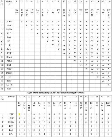
Around 22 challenges described in the above section 2 are being further studied for the possible inter-relationships amongst them. These are Inadequate and outdated processing facilities (IOPF); Need for Imported machinery / huge machinery costs (HMC) ; Shift from high quality wool to low quality wool/ inadequate quality of high wool (IQHW); Low priority of State Governments (LPG); Lack of awareness (LoA) ; Shortage of pasture land (SPL) ; Uneconomical return (UR); Lack of motivation (LoM); Inadequate production and processing facilities (IPPF); Inadequate marketing facilities (IMF) and infrastructure ; Ineffective role of state wool marketing organizations (IRMA) ; Absence of organized marketing (AOM); Minimum return earned (MRE) and Inadequate dyeing facilities (IDF) in wool potential areas; Need of designing & diversification (NDD) ; Dearth of technicians & trained manpower (DTTM); Inadequate testing facilities (ITF) ; Inadequate transfer of technology (IToT) ; Lack of operational and technical bench marks (LOTB) ; Lack of Education and Research (LER); Inadequate database (ID) and Lack of R&D work (LR&D) .
4.1.1 Construction of Structural self- interaction Matrix (SSIM)
This matrix gives the pair-wise relationship between two variables i.e. I and j based on VAXO. SSIM has been presented below in Fig 1.
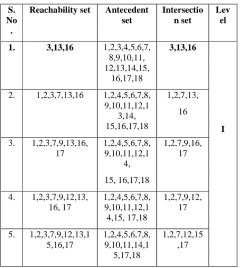
4.1.2 Construction of Initial Reachability Matrix and final reachability matrix
The SSIM has been converted in to a binary matrix called the initial reachability matrix shown in fig. 2 by substituting V, A, X, O by 1 or 0 as per the case. After incorporating the transitivity, the final reachability matrix is shown below in the Fig 3 .
4.2 Fuzzy ISM methodology
4.2.1 Formation of ISM based fuzzy MICMAC analysis model
With the help of key enablers this analysis is done keeping in mind that the relationship amongst enablers would always be equal. However in reality , this may not be true . Some relation may be strong, especially strong and better. To rise above this problem of ISM, fuzzy Mic-Mac analysis is moved away as per following steps:
4.2.3 Binary direct relationship matrix
obtained and the diagonal entries are converted to zero. It has been observed that in the traditional Mic-Mac analysis the relationship is the only binary type, but in this paper fuzzy set theory (FST) is applied to enhance the responsiveness of Mic- Mac analysis. The BDRM is shown in Fig 4. . To convert from traditional Mic-Mac analysis to fuzzy Mic-Mac, a supplementary contribution of option of communication among the enablers is required. The supplementary contribution can be defined by qualitative consideration on
0-1 scale as shown in Table 4.2.3.0-1.
4.2.5 Fuzzy Mic-Mac Stabilized Matrix
After the formation of fuzzy direct relationship matrix (FDRM) as shown in Fig 5 to find the relationship between MCEs, take FDRM as an initial table and repeat the multiplication of matrix until the hierarchies of the driving and dependence power becomes constant. Fuzzy matrix multiplication is based on Boolean matrix multiplication (Kandasamy et al., 2007).
S. No .
Barrier s
1 2 3 4 5 6 7 8 9 10 11 12 13 14 15 16 17 18
IO PF
H M C
IQ H W
LP G
Lo A
S P L
U R
Lo M
IPP F
IR M A
A O M
II/ DF
ND D
DT TM
IQ C M
IT oT
LO TB
LE R & D
1 IOPF V V A A A A A A A A A V A A A A A
2 HMC V A A A A X V A A X X A A V A A
3 IQHW A A A A A A A A A X A A A A A
4 LPG V A V V V V V V V V V V V V
5 LoA O V V V V V V V V V V V V
6 SPL V V V V V V V V V V V V
7 UR V A A A A V A A A A A
8 LoM V A V V V V V V V V
9 IPPF A V V V A V V V A
10 IRMA X V V V V V V V
11 AOM V V A A V V A
12 IIDF O A A V A A
13 NDD A A V A A
14 DTTM V V A V
15 ITF V A A
16 IToT A A
17 LOTB A
[image:3.595.62.540.177.765.2]18 LER
Fig 1: SSIM matrix for pair wise relationship amongst barriers
S. No.
Barriers 1 2 3 4 5 6 7 8 9 10 11 12 13 14 15 16 17 18
IO PF
H M C
I Q H W
LP G
Lo A
S P L
U R
Lo M
IP PF
IR M A
A O M
II/ DF
N D D
D T T M
IQ C M
IT oT
L O T B
LER &D
1 IOPF 1 1 1 0 0 0 0 0 0 0 0 0 0 0 0 0 0 0
2 HMC 0 1 1 0 0 0 0 1 1 0 0 1 1 0 0 1 0 0
3 IQHW 0 0 1 0 0 0 0 0 0 0 0 0 1 0 0 0 0 0
4 LPG 1 1 1 1 1 0 1 1 1 1 1 1 1 1 1 1 1 1
5 LoA 1 1 1 0 1 0 1 1 1 1 1 1 1 1 1 1 1 1
7 UR 1 1 1 0 0 0 1 1 0 0 0 0 1 0 0 0 0 0
8 LoM 1 1 1 0 0 0 0 1 1 0 1 1 1 1 1 1 1 1
9 IPPF 1 0\ 1 0 0 0 1 0 1 0 1 1 1 0 1 1 1 0
10 IRMA 1 1 1 0 0 0 1 1 1 1 1 1 1 1 1 1 1 1
11 AOM 1 1 1 0 0 0 1 0 0 1 1 1 1 0 0 1 1 0
12 IDF 1 1 1 0 0 0 1 0 0 0 0 1 0 0 0 1 0 0
13 NDD 0 1 1 0 0 0 0 0 0 0 0 0 1 0 0 1 0 0
14 DTTM 1 1 1 0 0 0 1 0 1 0 1 1 1 1 1 1 0 1
15 ITF 1 1 1 0 0 0 1 0 0 0 1 1 1 0 1 1 0 0
16 ToT 1 0 1 0 0 0 1 0 0 0 0 0 0 0 0 1 0 0
17 LOTB 1 1 1 0 0 0 1 0 0 0 0 1 1 1 1 1 1 0
[image:4.595.51.548.72.738.2]18 LER 1 1 1 0 0 0 1 0 1 0 1 1 1 0 1 1 1 1
Fig 2: Initial reachability matrix
S. No.
Barri ers
1 2 3 4 5 6 7 8 9 10 11 12 13 14 15 16 17 18 D.P
IO PF
H M C
IQ H W
LP G
Lo A
S P L
U R
Lo M
IP PF
IR M A
A O M
ID F
ND D
DT T M
IT F
To T
LO TB
LE R
1 IOPF 1 1 1 0 0 0 1 1 1 0 0 1 1 0 1 1 1 0 11
2 HMC 1 1 1 0 0 0 1 1 1 0 1 1 1 1 1 1 1 1 13
3 IQH
W
0 0 1 0 0 0 0 0 0 0 0 0 1 0 0 1 0 0 3
4 LPG 1 1 1 1 1 0 1 1 1 1 1 1 1 1 1 1 1 1 17
5 LoA 1 1 1 0 1 0 1 1 1 1 1 1 1 1 1 1 1 1 16
6 SPL 1 1 1 1 1 1 1 1 1 1 1 1 1 1 1 1 1 1 18
7 UR 1 1 1 0 0 0 1 1 1 0 1 1 1 1 1 1 1 1 14
8 LoM 1 1 1 0 1 0 1 1 1 1 1 1 1 1 1 1 1 1 16
9 IPPF 1 1 1 0 0 0 1 0 1 0 1 1 1 1 1 1 1 0 12
10 IRM A
1 1 1 0 0 0 1 1 1 1 1 1 1 1 1 1 1 1 15
11 AO M
1 1 1 0 0 0 1 1 1 1 1 1 1 1 1 1 1 0 11
12 IDF 1 1 1 0 0 0 1 0 1 0 0 1 1 1 0 1 1 0 10
13 NDD 1 1 1 0 0 0 1 0 0 0 0 0 1 0 0 1 0 0 6
14 DTT M
1 1 1 0 0 0 1 0 1 0 1 1 1 1 1 1 1 1 13
15 ITF 1 1 1 0 0 0 1 0 1 0 1 1 1 0 1 1 1 0 10
16 ToT 1 1 1 0 0 0 1 1 1 0 0 0 1 1 0 1 1 0 10
17 LOT B
1 1 1 0 0 0 1 1 1 0 1 1 1 1 1 1 1 0 12
18 LER 1 1 1 0 0 0 1 1 1 0 1 1 1 1 1 1 1 1 14
De.P 17 17 18 2 4 1 17 12 16 6 13 15 18 14 14 18 16 9
Fig 3 : Final reachability matrix
1 2 3 4 5 6 7 8 9 1 0
11 12 13 14 15 16 17 18
IO P F
H M C
IQH W
LP G
Lo A
SP L
UR LoM IP
PF I R M A
AO M
ID F
ND D
DT TM
ITF To T
LO TB
LE R
1 IOPF 0 1 1 0 0 0 1 1 1 0 0 1 1 0 1 1 1 0
2 HMC 1 0 1 0 0 0 1 1 1 0 1 1 1 1 1 1 1 1
3 IQH W
0 0 0 0 0 0 0 0 0 0 0 0 1 0 0 1 0 0
4 LPG 1 1 1 0 1 0 1 1 1 1 1 1 1 1 1 1 1 1
5 LoA 1 1 1 0 0 0 1 1 1 1 1 1 1 1 1 1 1 1
6 SPL 1 1 1 1 1 0 1 1 1 1 1 1 1 1 1 1 1 1
7 UR 1 1 1 0 0 0 0 1 1 0 1 1 1 1 1 1 1 1
8 LoM 1 1 1 0 1 0 1 0 1 1 1 1 1 1 1 1 1 1
9 IPPF 1 1 1 0 0 0 1 0 0 0 1 1 1 1 1 1 1 0
1 0
IRM A
1 1 1 0 0 0 1 1 1 0 1 1 1 1 1 1 1 1
1 1
AOM 1 1 1 0 0 0 1 1 1 1 0 1 1 1 1 1 1 0
1 2
IDF 1 1 1 0 0 0 1 0 1 0 0 0 1 1 0 1 1 0
1 3
NDD 1 1 1 0 0 0 1 0 0 0 0 0 0 0 0 1 0 0
1 4
DTT M
1 1 1 0 0 0 1 0 1 0 1 1 1 0 1 1 1 1
1 5
ITF 1 1 1 0 0 0 1 0 1 0 1 1 1 0 0 1 1 0
1 6
ToT 1 1 1 0 0 0 1 1 1 0 0 0 1 1 0 0 1 0
1 7
LOT B
1 1 1 0 0 0 1 1 1 0 1 1 1 1 1 1 0 0
1 8
LER 1 1 1 0 0 0 1 1 1 0 1 1 1 1 1 1 1 0
Fig 4: Binary direct reachability matrix
Possibility of reachability No Very low Low Medium High Very high Complete
Value 0 0.1 0.3 0.5 0.7 0.9 1
Fig 5 : Possible Numerical values of reachability
1 2 3 4 5 6 7 8 9 10 11 12 13 14 15 16 17 18
IOP F
HM C
IQ HW
LP G
Lo A
SP L
UR Lo M
IPP F
IR MA
AO M
IDF ND D
DT TM
ITF To T
LO TB
LE R
1 IOPF 0 0.5 0.8 0 0 0 1 1 1 0 0 1 1 0 1 0.6 1 0
2 HMC 1 0 0.8 0 0 0 0.6 0.6 1 0 1 1 0.8 1 1 0.8 1 1
3 IQH W
4 LPG 1 1 1 0 1 0 1 1 1 1 1 1 1 1 1 1 1 1
5 LoA 1 1 1 0 0 0 1 1 1 1 1 1 0.7 1 1 0.6 1 1
6 SPL 1 1 1 1 1 0 1 1 1 1 1 1 1 1 1 1 1 1
7 UR 1 1 1 0 0 0 0 1 1 0 1 1 0.7 1 1 0.7 1 1
8 LoM 1 1 1 0 1 0 1 0 1 1 1 1 1 1 1 1 1 1
9 IPPF 1 1 1 0 0 0 1 0 0 0 1 1 0.7 1 1 0.7 1 0
10 IRM A
1 1 1 0 0 0 1 1 1 0 1 1 1 1 1 1 1 1
11 AOM 1 1 1 0 0 0 1 1 1 1 0 1 1 1 1 1 1 0
12 IDF 1 1 1 0 0 0 1 0 1 0 0 0 1 1 0 0.6 1 0
13 NDD 1 1 1 0 0 0 1 0 0 0 0 0 0 0 0 1 0 0
14 DTT M
1 1 1 0 0 0 1 0 1 0 1 1 1 0 1 0.8 1 1
15 ITF 1 1 1 0 0 0 1 0 1 0 1 1 1 0 0 1 1 0
16 ToT 1 1 1 0 0 0 1 1 1 0 0 0 1 1 0 0 1 0
17 LOT B
1 1 1 0 0 0 1 1 1 0 1 1 1 1 1 1 0 0
18 LER 1 1 1 0 0 0 1 1 1 0 1 1 1 1 1 1 1 0
Fig 6 : Fuzzy direct reachability matrix
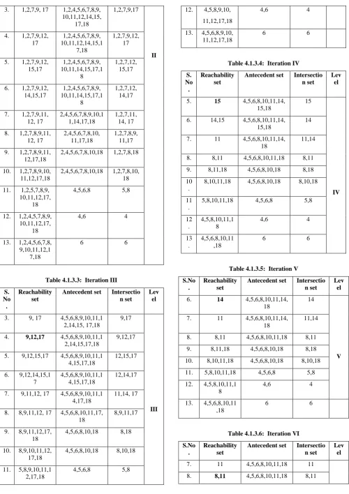
4.1.3 Level Partition
[image:6.595.48.291.497.765.2]From the final reachability matrix, reachability and final antecedent set for each factor are found. The elements for which the reachability and intersection sets are same are the top-level element in the ISM hierarchy. After the identification of top level element, it is separated out from the other elements and the process continues for next level of elements. Reachability set, antecedent set, intersection set along with different level for elements have been shown below in table 1.
Table 4.1.3.1: Iteration I
S. No .
Reachability set Antecedent set
Intersectio n set
Lev el
1. 3,13,16 1,2,3,4,5,6,7, 8,9,10,11, 12,13,14,15,
16,17,18
3,13,16
I
2. 1,2,3,7,13,16 1,2,4,5,6,7,8, 9,10,11,12,1
3,14, 15,16,17,18
1,2,7,13,
16
3. 1,2,3,7,9,13,16, 17
1,2,4,5,6,7,8, 9,10,11,12,1
4,
15, 16,17,18
1,2,7,9,16, 17
4. 1,2,3,7,9,12,13, 16, 17
1,2,4,5,6,7,8, 9,10,11,12,1 4,15, 17,18
1,2,7,9,12, 17
5. 1,2,3,7,9,12,13,1 5,16,17
1,2,4,5,6,7,8, 9,10,11,14,1 5,17,18
1,2,7,12,15 ,17
6. 1,2,3,7,9,12,13,1 4,15,16, 17
1,2,4,5,6,7,8, 9,10,11,14,1 5,17,18
1,2,7,12,14 ,17
7. 1,2,3,7,9,11,12,1 3,16, 17
2,4,5,6,7,8,9, 10,11,14,17,
18
1,2,7,11,14 , 17
8. 1,2,3,7,8,9,11,12, 13,16, 17
2,4,5,6,7,8,1 0,11,17,18
1,2,7,8,9,1 1, 17
9. 1,2,3,7,8,9,11,12, 13,16,17,18
2,4,5,6,7,8,
10,18
1,2,7,8,18
10. 1,2,3,7,8,9,10,11, 12,13,16, 17,18
2,4,5,6,7,8,
10,18
1,2,7,8,10, 18
11. 1,2,3,5,7,8,9,10,1 1,12,13,16,17,18
4,5,6,8 5,8
12. 1,2,3,4,5,7,8,9,10 ,11,12,13,
16,17,18
4,6 4
13. 1,2,3,4,5,6,7,8,9, 10,11,
12,13,16,17,18
6 6
Table 4.1.3.2: Iteration II
S. No .
Reachability set
Antecedent set Intersectio n set
Lev el
2. 1,2,7 1,2,4,5,6,7,8,9, 10,11,12,14,
15,17,18
3. 1,2,7,9, 17 1,2,4,5,6,7,8,9, 10,11,12,14,15,
17,18
1,2,7,9,17
II
4. 1,2,7,9,12, 17 1,2,4,5,6,7,8,9, 10,11,12,14,15,1 7,18 1,2,7,9,12, 17
5. 1,2,7,9,12, 15,17 1,2,4,5,6,7,8,9, 10,11,14,15,17,1 8 1,2,7,12, 15,17
6. 1,2,7,9,12, 14,15,17 1,2,4,5,6,7,8,9, 10,11,14,15,17,1 8 1,2,7,12, 14,17
7. 1,2,7,9,11, 12, 17 2,4,5,6,7,8,9,10,1 1,14,17,18 1,2,7,11, 14, 17 8. 1,2,7,8,9,11, 12, 17 2,4,5,6,7,8,10, 11,17,18 1,2,7,8,9, 11,17 9. 1,2,7,8,9,11, 12,17,18
2,4,5,6,7,8,10,18 1,2,7,8,18
10. 1,2,7,8,9,10, 11,12,17,18
2,4,5,6,7,8,10,18 1,2,7,8,10, 18
11. 1,2,5,7,8,9, 10,11,12,17,
18
4,5,6,8 5,8
12. 1,2,4,5,7,8,9, 10,11,12,17,
18
4,6 4
13. 1,2,4,5,6,7,8, 9,10,11,12,1
7,18
[image:7.595.50.551.64.773.2] [image:7.595.301.549.69.445.2]6 6
Table 4.1.3.3: Iteration III
S. No .
Reachability set
Antecedent set Intersectio n set
Lev el
3. 9, 17 4,5,6,8,9,10,11,1 2,14,15, 17,18
9,17
III
4. 9,12,17 4,5,6,8,9,10,11,1 2,14,15,17,18
9,12,17
5. 9,12,15,17 4,5,6,8,9,10,11,1 4,15,17,18
12,15,17
6. 9,12,14,15,1 7
4,5,6,8,9,10,11,1 4,15,17,18
12,14,17
7. 9,11,12, 17 4,5,6,8,9,10,11,1 4,17,18
11,14, 17
8. 8,9,11,12, 17 4,5,6,8,10,11,17, 18
8,9,11,17
9. 8,9,11,12,17, 18
4,5,6,8,10,18 8,18
10. 8,9,10,11,12, 17,18
4,5,6,8,10,18 8,10,18
11. 5,8,9,10,11,1 2,17,18
4,5,6,8 5,8
12. 4,5,8,9,10,
11,12,17,18
4,6 4
13. 4,5,6,8,9,10, 11,12,17,18
6 6
Table 4.1.3.4: Iteration IV
S. No .
Reachability set
Antecedent set Intersectio n set
Lev el
5. 15 4,5,6,8,10,11,14,
15,18
15
IV
6. 14,15 4,5,6,8,10,11,14, 15,18
14
7. 11 4,5,6,8,10,11,14, 18
11,14
8. 8,11 4,5,6,8,10,11,18 8,11
9. 8,11,18 4,5,6,8,10,18 8,18
10 .
8,10,11,18 4,5,6,8,10,18 8,10,18
11 .
5,8,10,11,18 4,5,6,8 5,8
12 .
4,5,8,10,11,1 8
4,6 4
13 .
4,5,6,8,10,11 ,18
6 6
Table 4.1.3.5: Iteration V
S.No .
Reachability set
Antecedent set Intersectio n set
Lev el
6. 14 4,5,6,8,10,11,14,
18
14
V
7. 11 4,5,6,8,10,11,14, 18
11,14
8. 8,11 4,5,6,8,10,11,18 8,11
9. 8,11,18 4,5,6,8,10,18 8,18
10. 8,10,11,18 4,5,6,8,10,18 8,10,18
11. 5,8,10,11,18 4,5,6,8 5,8
12. 4,5,8,10,11,1 8
4,6 4
13. 4,5,6,8,10,11 ,18
6 6
Table 4.1.3.6: Iteration VI
S.No .
Reachability set
Antecedent set Intersectio n set
Lev el
7. 11 4,5,6,8,10,11,18 11
9. 8,11,18 4,5,6,8,10,18 8,18
VI
10. 8,10,11,18 4,5,6,8,10,18 8,10,18
11. 5,8,10,11,18 4,5,6,8 5,8
12. 4,5,8,10,11,1 8
4,6 4
13. 4,5,6,8,10,11 ,18
[image:8.595.44.295.66.742.2]6 6
Table 4.1.3.7: Iteration VII
S.No .
Reachability set
Antecedent set Intersectio n set
Lev el
9. 18 4,5,6,10,18 18
VII
10. 10,18 4,5,6,10,18 10,18
11. 5,10,18 4,5,6 5
12. 4,5,10,18 4,6 4
13. 4,5,6,10,18 6 6
Table 4.1.3.8: Iteration VIII
S.No .
Reachability set
Anteceden t set
Intersection set
Level
10. 10 4,5,6,10 10
VIII
11. 5,10 4,5,6 5
12. 4,5,10 4,6 4
[image:8.595.29.546.78.784.2]13. 4,5,6,10 6 6
Table 9: Iteration IX
S.No. Reachability set
Antecedent set
Intersection set
Level
11. 5 4,5,6 5
IX
12. 4,5 4,6 4
13. 4,5,6 6 6
Table 10: Iteration X
S.No. Reachability set
Antecedent set
Intersection set
Level
12. 4 4,6 4 X
13. 4,6 6 6
Table 11: Iteration XI
S.No. Reachability set
Antecedent set
Intersection set
Level
13. 6 6 6 XI
4.1.4 Classification of factors
The critical success factors described earlier are classified in
[image:8.595.314.542.89.771.2]linkage factors and independent / Driving factors are mentioned below.
Fig. 4.Driving Power and Dependence Diagram
4.1.5 ISM Diagraph
Fig 5. ISM Diagraph
5.
RESEARCH AND DEVELOPMENT
IMPLICATIONS
Research & development activities should be promoted for the smooth control over the maintenance of quality of products , to render technical and trouble-shooting services with reference to selection of raw material, controlling various adjusting equipments and reducing the cost
D ri v in g p o w er
18 SP L 17 L
P G
16 L
o A
Lo M
15 I
R M A
14 LER Lin
kag e
UR
13 DT
TM
HM C
12 IPP
F,L OT
11 Ao
M
IOP F
10 Driving ITF
,To T
IDF 9
8
7 Dependent
6 ND
D 5
4 Autonomo us
3 IQ
H W 2
1
1 2 3 4 5 6 7 8 9 10 11 12 13 14 15 16 17 18 Dependence
4.2 Fuzzy ISM methodology
SPL LPG
LoA IRMA LoM
LER
AOM DTTM
ITF IPPF
LOTB IDF
IOPF HMC UR
ToT NDD
[image:8.595.318.550.97.338.2] There are good opportunities for export growth. Primary sectors which can look forward for export growth are textiles, woven clothings , knitwears and carpets. In order to build growth tempo, the action for reform should be expedited which may also attract
Investment in R&D activities would help in the development of new products based on latest techniques in mechanical and chemical processing of wool , in providing research & development facilities for testing of properties of various products like fiber, yarn and fabric stages including intermediate stages.
Offer technical training and suitable courses to support industry’s need of technological/supervisory training for constant upgradation of technical knowhow.
Organizing regularly, workshops and seminars with the participation of industry experts from India as well as overseas in the field of wool technology for the dissemination of the latest development.
Application of AutoCAD or CAM as an extension [3-4] .
6.
ACKNOWLEDGMENTS
Co-author Remica Aggarwal pays her sincere regards to the to the woolen SMEs and industrial sector of India .
7.
REFERENCES
[1] Devendra Kumar Dewangan , Rajat Agrawal , Vinay Sharma 2015. Enablers for competitiveness of Indian manufacturing sector : an ISM fuzzy -MIC-MAC Analysis , Procedia – Social and Behavioural Sciences , Elsevier , 189 (2015) , 416-432 . XVIII Annual International Conference of the Society of Operations Management (SOM-14) .
[2] Warfield, J. N. 1974. Developing interconnection matrices in structural modeling. IEEE Transactions on System, Man, and Cybernetics, SMC-4 (1), 81-87.
[3]
https://www.fibre2fashion.com/industry- article/4159/implementation-of-cad-cam-in-weaving-system
[4] https://clothingindustry.blogspot.com/2018/02/applicatio n-cad-weaving.html
Appendix 1 [3-4]
Wool Sector Scheme : Integrated Wool Development Programme (IWDP)
For the holistic growth of the wool sector, Ministry of Textiles, formulated a new integrated programme i.e. Integrated Wool Development Programme, ( IWDP). This programme would be implemented through Central Wool Development Board in major wool producing States in Financial Years from 2017-18 to 2019-20 with total financial outlay of Rs. 112 crores. The programme has been designed for growth of wool sector by including essential requirement of all stake holders viz. formation of cooperatives of wool growers, machine sheep shearing, strengthening of wool marketing/wool processing/woollen product manufacturing units/CFCs. The programme has the following components:
(Rs. in Crores) Components Budget allocation
I. Wool Marketing Scheme (WMS)
10.00
II. Wool Processing Scheme (WPS)
8.00
III. HRD and Promotional Activities
4.00
IV Social Security Scheme: (SSS) 12.00
V Angora Wool Development Scheme (AWDS)
2.00
VI. Wool Development Scheme (WDS)
14.00
VII. Reconstruction Plan for J&K State (Pashmina Promotion
Programme
50.00
VIII Establishment
https://www.indiafilings.com/learn/integrated-wool-development-programme/
Appendix 2 : CAD for aesthetic or artistic
design
It is a computer aided design from a designer’s perspective . Focusing on the artistic appearance of fabric , these simulators are probably the earliest commercially available simulations of woven structures developed to replace the sophisticated work of designers preparing punch cards for the jacquard machines .
Fabric design industry includes a whole gamut of carpet weaving , knitting , bedsheet , towel, blankets , suitings / shirtings sectors etc. Woven fabrics are most thoroughly investigated textile structures. A lot of research is in progress in this domain the use of CAD in woven fabrics is highly dependent on the end use of fabric. The two most important group of woven fabrics simulation are :
1. CAD for aesthetic or artistic design
2. CAD for the woven fabric structure / geometry
Both of these categories have their own importance in different fields. The woven fabrics are constructed by interlacing two sets of yarn perpendicular to each other. The inter-lacernent pattern known as weave can vary greatly affecting the fabric geometry and appearance. The weaves are usually classified into basic weaves , derived weaves , combined weaves and complex weaves . in addition to these , woven fabrics having considerable thickness are also produced from multiple sets of yarn in each direction ( called multilayer woven fabrics ).
Dobby module
plan ) simultaneously.
Some of the dobby module are capable of creating specialty fabric simulations , for example seersucker , double face fabrics. The system offers the possibility of modifying different fabric parameters of simulation. On the other hand , it allows to apply dyeing effects on fabrics , with the requested colors . The simulation are of great quality and realism , due to the facility of fancy and regular yarn creation.
Jacquard module
The Jacquard design is a unique combination of artwork and yarn specifications. Most of the jacquard designs start with the artwork designer , which is an image creation tool for the