Munich Personal RePEc Archive
A spatial Solow model with transport
cost
Juchem Neto, Joao Plinio and Claeyssen, Julio Cesar Ruiz
and Porto Junior, Sabino da Silva
Universidade Federal do Pampa - Campus Alegrete, Universidade
Federal do Rio Grande do Sul
6 November 2014
Online at
https://mpra.ub.uni-muenchen.de/59766/
A spatial Solow model with transport cost
Jo˜ao Pl´ınio Juchem Neto∗ Julio Cesar Ruiz Claeyssen† Sabino da Silva Pˆorto J´unior‡
Abstract
In this paper we introduce capital transport cost in an unidimensional un-bounded economy described by a spatial Solow model with capital-induced labor migration. Proceeding with a linear stability analysis of its spatially homogeneous equilibrium solution, we show that exists a critical value for the capital transport cost where the dynamic behavior of the economy changes, provided the capital-induced labor migration intensity is big enough. On one hand, if capital transport cost is bigger than this critical value, the homogeneous equilibrium of the model is stable, and the economy converges to this spatially homogeneous state in the long run; on the other hand, if transport cost is smaller than this critical value, the equilibrium is unstable, and the economy may develop distinct spatio-temporal dynamics, including the formation of stable economic clusters and spatio-temporal economic cycles, depending on the other parameters of the model. This result, though obtained using a different formalism, is consistent with the main results of the standard core-periphery model used in the New Economic Geography litera-ture, where a small transport cost is essencial to the formation of spatial economic agglomeration. Finally, we close this work validating the linear stability analysis results through numerical simulations, and verifying that the introduction of a pos-itive transport cost in the model causes a break in the symmetry of the spatial economic agglomerations generated.
JEL Classification: R12, O40.
Keywords: Spatial Solow Model, Regional Science, Economic Agglomeration, Economic Geography.
∗Universidade Federal do Pampa, Campus Alegrete, E-mail: [email protected]
†Instituto de Matem´atica, Universidade Federal do Rio Grande do Sul, E-mail: [email protected] ‡Faculdade de Ciˆencias Econˆomicas, Universidade Federal do Rio Grande do Sul, E-mail:
1
Introduction
In the literature we can find two main fields of study considering, in an explicity way, the spatial structure of an economic system in its models. The older one, beginning in the 1950s, is Regional Science (RS), which follows a macroeconomic approach. Considering local spatial interactions between capital and labor force, RS solves a variety of spatial economic growth models, aiming to find the optimal space-time distribution of prod-uct which maximise a certain social utility function (Isard, 1956; Isard and Liossatos, 1975a,b, 1979; Isard, 2003). The other one, New Economic Geography (NEG), began with Krugman in the 1990s (Krugman, 1991), and was developed in great detail in Fujita et al. (1999), Fujita and Thisse (2002), Combes et al. (2008) and Brakman et al. (2009), among others. NEG, which is a spatial generalization of the New Trade Theory proposed by Krugman approximately a decade earlier (Krugman, 1979), deals with microeconomic models and has the core-periphery model as its standard model. One of the main impli-cation of the core-periphery model is that the combination of a lower transport cost, a mobile labor force and the presence of increasing returns can result in spatial agglomer-ation of economic activity.
Perhaps because of the success obtained by NEG among economists, Regional Sci-ence models for spatial economic growth had reappeared in the literature since the 2000s. Quigley, for example, talks about a rebirth of regional sciences (Quigley, 2001). Beginnig with Camacho and Zou (2004), a series of spatial Solow models were presented, consider-ing a continuous space-time framework, all of which can be considered particular cases of a general model presented earlier by Isard and Liossatos (1979). Examples of these works are Brito (2005), Engbers (2009), Capasso et al. (2010) and Capasso et al. (2012). Other spatial models analysed include a spatial version of the Ramsey model (Brito, 2004; Ca-macho et al., 2008), and one of the AK model (Boucekkine et al., 2013). It is interesting to note that, of all these spatial models, only the spatial version of the Ramsey model considered in Brito (2004) was able to develop, endogenously, economic agglomerations.
More recently, considering an economy where all locations use the same Cobb-Douglas production function, whose labor force grows following a logistic equation, and where both capital and labor follow the principle of diminishing marginal return, diffusing to regions where they are more scarce, Juchem Neto and Claeyssen (2014) showed that the intro-duction of a capital-induced labor migration in such spatial Solow model is a necessary condition to endogenously generate economic agglomeration and cycles. Capital-induced labor migration is defined as a migratory behavior where workers move from regions with a lower density of capital to regions with higher density of capital.
equilibrium points (or steady-states) of the system (Zhu and Murray, 1995; Murray, 2003; Edelstein-Keshet, 2005). This result, though obtained using a different formalism and under a macroeconomic framework, is consistent with the behavior of the standard core-periphery model wildely used in NEG.
This paper is structured as follows. In Section 2 we present our model and in Sec-tion 3 we carried out a linear stability analysis of its spatially homogeneous equilibrium point, deriving conditions that make the model operates in an unstable regime where the formation of economic agglomeration and cycles is possible. Following, in Section 4 we validate the previous linear stability analysis results through numerical simulations, which we also use to illustrate the types of spatio-temporal dynamics developed by the model. Finally, we close with conclusions and perspectives for future works.
2
The Model
In this model we consider a continuum of local economies described by the real line Ω = R. Each point in this continuum x ∈ Ω is a local producing unity endowed with capital and labor densities, K(t, x) ≥ 0 and L(t, x)≥ 0, respectively. These factors are used in the production of an aggregated good,Y(t, x)≥0, through a Cobb-Douglas pro-duction function, Y(t, x) =AKφL1−φ. Here A >0 is a constant technological parameter
andφ ∈(0,1) gives the capital share used in the production. Besides of that, we suppose the labor force organic growth is governed by a logistic equation, so it is bounded in the long run. Note that space is homogeneous, in the sense that each locality uses the same production function and has a labor growth given by the same logistic law. Finally, it is also important to note that, for simplicity, we consider only one-directional trade, namely in the positive x-direction (see chapter 5 of Isard and Liossatos (1979)).
The derivation of the model follows closely the one presented in Juchem Neto and Claeyssen (2014), so we referred the reader to that work. The only difference is the introduction of capital transport cost in the continuity equation for the capital, which follows from the balance of capital in the economy:
∂K
∂t =h− ∂τ
∂x −ρKτ. (1)
In this equation, h(K, L) = sAKφL1−φ
−δK is the net investment, where s ∈ (0,1) is the saving rate and δ∈(0,1) is the capital depreciation rate; τ(t, x) is the flux of capital passing through localion xat time t; andρK ∈[0,1) is the capital transport cost rate, in
physical terms. Following Isard and Liossatos (1979), we assume that the capital tranport cost, ρKτ, is paid by each location x∈Ω and is a physical fraction of the flux of capital
flowing through that location1.
For the flux of capital τ(t, x), we consider that it moves from regions with higher density of capital to regions with a lower density of capital (what obeys the neoclassical principle of diminishing marginal return of capital):
τ =−dK
∂K
∂x (2)
where dK ≥ 0 is the capital diffusion coefficient. Then, plugging (2) into (1) we get the
equation governing the evolution of the distribution of capital in the economy:
∂K
∂t =h+dK ∂2K
∂x2 +ρKdK
∂K
∂x. (3)
The continuity equation for the labor force, in its turn, is kept unchanged, and is given by:
∂L
∂t =g− ∂H
∂x, (4)
where g(K, L) = g(L) = aL−bL2, with the population growing rate a > 0, and a b the
maximum labor capacity of each local economy. For the flux of labor,H(t, x), we consider, on one hand, that labor moves from regions of high density of workers to regions with low density of workers (diminishing marginal return of labor) and, on the other hand, that it also moves into regions with a higher density of capital, what we call capital-induced labor migration:
H(t, x) = −dL
∂L
∂x +χLL ∂K
∂x. (5)
Combining equations (4) and (5), we obtain the equation governing the distribution of labor force in the economy:
∂L
∂t =g+dL ∂2L ∂x2 −χL
∂ ∂x L∂K ∂x , (6)
where dL ≥ 0 is labor diffusion coefficient, and χL ≥ 0 is the capital-induced labor
mi-gration coefficient.
To complete the model, we consider nonnegative initial distributions of capital and labor, K(0, x) =K0(x) and L(0, x) =L0(x),x∈ R, and impose homogeneous Neumann
conditions on infinity, i.e., lim|x|→∞∂K∂x = lim|x|→∞∂L∂x = 0. That means that there is
no flux of capital and labor far away from the origin. Putting all these pieces together, our model is given by the following system of coupled partial differential equations, with reaction, diffusion and advection terms:
∂K
∂t =h(K, L) +dK ∂2K
∂x2 +ρKdK
∂K
∂x, x∈R, t >0 (7a) ∂L
∂t =g(K, L) +dL ∂2L ∂x2 −χL
∂ ∂x L∂K ∂x
, x∈R, t >0 (7b) K(0, x) = K0(x), L(0, x) =L0(x), x∈R (7c)
lim |x|→∞
∂K
∂x(t, x) = lim|x|→∞ ∂L
∂x(t, x) = 0, t≥0 (7d)
Comparing this system with the model analysed in Juchem Neto and Claeyssen (2014), the difference is the term ρKdK∂K∂x, which models capital tranport cost and is the
con-tribution of the present work. Note that if we make ρK = 0, we recover that previous
model. Also follows directly from Proposition 1 of the cited work the fact that, if we have smooth enough nonnegative initial distributions of capital and labor, K0(x) and L0(x),
3
Linear Stability Analysis
We start this section noting that if we makeh(K, L) = 0 andg(K, L) = 0, we can find the non-trivial spatially homogeneous equilibrium solutions of the system (7a)-(7d), which are given byK∞ = a
b sA
δ
11
−φ and L
∞ = ab.
Before proceeding with the linear stability analysis, it is algebraically convenient to rewrite (7a)-(7d) in an adimensional form. Then, considering the re-scaled variables:
K∗ = K K∞, L
∗ = L L∞, t
∗ =at, x∗ =
r
a dK
x, (8)
we can rewrite (7a)-(7d) in adimensional form, where we dropped the asterisks in order to keep notation simple:
∂K
∂t =h(K, L) + ∂2K
∂x2 +ρ
∂K
∂x, x∈R, t >0 (9a) ∂L
∂t =g(K, L) +d ∂2L
∂x2 −χ
∂ ∂x L∂K ∂x
, x∈R, t >0 (9b) K(0, x) =K0(x), L(0, x) =L0(x), x∈R (9c)
lim |x|→∞
∂K
∂x (t, x) = lim|x|→∞
∂L
∂x(t, x) = 0, t≥0 (9d) where, from now on:
h(K, L) = β(KφL1−φ−K) g(K, L) = g(L) =L(1−L)
and the new adimensional parameters are given by β = δ a, d =
dL
dK, χ =
a b χL dK sA δ 11 −φ
and ρ=ρK
q
dK
a . In this formulation, the non-trivial spatially homogeneous equilibrium
solutions of the model turns out to be normalized, i.e., K∞=L∞= 1.
Definining a spatially non-homogeneous small amplitude perturbation of the capital and labor equilibrium, uK = K −K∞ and uL = L−L∞, respectively, we can linearize
(9a) and (9b) around their equilibrium points K∞ and L∞. Using Taylor Theorem and keeping only linear terms we get:
∂uK
∂t =−β(1−φ)uK+β(1−φ)uL+ ∂2uK
∂x2 +ρ
∂uK
∂x , x∈R, t >0 (10a) ∂uL
∂t =−uL+d ∂2u
L
∂x2 −χ
∂2u
K
∂x2 , x∈R, t >0 (10b)
K(0, x) =K0(x), L(0, x) =L0(x), x∈R (10c)
lim |x|→∞
∂K
∂x(t, x) = lim|x|→∞
∂L
∂x(t, x) = 0, t≥0 (10d)
Now, looking for solutions for the linearized system in the form uK = Ceσt+ikx and
uL=Deσt+ikx, we get the following linear system:
(σ+β(1−φ) +k2−iρk) −β(1−φ)
−χk2 (σ+dk2+ 1)
where i = √−1 and σ is the growth rate of the mode with wavenumber k. This linear system (11) admits non-trivial solution if and only if M is singular, that is, if:
P(σ) = detM= (σ+β(1−φ) +k2−ikρ)(σ+dk2+ 1)−β(1−φ)χk2 = 0, (12)
which can be rewritten as:
P(σ) =σ2+ ˆzσ+ ˆw= 0 (13) where:
ˆ
z =z+ib= [(1 +d)k2+β(1−φ) + 1] +i(−ρk) (14a) ˆ
w=w+ic={dk4+ [1 +β(1−φ)(d−χ)]k2+β(1−φ)]}+i[−ρk(dk2+ 1)] (14b)
Note that the parameter ρ, which is directly proportional to the original capital trans-port cost, ρK, appears only in the imaginary parts of ˆz and ˆw.
In what follows, we will use the following definition in our analysis: the spatially homogeneous equilibrium points K∞ and L∞ are (linearly) stable if Re{σ} < 0, i.e., if all modes go to zero as t→ ∞.
Proposition 1 - The equilibrium points K∞ and L∞ of (9a)-(9d) are unstable if and only if the following dispersion relation is satisfied:
c(c−zb)≥z2w (15)
where b, c, z and w are given in (14a)-(14b).
Proof: The two roots of (13) are given by:
σ1 =
1 2
−zˆ+√zˆ2−4 ˆw e σ 2 =
1 2
−zˆ−√zˆ2−4 ˆw.
whose real parts are:
Re{σ1}=
1 2
−z+ s
p
e2 +f2+e
2
e Re{σ2}=
1 2
−z− s
p
e2+f2+e
2
,
being e =z2 −b2−4w and f = 2zb−4c. Since Re{σ2} is always negative, K∞ and L∞ will be unstable if and only if Re{σ1} ≥0, that is, if and only if:
s p
e2+f2+e
2 ≥z
⇔e2+f2 ≥(2z2−e)2
⇔[z2−(b2+ 4w)]2+ (2zb−4c)2 ≥(z2+b2+ 4w)2
⇔(2zb−4c)2 ≥4z2(b2+ 4w)
∴ c(c−zb)≥z2w
Proof - Remembering the definitions of b, c, z and w, given in (14a)-(14b), and that K∞ and L∞ are unstable if and only if inequality (15) is satisfied, it follows that:
−ρ2v ≥z2w (16)
where:
z = (1 +d)k2+β(1−φ) + 1, (17a) w=dk4+ [1 +β(1−φ)(d−χ)]k2+β(1−φ), (17b) v =dk6+ [1 +β(1−φ)d]k4+β(1−φ)k2. (17c)
Since v ≥0, the only way (16) can be satisfied is ifw≤0
The following corollary and note are presented in Juchem Neto and Claeyssen (2014).
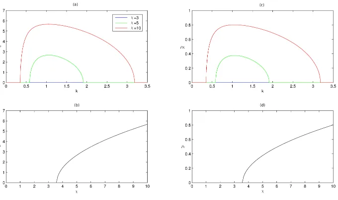
Corollary 2 - There exists a critical value for the capital-induced labor migration, ¯
χ, such that χ ≥ χ¯ implies the existence of an interval of wavenumbers (k1, k2) where
w=w(k)≤0. Besides of that, ¯χ is given by:
¯ χ=
s
1 β(1−φ) +
√
d
!2
. (18)
Note - If ρ = 0 we have thatχ ≥χ¯ is a necessary and sufficient condition for K∞ and L∞ to be unstable. That is, if there is no capital transport cost, there exists a critical value for the intensity of capital-induced labor migration, ¯χ, such that, if χ < χ, the¯ spatially homogeneous equilibrium points K∞ and L∞ are stable, and if χ ≥χ, there is¯ an interval of wavenumbers [k1, k2] where w = w(k) ≤ 0, and therefore the equilibrium
points are unstable. In terms of the original parameters, the condition for instability is give by:
χL≥b
δφ sA 11 −φ r δdL a + s dK
1−φ
!2
=:χc (19)
Now we present the main result of this paper:
Proposition 3 - Consider χ ≥ χ. Then, there exists a critical value for the capital¯ transport cost, ¯ρ, such that, if ρ≤ ρ, the spatially homogeneous equilibrium points¯ K∞ and L∞ are unstable, and if ρ >ρ, they are stable. Besides of that, this critical value is¯ given by:
¯
ρ= max
k∈[k1,k2]
r
−z
2w
v , (20)
where z,w and v are as in (17a)-(17c).
Proof - If χ > χ, by Corollary 2 we have that¯ w = w(k) ≤ 0 for some interval of wavenumbers k ∈[k1, k2], with 0< k1 < k2. Then we can write (16) as ρ≤Φ(k), where
Φ(k) is defined as Φ(k) =
q
−z2w
v , being z = z(k), w = w(k) and v = v(k) given by
(17a), (17b) and (17c), respectively. Since Φ(k) is a strictly concave function, it has an unique global maximum at some point k∗ ∈ (k
1, k2). In addition, since Φ(k) ≥ 0 ∀ k,
presents unstable modes, and the result follows
Considering the original dimensional parameters, this implies that the critical value for the physical capital transport cost is given by ρc =
q a
dKρ, provided¯ χL ≥ χc, such
as in (19). Then, if ρK ≤ρc, the spatially homogeneous equilibrium are unstable, and if
ρK > ρc, they are stable.
This is an interesting result, since it reproduces in a macroeconomic spatial growth model, a fundamental result obtained from the core-periphery model of the New Eco-nomic Geography: that there is a critical value for the transport cost above which the economy converges to a homogeneous state, and if this cost is small enough (below this critical value), the economy shows the formation of clusters (and, in the model proposed here, the development of cycles).
4
Numerical Simulations
In order to verify the spatio-temporal dynamics generated by the model and the re-sults obtained by the linear stability anasysis presented in the previous section, we will carry out numerical simulations of system (9a)-(9d). We used a standard explicit finite-difference numerical scheme in the implementation of these simulations (see Tveito and Winther (1998), for example), and considered the following parameters:
a= 0.02, b= 0.01, δ= 0.05, s= 0.2, A= 1, φ= 0.5,
which imply in the adimensional parametersβ = 2.5 andd = 1.
With these parameters, we get the critical value for the capital-induced labor migra-tion of ¯χ = 9
5 + 4
√
5 ≈3.59 (see equation (18)). Besides of that, in the simulations below
we set the size of the economy as l= 200 and consider the following initial conditions:
K(0, x) = 1, L(0, x) = 0.1e(x−100)2
49 .
In this way, we can avoid the influence of the bondary in the evolution of the initial conditions (provided we do not consider large periods of time in the simulations), since it is not possible to simulate an unbounded economy. As we comment in the conclusions, we let the analysis of a bounded economy for a future work.
physical terms, ρ.
Figure 1: Bifurcation Curves
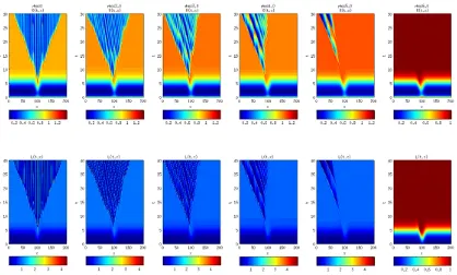
In Figure 2 we present numerical simulations showing the spatio-temporal evolution for the densities of capital (first row) and labor (second row) in the economy. In this cenario we keep the intensity of the capital-induced labor migration fixed at χ= 5>χ,¯ and vary the transport cost coefficientρ, from 0 to 3. For this χ, the critical value for the transport cost is given by ¯ρ≈2.66. Then, the spatially homogeneous equilibrium will be unstable only if ρ ≤ ρ¯≈2.66. As we can see in this figure, for ρ= 3 > ρ, the economy¯ converges to the homogeneous state of the system K∞ =L∞ = 1; for 0≤ ρ ≤ 2.5< ρ,¯ there is formation of capital and labor agglomerations. For ρ= 0, these clusters are sta-tionary and spatially symmetrical, and for 0< ρ ≤2.5 they are moving to the economy left boundary, case in which we have a break of symmetry.
In Figure 3 we show the same simulations as in Figure 2, but consideringχ= 10, case in which we will have instability only if ρ ≤ ρ¯≈ 5.67. As we can see, if ρ = 6 >ρ, the¯ economy converges to the homogeneous state; and if 0≤ρ≤5<ρ¯the economy develops unstable agglomerations and spatio-temporal cycles. Again, if ρ= 0 the economy shows spatial symmetry, but if 0< ρ≤5 all the spatial structure of the economy starts to move to the left.
5
Conclusions
In this work we introduced capital transport cost in the spatial Solow model with capital-induced labor migration considered in Juchem Neto and Claeyssen (2014). Through a linear stability analysis of the spatially homogenous equilibrium of the model (which can be easily extended for a bidimensional economy), we derived conditions for which the model enters an unstable regime where it can develop economic agglomerations and cy-cles. In particular, we derived a critical value for the transport cost such that, if the cost is smaller than this critical value, the economy may develop agglomerations and cycles (provided the capital-induced labor migration is intense enough), and if it is bigger than this critical value, the economy converges to a spatially homogeneous steady-state, with all locations having the same density of capital and labor force.
In addiction, we confirmed our linear stability analysis through numerical simulations of the model. We also observed that the introduction of a positive transport cost in the model causes a break in the symmetry of the generated spatial patterns (stable agglomer-ations and cycles), with a tendency for the agglomeragglomer-ations to concentrate in the left part of the economy. Such behavior is consistent with the hypothesis that trade only occurs in the positive x-axis direction.
In this way, with a macroeconomic model, following the approach of Regional Sciences, we reproduced a fundamental result from the core-periphery model of New Economic Ge-ography: that economic agglomerations can occur only if the transport cost is lower than a certain critical value.
Figure 2: Spatio-temporal evolution of L(t, x) and K(t, x) as a function of ρ (χ= 5)
Figure 3: Spatio-temporal evolution of L(t, x) and K(t, x) as a function of ρ(χ= 10)
References
Boucekkine, R., Camacho, C., and Fabbri, G. (2013). Spatial dynamics and convergence: the spatial ak model. Journal of Economic Theory, 148:2719–2736.
[image:12.595.90.508.372.624.2]Geographical Economics. Cambridge University Press, UK.
Brito, P. (2004). The dynamics of growth and distribution in a spatially heterogeneous world. Working Paper, ISEG, WP13/2004/DE/UECE.
Brito, P. (2005). Essays in Honour of Antonio Simoes Lopes, chapter A Spatial Solow Model with Unbounded Growth, pages 277–298. ISEG/UTL.
Camacho, C. and Zou, B. (2004). The spatial solow model. Econ. Bull., 18(2):1–11.
Camacho, C., Zou, B., and Briani, M. (2008). On the dynamics of capital accumulation across space. Eur. J. Oper. Res., (186):451–465.
Capasso, V., Engbers, R., and La Torre, D. (2010). On a spatial solow model with techno-logical diffusion and nonconcave production function. Nonlinear Anal-Real, (11):3858– 3876.
Capasso, V., Engbers, R., and La Torre, D. (2012). Population dynamics in a spatial Solow model with a convex-concave production function, pages 61–68. Mathematical and Statistical Methods for Actuarial Sciences and Finance. Springer-Verlag, Milano, Italy.
Combes, P.-P., Mayer, T., and Thisse, J.-F. (2008). Economic Geography - The Integra-tion of Regions and NaIntegra-tions. Princenton University Press, UK.
Edelstein-Keshet, L. (2005). Mathematical Models in Biology. Classics in Applied Math-ematics. SIAM, Philadelphia, US.
Engbers, R. (2009). Spatial Structures in Geographical Economics - Mathematical Model-ing, Simulation and Inverse Problems. PhD thesis, Westfalische Wilhems-Universitat, Munster.
Fujita, M., Krugman, P., and Venables, A. J. (1999). The Spatial Economy. MIT Press.
Fujita, M. and Thisse, J.-F. (2002). Economics of Agglomeration: Cities, Industrial Location, and Regional Growth. Cambridge University Press, UK.
Isard, W. (1956).Location and Space Economy: A General Theory Relationg to Industrial Location, Market Areas, Land Use, Trade and Urban Structure.MIT Press, Cambridge.
Isard, W. (2003). History of Regional Science and the Regional Science Association International - The Beginnings and Early History. Spring-Verlag, Berlin.
Isard, W. and Liossatos, P. (1975a). Parallels from physics for space-time development models: Part i. Reg Sci Urban Econ, 1(1):5–40.
Isard, W. and Liossatos, P. (1975b). Parallels from physics for space-time development models: Part ii - interpretation and extensions of the basic model. Regional Science Association, 35:43–66.
Juchem Neto, J. P. and Claeyssen, J. C. R. (2014). Capital-induced labor migration in a spatial solow model. Journal of Economics, 112(2):1–23.
Krugman, P. (1979). Increasing returns, monopolistic competition and international trade. Journal of International Economics, 9:469–479.
Krugman, P. (1991). Increasing returns and economic geography. J Polit Econ, (99):483– 499.
Murray, J. D. (2003). Mathematical Biology - II: Spatial Models and Biomedical Appli-cations. Springer-Verlag, New York, US, third edition edition.
Quigley, J. M. (2001). The renaissance in regional research. The Annals of Regional Science, 35:167–178.
Tveito, A. and Winther, R. (1998). Introduction to Partial Differential Equations - A Computational Approach. Springer-Verlag, New York. 11. Reaction-Diffusion Equa-tions: pp. 337-360.