Career Mobility Patterns of Public
School Teachers
Vera, Celia Patricia
Zirve University
23 August 2013
Teachers
Celia P. Vera∗
Zirve University
August 2013
Abstract.-One issue that has pervaded policy discussions for decades is the difficulty that school districts experience in retaining teachers. Almost a quar-ter of enquar-tering public school teachers leave teaching within the first three years and empirical evidence has related high attrition rates of beginner teachers to family circumstances, such as maternity or marriage. I examine female teach-ers’ career choices and inquire about the effects that wage increases and child care subsidies have on their employment decisions. I set up a dynamic model of job search where individuals simultaneously make employment and fertility decisions, fit it to data from a national longitudinal survey and estimate it by Simulated Method of Moments. Estimates indicate that gains of exiting the teaching workforce to start a family vary between 75% and 88% of the average teaching wage if the exit occurs during the first five years. At late periods and provided a positive stock of children, nonpecuniary penalties to return to teach lie between one and two times the average teaching wage. A 20 percent raise in teaching wages increases retention by 14% and decreases the proportion of teachers giving birth by 50%. Results suggest that fertility changes occur not only at earlier periods but also after a career interruption when teachers are considering a returning decision. The effectiveness of the wage policy in attracting back to the field individuals who left teaching to enroll in nonteaching jobs is positively associated with the greatest impact that the policy has on fertility in nonteaching. Child care subsidies increase retention by 11% and 29% with the lowest and highest subsidy, respectively. New births are concentrated at earlier periods of teachers’ careers and thus, generate longer first teaching spells. However, large nonpecuniary rewards at late periods of the non labor market alternative relative to being in teaching as well as exits out of the workforce concentrated at later periods lead the decrease of returning rates of teachers who dropped the workforce altogether.
Keywords: Teachers, Fertility, Attrition, Structural Model.
JEL Classification: J13, J44, J45, C61.
∗Email address: celia.vera@zirve.edu.tr. I am grateful to Silvio Rendon, Hugo
1
Introduction
One particular issue that has pervaded policy discussions for decades is the difficulty that
school districts experience in retaining teachers. Almost a quarter of entering public school
teachers leave teaching within the first three years (Keigher, 2010). Empirical evidence has
related high attrition rates of beginner teachers to family circumstances, such as maternity
and marriage.1 This is consistent with the reality that women account for approximately
76% of the national public teaching force (NCES, 2012) and that teachers can reentry the
sector after a career interruption without suffering a wage loss.2 These demographic and
institutional features have two important implications. First, the option of leaving the
workforce may be especially appealing for those in the teaching occupation. Second, family
size variables acquire an influential role in determining employment decisions. As stated by
Flyer and Rosen (1997), Stinebrickner (1998, 2001a,b, 2002) and Stinebrickner et al. (2006),
those with a bigger taste for spending time with their children are not only more likely to
leave the workforce when they start a family, but also to select teaching as a profession.
Despite it is well established that family formation variables play an important role in
ex-plaining teachers’ career choices, there is no study that jointly models teachers’ labor market
and fertility decisions. In this paper, I fill this gap by specifying and estimating a dynamic
model of individual decision-making that endogenously accounts for fertility and that is
con-ducive for simulating the effects that potential wage changes and child care subsidies would
have on female teachers’ employment decisions. By allowing fertility and labor supply be
jointly determined, the model considers an extra effect on labor supply that previous studies
did not take into account. The additional effect comes from the impact of both policies on
fertility choices, which in turn affects labor-force attachment to the teaching sector. I find
that wage policies have a negative effect on fertility, and thus increase retention through
lower attrition rates and higher returning rates. On the other hand, child care subsidies
1
In this paper, I refer to attrition as voluntary separations from the entire public school system. While movements of teachers across schools or districts represent attrition from individual schools or districts, it does not correspond to teachers leaving the teaching profession entirely. Similarly, most attrition from teach-ing is voluntary given widespread tenure rates and the prevalence of unionized grievance policies regardteach-ing termination.
2
have a positive effect on fertility and increase the first teaching spell as more births occur at
earlier periods of their careers.
Another way the present paper differs from previous works is that it offers a different
approach to understand teachers’ retention. While most efforts have been focused on
exam-ining the length of the first teaching spell, I think of retention as a joint outcome of attrition
and returning decisions.3 Therefore, through this paper, I quantify the impact of regime
changes on both attrition and returning rates. My results show that the effectiveness of
higher wages in attracting former teachers who left teaching to enroll in nonteaching jobs
responds to the greatest impact that this policy has in reducing births in the nonteaching
sector. On the other hand, child care subsidies yield longer first teaching spells, especially for
those who dropped the workforce entirely. Although attrition rates focused at later periods
partially explain why fewer returners are observed,4 results suggest that large nonpecuniary
rewards outside the workforce relative to being in teaching keep teachers away from public
schools at later periods.
The impending shortfall of teachers that attrition creates would force many of the
na-tion’s school systems to lower standards to fill the increasing number of teaching openings,
inevitably resulting in a less qualified teaching force and lower school performance. Teacher
attrition may affect student learning in several ways. First, in high-turnover schools, students
may be more likely to have inexperienced teachers who are less effective on average (Rockoff,
2004; Rivkin et al., 2005; Kane et al., 2006). Second, high turnover creates instability in
schools, making it more difficult to have coherent instruction.5 Third, high turnover can be
costly in that time and effort is needed to continuously recruit teachers.
In an attempt to quantify attrition costs, Milanowski and Odden (2004) signal that every
time a school district loses an experienced teacher with two or more years of experience and
is forced to hire a novice teacher, the students assigned to the novice teacher over the first
two years of their career lose roughly 0.10 standard deviation in student achievement. Based
on this result and using the estimations of the value of a one standard deviation gain in math
3
Given that institutional arrangements facilitate reentry to the sector, whether certified teachers will be adequate depends on both the length of time that new entrants stay in the classroom and the percentage of teachers who return to teaching after a career interruption.
4
Longer first teaching spells reduce the likelihood of former teachers to be observed back to the field.
5
that Kane and Staiger (2002) present in their work, Staiger and Rockoff (2010) conclude that
the monetary value of the loss in student achievement outweighs the direct hiring costs.
Not only are teachers central to promoting student achievements, but their compensation
represents an important portion of the national investment in public education. According
to the work by Speakman et al. (1996) and Guthrie and Rothstein (1999), in a typical school
district, wages account for at least half of the expenditures.
Previous research has established that a strong, positive relationship exists between
teacher pay and the length of time that a person remains in his/her first teaching job.6
Although some studies suggest that child care provision may have significant positive effects
on retention, potential initiatives have not been empirically tested. Stinebrickner’s (2001b)
estimates indicate that this would not be a cost-effective policy given the large effect that
children have on nonpecuniary utility of teachers. According to his estimates, a female
teacher with a single child would have to receive a pay rise of approximately 60 percent to
keep her utility from teaching relative to not working, the same as it would be if she had
no children. Frijters et al. (2004) and Stinebrickner et al. (2006) also mention a day care
subsidy for women with young children as a policy alternative but rely on Stinebrickner’s
(2001b) results to conclude that this may not be a cost-effective policy.
Relatively few studies have examined former teachers’ reentrance into the public school
workforce. Those that have analyzed the issue have used “teacher-specific” data that were
constructed from administrative records of a particular state or school district and, as a
result, contained no information about the labor force status of individuals after they left
teaching, or family formation variables.7 Murnane et al. (1988) found that the percentage
of Michigan returner teachers varies from 28% to 31% and is higher for younger women.
Kirby et al. (1991) reported returning rates for teachers in Indiana of 30% of new hires.
Using data for the state of Michigan, Beaudin (1993) found that teachers with subjects area
specialties that provide limited opportunities for better paying employment outside of public
schools, teachers who have more than two years of experience and a master’s degree, and
6
See Murnane and Olsen (1989, 1990),Gritz and Theobald (1996), Stinebrickner (1998) and Dolton and van der Klaauw (1999) for an examination of the issue in reduced-form models and van der Klaauw (2012), Stinebrickner (1998, 2001a,b) for an overview of teacher attrition in a dynamic setting.
7
those who interrupted their careers at an older rather than at younger age are more likely
to return. Grissmer and Kirby (1997) performed a descriptive analysis of National Center
for Education Statistics data and found that during the 1980s returning teachers composed
about 40 percent of all entering teachers.
I construct a dynamic model where individuals jointly make employment and fertility
decisions. Data on wages, employment and fertility choices allow the model to separately
identify how wages and nonpecuniary utility in the various options affect labor market
de-cisions. With this framework, I generate predicted life-cycle trajectories and distributions
for employment status, wages, and fertility that match the observed ones. The behavioral
parameters of the model are recovered through the Simulated Method of Moments using
data from a general longitudinal survey of high school graduates.
The remainder of this paper is set out as follows. Section 2 introduces the data and
describes the salient characteristics of the sample. The model and estimation methodology
are outlined in sections 3 and 4 with a discussion of the estimation results being provided in
section 5. Section 6 evidences the model fit. Section 7 simulates the two policy experiments
and section 8 concludes.
2
Data
The data come from the National Longitudinal Study of the High School Class of 1972
(NLS-72). This survey collects longitudinal data on post-secondary educational activities of
a sample of high school seniors who graduated in 1972. The first wave was completed in
1972. Follow up surveys were taken in 1973, 1974, 1976, 1979 and 1986. For each person the
survey contains detailed information about work experience, education, marriage and fertility
decisions. Individuals who had teaching experience or were certified to teach in elementary
or secondary schools were sent a Teaching Supplement questionnaire which asked questions
about their teaching experiences. This specific questionnaire applied to teachers has been
relevant to identify the final sample and to construct job and personal histories. Given that
teachers were oversampled in the survey design, the NLS-72 provides a valuable source for
the study of teachers’ mobility patterns.
respond different than females to family formation variables,8 the final sample consists of
391 female teachers.9
Since this paper focuses on career choices after certification and most individuals spent
four years after high school in training courses to be certified, the final data set contains
between one and eleven years of information for every individual. Most individuals are
observed ten or fewer years, only those who spent three years in college are observed eleven
years.
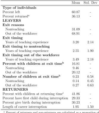
Table 1 presents descriptive statistics of the final sample and indicators of exits and
returns.10The proportion of female teachers with a break in their careers is 61% and the main
exit reason is to drop the workforce altogether (69% of leavers drop the workforce altogether
and the remaining 31% leave her teaching job to work in the nonteaching sector).11
On average, a career interruption occurs after 3.20 years of teaching experience. The
length of time becomes 2.55 years if the exit reason is to enroll in the nonteaching sector,
and 3.49 years if the exit reason is to drop the workforce altogether. Regarding family-size
variables, 17% of teachers who leave the field have at least one child at exiting time. The
percentage of departing teachers with children at exiting time is 9% and 20% for exits to
nonteaching and out of the workforce, respectively.
Table 1 shows that 36% of departing teachers return at some point to a teaching job.12
Returner teachers stay out of teaching in average 1.95 years and 30% of them give birth to
new children at least once during career interruption. At returning time, 42% of them have
at least one child.
8
Stinebrickner (2001a) found that whereas the participation rate in nonteaching occupations remains largely unchanged for the female sample between the years when the teaching participation declines, it increases significantly for the male sample, suggesting that a large increase in the proportion of women who are out of the workforce plays a more important role in their declining teaching participation rate whereas the large increase in male teachers who start a nonteaching job explains the decrease in the male teaching participation rate.
9
The sample of teachers was constructed in the following way: among the 750 individuals who responded all waves and the Teaching Supplement, who became certified to teach and who said in the Teaching Supple-ment they have had some teaching experience, 137 were dropped because they had some missing data which made impossible to construct work and personal histories. From the remaining, 82 records were dropped because they did not have teaching experience after certification. 73.63% of the remaining sample are female. Therefore, the final sample consist of 391 female teachers.
10
People are considered to be“working” if they work more than 20 hours a week. Thus, the “out of the workforce” designation includes individuals who are working fewer than 20 hours a week.
11
The exit reason is determined by the person’s activity in the period after departure.
12
3
The Dynamic Model
Each individual has a finite decision horizon beginning the year after they get certified and
exogenously ending 40 periods later. At the beginning of each school year, a particular
female teacher seeks to maximize her expected lifetime utility by choosing (i) an exclusive
employment alternative, jt = 0 (not to work),131 (to work in a teaching job), or 2 (to work
in a nonteaching job) and (ii) whether she has a child (bt= 1) or not (bt= 0). Let d denote
the available alternatives: d = 1 if she has a teaching job and doesn’t give birth; d = 2 if
she has a teaching job and gives birth; d = 3 if she has a nonteaching job and doesn’t give
birth; d= 4 if she has a nonteaching job and gives birth,d= 5 if she is out of the workforce
and doesn’t give birth, and d= 6 if she is out of the workforce and gives birth.
The law of motion for the number of children is:
kt+1 = kt+bt if 0≤kt≤2 and,
= 3 if kt = 3, (1)
where kt represents the number of children at the beginning of period t. Equation (1)
captures the idea that the maximum number of children allowed in the model is three.
Therefore, the number of mutually exclusive alternatives from which she can choose every
period depends on the stock of children at the beginning of every period. If kt < 3, she
can choose from alternatives d = 1,2,3,4,5,6 whereas if kt = 3, she can only choose from
alternatives d= 2,4,6.
The set of available employment options in a given year depends on the person’s
employ-ment status in the previous year. If int−1 the individual is employed as a teacher, in t she
has the option of returning to the previously held job and also receives a new nonteaching
job offer drawn from a wage offer distribution FN(.),(xN ∈ (ωN, ωN),0 < ωN < ωN <∞).
Likewise, if in t−1 the person is employed in a nonteaching job, in t she has the option of
returning to the previously held job and also receives a new teaching job offer drawn from
a different wage offer distribution FE(.)(xE ∈(ωE, ωE),0< ωE < ωE <∞). If in t−1 the
person is out of the workforce, in t she receives a teaching job offer with probability ρ and
13
a non teaching job offer with probability 1−ρ, both job offers are drawn from wage offer
distributions FE(.) and FN(.), respectively. The person has always the option of choosing
the non labor market alternative.
The utility teachers derive from their choices each period contains pecuniary and
non-pecuniary benefits. The first component, non-pecuniary utility, equals her wage income. The
second component, nonpecuniary utility, has an occupation-specific part and a
children-specific part. The former nonpecuniary part comes from all the nonpecuniary enjoyment
and dislikes that the teacher receives from a specific occupation and is activated only when
the teacher is working (either teaching or nonteaching). The children-specific part has a
similar interpretation and is activated only if the teacher has children for all employment
al-ternatives. Stochastic changes in the utility of each choice are captured by random variation
in her wage earnings.
Let Wr
t and Qrt represent the pecuniary and nonpecuniary utility (in wage equivalents),
respectively, that a particular teacher receives at time tfrom employment alternativer. Let
r = E, r =N, and r = H denote a teaching job, a nonteaching job, and the home option,
respectively. The total current period utility Ur
t that a particular teacher receives in t by
choosing employment sector r is assumed to be additive in Wr
t and Qrt:
Utr =Wtr+Qrt, for r=E,N,H.
The pecuniary utility is given by:14
Wtr = ωrEXP(α1r t+αr2t2) for r=E,N and
WtH = 0.
The nonpecuniary utility is given by:
Qrt =γr+α3r kt+αr4ktt+αr5ktt2 +αr6 k2t +α r
7 k2t t+α r
8kt2t
2, for r=E,N,H. (2)
The first term in equation (2), γr, is the occupation-specific part and represents the
nonpecuniary utility in teaching and nonteaching jobs relative to the nonpecuniary utility
14
derived from not working when the teacher doesn’t have children.15 The remaining terms
represent the children-specific part and are assumed to be quadratic to reflect diminishing
returns of children. Functional forms of pecuniary and nonpecuniary utilities imply that if
the teacher is not working she will not receive any wage income nor nonpecuniary utility
unless she has children.
In this model, rather than being myopic, the teacher knows that current period decisions
affect future utility through the determination of her available options in the future. The
setting up of this model is closely related to the way teaching markets work. The teacher
knows that one result of choosing to teach in the current period is that she will accumulate
an additional year of teaching experience. Given the rigidity in the teaching wage structure,
the extra year of experience is likely to have an important effect on future teaching wages.
Therefore, a set up in which the individual cares not only about her current period utility but
also about the discounted utility that she will receive over a finite work horizon is needed.
A dynamic model performs this task.
However, although the teacher is assumed to know with certainty the utility associated
with each option in the current period, this is not accurate about future periods; in reality,
the teacher cannot know exactly what types of jobs (wages and nonpecuniary characteristics)
will be offered to her in the future. For instance, she knows that if she currently is employed
in a teaching job, she can hold the job next period but she is uncertain about the value of
the nonteaching wage offer she will receive. This is how the model captures uncertainty:
the future realizations are not known (although the individual does know the distributions)
which implies that, for an optiond, the teacher can not compute the exact discounted utility
that she will receive over her finite work horizon but, instead, calculates and makes decisions
based on the discounted expected utility of the option over her finite work horizon.
A teachers’ expected present value of lifetime rewards depends on her employment status
the previous period and on how many children she enters the current period with.16
Partic-ularly, if in period t−1 she is employed in a teaching job withωE and has accumulatedk
t−1
15
This is a result of normalizingγH
to zero.
16
The number of children a teacher enters periodt with, kt, is equivalent to the stock of children
children, her expected lifetime utility in t is:
VE(kt, ωE, t) = UtE +βEmax [V E(k
t, ωE, t+ 1), VE(kt+ 1, ωE, t+ 1),
VN(kt, ωN, t+ 1), VN(kt+ 1, ωN, t+ 1),
VH(kt, t+ 1), VH(kt+ 1, t+ 1)]. (3)
= UtE +β
Z
max [VE(kt, ωE, t+ 1), VE(kt+ 1, ωE, t+ 1),
VN(kt, xN, t+ 1), VN(kt+ 1, xN, t+ 1), VH(kt, t+ 1),
VH(kt+ 1, t+ 1)]dFN(xN), if kt<3.
and
VE(kt, ωE, t) = UtE +βEmax [V E
(3, ωE, t+ 1), VN(3, ωN, t+ 1), VH(3, t+ 1)].
= UtE +β
Z
max [VE(3, ωE, t+ 1), VN(3, xN, t+ 1),
VH(3, t+ 1)]dFN(xN), if kt= 3.
expected lifetime utility depends on how many children she enters t with. It is given by:
VN(kt, ωN, t) = UtN +βEmax [V E(k
t, ωE, t+ 1), VE(kt+ 1, ωE, t+ 1),
VN(kt, ωN, t+ 1), VN(kt+ 1, ωN, t+ 1),
VH(kt, t+ 1), VH(kt+ 1, t+ 1)] (4)
= UtN +β
Z
max [VE(kt, xE, t+ 1), VE(kt+ 1, xE, t+ 1),
VN(kt, ωN, t+ 1), VN(kt+ 1, ωN, t+ 1), VH(kt, t+ 1),
VH(kt+ 1, t+ 1)]dFE(xE), if kt<3
and
VN(kt, ωN, t) = Ut+βEmax [VE(3, ωE, t+ 1), VN(3, ωN, t+ 1), VH(3, t+ 1)]
= UtN +β
Z
max [VE(3, xE, t+ 1), VN(3, ωN, t+ 1),
VH(3, t+ 1)]dFE(xE), if kt = 3.
depends on the stock of children accumulated in t−1, and it is :
VH(kt, t) = UtH +β {ρEmax [V E(k
t, ωE, t+ 1), VE(kt+ 1, ωE, t+ 1),
VH(kt, t+ 1), VH(kt+ 1, t+ 1)] +
+(1−ρ)Emax [VN(kt, ωN, t+ 1), VN(kt+ 1, ωN, t+ 1),
VH(kt, t+ 1), VH(kt+ 1, t+ 1)]}. (5)
= UtH +β {ρ
Z
max [VE(kt, xE, t+ 1), VE(kt+ 1, xE, t+ 1),
VH(kt, t+ 1), VH(kt+ 1, t+ 1)]dFE(xE) +
(1−ρ)
Z
max [VN(kt, xN, t+ 1), VN(kt+ 1, xN, t+ 1),
VH(kt, t+ 1), VH(kt+ 1, t+ 1)]dFN(xN)}, if kt <3.
and
VH(kt, t) = UtH +β {ρEmax [VtE(3, ωE, t+ 1), VH(3, t+ 1)] + +(1−ρ)Emax [VtN(3, ωN, t+ 1), VH(3, t+ 1)]}.
= UtH +β {ρ
Z
max [VE(3, xE, t+ 1), VH(3, t+ 1)]dFE(xE) +
+(1−ρ)
Z
max [VN(3, xN, t+ 1), VH(3, t+ 1)]dFN(xN)}, if kt = 3.
Notice that the pair of employment alternatives inside the expectation term in
equa-tions (3) to (5) correspond to the opequa-tions of giving birth or not. Therefore, kt+1 has been
expressed in terms of kt, as equation (1) indicates.
Agents solve the dynamic problem with a finite horizon T=40. Given the sample period
in the data, I generate life cycle choices of employment and fertility for 11 periods.
4
Estimation Methodology
The estimation strategy is a Simulated Method of Moments procedure and its aim is to
parame-ter set, I solve the Dynamic Programming problem, generate simulated paths of
employ-ment and fertility, and construct a criterion function that measures the distance between
the observed and simulated moments. I minimize the criterion function and find the
pa-rameter estimates of the theoretical model, φ = {Θr, αH
3 , αH4 , αH5 , α6H, αH7 , αH8 , ρ} where Θr={γr, αr
1, αr2, αr3, α4r, αr5, αr6, αr7, αr8, µr, σr} for r=E,N. The criterion function is as follows :
S(φ) = 12
X
j=1
Nj X
i=1
W Tij(Rijobs−R sim ij )
2,
where N1 = 33 are the employment status (3 moments × 11 years), N2 = 44 are the wage
levels (4 moments × 11 years), N3 = 44 are the children status (4 moments × 11 years),
N4 = 30 are the employment transitions from teaching (3 moments × 10 years), N5 = 30
are the employment transitions from nonteaching (3 moments× 10 years), N6 = 30 are the
employment transitions from out of the workforce (3 moments × 10 years), N7 = 20 are
the number of children transitions from no children (2 moments × 10 years), N8 = 20 are
the number of children transitions from one child (2 moments × 10 years), N9 = 20 are the
number of children transitions from two children (2 moments×10 years), N10= 110 are the
attrition rates (11 moments× 10 years),N11 = 20 are the returning rates from nonteaching
(2 moments × 10 years), N12 = 20 are the returning rates from out of the workforce (2
moments × 10 years), and W T is a weighting matrix. In this study, W T is an identity
matrix and each moment is weighted the same.
Thus, there are 322 moments to estimate 29 parameters. I use the model to simulate
employment, wages and fertility choices at every period.17 The function is minimized using
Powells method (Powell, 1964), which require function evaluations but not derivatives.
5
Estimation Results
The parameters that characterize the pecuniary utility are reported in the upper part of
Table 2. Teaching jobs present a higher mean and a lower standard deviation of the
log-wage offer distribution than nonteaching jobs. These parameters imply an estimated initial
17
mean yearly wage offer for teaching jobs of $10,482.75 and of $9,477.11 for nonteaching jobs.
The wage growth parameters show that wages grow at a declining rate for both teaching
and nonteaching occupations.
The estimated parameters of the nonpecuniary utility are reported at the middle of
Table 2. The nonpecuniary constant is negative for both teaching and nonteaching jobs
reflecting the fact that teachers perceive a negative satisfaction when they are working
rela-tive to the leisure option. The nonpecuniary constant is less negarela-tive for teaching than for
nonteaching jobs, suggesting that teachers find more enjoyable (or less unpleasant) working
in a teaching job than in a nonteaching job.
The parameters related to the number of children provide information of the effect that
children have on teachers’ nonpecuniary utility. An intuitive way to explain the employment
flows across teachers’ careers is analyzing choice premia of several alternatives. I present
below a discussion of three different premia calculated. They are expressed in terms of the
average teaching wage to facilitate economic interpretation.
The “children premia” correspond to the nonpecuniary rewards of having children given
a particular employment sector.18 They measure the gains of starting and enlarging families
in a particular occupation. Table 3 displays children premia for the first, second and third
birth. The marginal nonpecuniary utility of the first child is only positive if the teacher
is employed in a nonteaching job or if she is out of the workforce, and it is greater in the
latter case. For instance, the nonpecuniary gain of having the first child in the nonteaching
sector in year 5 is equivalent to 3% of the average teaching wage, whereas it corresponds to
12% if she is out of the workforce. The loss of starting and enlarging families during the
first five years doesn’t exceed 2 percent of the teaching wage but becomes important at late
periods.19 This suggests that if the individual is employed in a teaching job, she does not
have nonpecuniary incentives to give birth to her first child and keep her current teaching
job. An interesting result is that the well established diminishing returns on having children
only hold for the nonteaching and home options.20 As a result, the teaching sector is the
only employment option generating rewards to give birth to a third child after period five.
18
It has been calculated asQr
t(k+ 1)−Q r
t(k), forr=E, N, H andk= 0,1,2. 19
If the first birth occurs in period 12, the loss is equivalent to 19 percent of the teaching wage.
20
The “occupation premia” evaluate the nonpecuniary gains of employment alternatives
conditional on a positive stock of children.21 These premia are important to identify gains
and losses of reentry teaching with children after a career interruption. Table 4 shows that
provided a positive stock of children, a reentry to teaching is only rewarding if the former
teacher returns from the nonteaching sector. For instance, the gain of doing so during
periods 8-12 varies between 61 and 47 percent of the average teaching wage, whereas the
nonpecuniary penalty of reenter teaching from out of the workforce in the same period lies
between 1.24 and 1.96 times the average teaching wage. The gain (loss) decreases (increases)
with time suggesting that rewards of returning to teach with children are more important
at early years when children are younger.
Table 4 also indicates that given a positive number of children, the non labor market
al-ternative offers nonpecuniary rewards relative to both teaching and nonteaching employment
sectors.22 Conditional on having two children, choosing a teaching job instead of staying out
of the workforce in year 5 is equivalent to a loss of 91% of the average current teaching wage,
whereas being enrolled in a nonteaching job rather than not working at all has a
nonpecu-niary loss equivalent to 1.59 times the teaching wage in the same period. The fact that being
in nonteaching generates a greater loss than being in teaching complements our
understand-ing of the negative values of γE and γN shown in Table 2. These results suggest that both
with and without children, working in teaching is always better than being employed in a
nonteaching job.
The “children cross premia” evaluate the nonpecuniary gains of giving birth in the current
employment, as well as the gains of switching employment sectors to do so, and thus are
relevant to understand exit behavior.23 Tables 5 and 6 show that regardless of the stock of
children, it is rewarding to exit the workforce to give birth. The gain is greater if individuals
21
The nonpecuniary gain of teaching relative to nonteaching has been calculated as QE
t(k)−Q N t (k),
for k = 1,2,3; the nonpecuniary gain of teaching relative to out of the workforce has been calculated as
QE
t(k)−Q H
t (k), fork = 1,2,3; the nonpecuniary gain of nonteaching relative to out of the workforce has
been calculated asQN
t (k)−Q H
t (k), fork= 1,2,3. 22
Recall that the teaching-out of the workforce premium is equivalent to the negative of the out of the workforce-teaching premium. Therefore, the negative values of the premia shown in Figures 5.2(b) and 5.2(c) imply a positive value for the out of the workforce-teaching premium.
23
The teaching cross premium has been calculated subtractingQE
t(k) fromQ r
t(k+ 1), fork= 0,1,2 and
r = E, N, H; the nonteaching cross premium has been calculated subtracting QN
t (k) from Q r
t(k+ 1), for
k= 0,1,2 andr=E, N, H; and the out of the workforce cross premium is the subtraction ofQHt (k) from
Qr
drop the workforce from nonteaching rather than from teaching, reinforcing the
“family-friendly” characteristic usually attributed to the teaching occupation. Nonpecuniary benefits
of dropping out the workforce to give birth to the first child during the first five years lie
between 75 and 78 percent of the average teaching wage if the exit is from the teaching
sector, and vary between 1.45 and 1.59 times the teaching wage if the departure is from the
nonteaching option. Also, the law of diminishing returns only holds for the nonteaching and
home sector. The gain in exiting the teaching workforce increases with time and the number
of children until the second birth. For instance, the nonpecuniary gain of giving birth to a
first child in the non labor market alternative relative to teaching in year 5 is equivalent to
88% of the average teaching wage. The gain becomes 90% and 82% of the teaching wage if
the birth corresponds to the second and third child, respectively.
These trends are supported by the out of the workforce cross premium presented in
Table 7. The non labor market alternative offers nonpecuniary gains of giving birth to the
first two children relative to both teaching and nonteaching sectors. A third birth produces
nonpecuniary losses in all employment sectors relative to the non labor market alternative.
The loss is greater if the third birth occurs in the nonteaching sector, which supports the view
that the nonteaching sector is the least rewarding employment alternative to have children.
Although the lifetime expected utility, represented by the value function, considers the
expected utility of future periods besides the instantaneous utility, the previous analysis
provides an idea of the forces that drive teachers’ decisions. The model predicts that as
families are created or enlarged, female teachers become relatively less likely to be employed
in teaching jobs and become more likely to drop the workforce altogether.24 At late periods,
when families have been created, the non labor market alternative offers large nonpecuniary
rewards relative to teaching. The nonpecuniary losses of returning with children to the
teaching sector between years 8-12 lie between one and two times the average teaching wage.
24
6
Model Fit
To assess how well the parameter estimates mimic the data, I compare the observed and the
predicted choice distributions and transitions of the moments specified in Section 4.
Table 8 compares actual and predicted employment and wage moments for selected years.
The observed teaching decreasing trend is very well fit by the model prediction. However,
the model barely replicates the flow occurring in reality between teaching and the non
la-bor market alternative at earlier years, probably as a result of an over prediction of the
nonteaching wage which in turn drives more individuals to the nonteaching sector.
Since the analysis time in this paper is years after certification, transitions shown in
Table 8 reproduce how teachers move across employment options and do not necessarily
represent exit and return rates.25 The model is able to replicate occupation flows closely,
especially transitions from out of the workforce, which although not perfectly, are related to
the reentry into the teaching sector. However, predicted transitions to out of the workforce
from teaching and nonteaching sectors do not exhibit the same pattern at early years of their
observed counterpart. This may be related to the underestimation of the predicted share of
individuals in the non labor market alternative at early years discussed above.
Table 9 displays actual and predicted number of children distributions. The replication
of these moments is fairly good. The predicted zero percentage of individuals who give birth
to a third child is a result of the low or negative premium that a third birth generates, as
discussed in Section 5.
Predicted and actual return rates are reported in Table 10.26 The model is very accurate
to replicate returning rates if the exit reason has been to drop the workforce. The returning
rates for exits to the nonteaching sector are slightly understated, specially for individuals
who are observed few years after departure. The ability of the model in better replicating
25
For instance, an individual who started her teaching spell at the beginning years after certification, who left after few years and never came back to teach is included in the group of non returners, as well as the individual who started her teaching spell many years after certification, left one or two years before the end of survey and was never seen again in the survey. However, given that both individuals have their first teaching spells at different times during their career paths, it is very likely that the second individual comes back to teach after the last year of observation in the survey which would make her belong to a different group if the data contained more years of observation.
26
returning rates for exits out of the workforce reinforce the overall fit of my estimates since
the model is particularly successful in reproducing reentry decisions for departing teachers
who exited for family circumstances. This in turn indicates that the proposed model is able
to identify that family formation variables matter not only at exiting but also at returning
time.
7
Policy Experiments
After recovering the behavioral parameters and assessing their success in replicating the
data, I explore the effects of two regime changes on teachers’ career choices. First, I consider
raising the salary of all teachers by 20 percent. This uniform wage increase, which will
be referred to as “policy one” represents an increase in the pecuniary benefits of choosing
a teaching job and is consistent with the current rigid wage structure in public schools.
Second, to illustrate the link between teachers’ employment decisions and family changes, I
increase the children-specific component of the nonpecuniary teaching utility. This policy,
referred to as “policy two” can be viewed as a child care subsidy if we consider that it also
represents the net benefit of having children.27 I have simulated the effects of three different
amounts and I will refer to them as subsidy “level i,” where i= 1,2,3 and higher values of
i represent larger subsidies.28
7.1
Policy One: A 20 Percent Increase in Teaching Wages
Figure 1 compares predicted and counterfactuals participation rates, wages and children
distributions for policy one. Higher teaching salaries increase the teaching participation
rate from period 3 and the effect becomes more significant with time. At period three, the
proportion of teachers employed in teaching jobs increases by 1.3%; at period seven, the
increase is by 18% and at the last period, the effect is 20%. Figures 1c and 1d suggest that
a large decrease in the proportion of women who are out of the workforce, rather than more
27
Implementing a child care subsidy is equivalent to increasing the net benefit of having children and being employed in a teaching job (which will reduce the cost of having children). In terms of the model, policy two has been implemented by modifyingαE
3. 28
The equivalent in dollars for every subsidy level as well as the corresponding change in the children parameter,αE
individuals leaving nonteaching jobs, plays the relevant role in this trend.
The measure of retention used in this paper is the percentage of aggregate years spent
in teaching.29 A 20 percent raise in teaching pay increases retention by 14% (from 66%
to 75%).30 Consistent with the previous analysis, the higher retention responds to a larger
decrease in the aggregate years spent out of the workforce rather than to a decline in the
proportion of years spent in nonteaching.31
Figure 1d is illustrative of changes in fertility choices. Over my sample period, the
proportion of teachers without children increases from 68% to 82%.32 A closer examination
to the data indicates that this result is mainly attributed to fertility changes occurring in
the nonteaching sector. The average birth rate for teachers employed in nonteaching jobs
decreases by 21% whereas it declines by 7% for individuals out of the workforce and remains
constant in the teaching sector.33
Taking employment and fertility changes together, results suggest that teachers perceive
working in a teaching job and having children as exclusive goods and that they find rewarding
to be employed in a teaching job only if they have fewer children.
Columns one and two of Tables 12 and 13 compare attrition rates of the benchmark
model and policy one for exits to nonteaching jobs and out of the workforce, respectively.
The discussion of attrition is accompanied by an analysis of indicator of exits and returns
presented in Table 14. According to Table 14, higher teaching wages diminish the percentage
of teachers leaving the field from 56% to 43% and the average length of the first teaching
spell from 3.94 to 3.61 years. The effect on the stay in teaching is greater if the exit reason is
to drop the workforce altogether.34 The first columns of Tables 12 and 13 show that attrition
rates are lower at every period, regardless of their destination sector.
The bottom part of Table 14 depicts fertility behavior of teachers at exiting and returning
29
Stinebrickner (2001a,b) also uses the same indicator.
30
Importantly, this may underestimate the effect of the relative wage hike on the stock of public school teachers as there may be a further beneficial effect on recruitment.
31
The aggregate years spent in nonteaching decrease by 15% whereas the aggregate years spent out of the workforce decline by 50%.
32
This proportion has been calculated as the weighted average of the percentage of teachers without children at every period.
33
The model predicts that no birth to new children occurs in the teaching sector and policy one does not change this pattern.
34
times. Whereas 50% of returners have at least one child at returning time in benchmark, this
percentage decreases to 25% with policy one, suggesting that changes in fertility behavior
occur not only at early periods as more teachers are employed in teaching jobs, but also
after a career interruption when they are considering to return. The 53% decrease in the
proportion of returners who give birth to new children at least once during career interruption
confirms this view.
To understand reentry behavior, I present return indicators in Table 14 and compare
returning rates for exits to nonteaching and out of the workforce under benchmark and
policy one in columns one and two of Tables 15 and 16, respectively. Table 14 shows that
the proportion of teachers who return to the field after a career break increases from 32% to
48% and that the length of time out of teaching doesn’t change significantly. According to
Tables 15 and 16, returning rates for teachers observed different periods after leaving increase
regardless of the exit destination sector. The positive effect on returning rates for exits out of
the workforce vary between 19% and 54% and for exits to the nonteaching sector from 31% to
68%. Since changes in returning rates come from either changes in the number of individuals
who are observed a certain amount of time after leaving teaching (denominator), changes
in the number of individuals observed returning to teach (numerator), or a combination of
both, it is important to examine those changes in order to have a deeper understanding of
the decision process of teachers between exiting and returning times.
Table 17 indicates that the higher returning rates for leavers to the nonteaching sector
respond to both a lower attrition at every period (which makes fewer individuals observed
t years after leaving teaching), but also but also to an increase in the number of returners
compared to the benchmark model. However, the higher returning rates for exits out of the
workforce respond to both a lower attrition at every period (which makes fewer individuals
observedtyears after leaving teaching) and to a decrease in the number of teachers who come
back at every period, as Table 18 shows.35 From the analysis of employment and fertility
changes, these results suggest that the effectiveness of the wage policy in attracting back
individuals who left teaching to enroll in nonteaching jobs is associated with the greatest
impact this policy has in reducing the proportion of individuals who give birth in that sector.
35
7.2
Policy Two: Child Care Subsidies
Figure 2 presents predicted and counterfactuals participation rates and children distributions
under policy two scenario. The teaching participation rate increases with the subsidies. At
the fourth period after certification, subsidy “level one” increases the proportion of teachers
employed in teaching jobs by 11% and subsidy “level two” and “level three” do so by 17%
and 21%, respectively. The higher proportion of teachers employed in teaching jobs at
ear-lier periods is mainly a result of a decrease in the proportion of teachers employed in the
nonteaching sector, as Figures 2(a-c) illustrate. With higher subsidies, the share of
individ-uals out of the workforce responds more and contributes to increase the stock of teachers
employed in teaching jobs. Overall, retention (measured as the percentage of aggregate years
spent in teaching) increases by 11% and 29% with the lowest and highest level of subsidy,
respectively.
Figure 2d depicts fertility behavior under policy two. Over my sample period, child care
subsidies increase the proportion of teachers with children,36 outcome mainly attributed
to changes in fertility choices occurring in the teaching sector, especially at earlier periods.
Whereas the average birth rates in the nonteaching and out of the workforce sectors decrease,
the corresponding rate in teaching is equivalent to about 23% for all levels of subsidies,
rep-resenting a 100% increase with respect to the result produced by benchmark. Additionally,
98% and 97% of teachers employed in teaching jobs give birth to new children in the first and
second period, respectively, and less than 10% do so at later years. An interesting result is
that unlike the wage policy experiment, child care subsidies have a greater negative fertility
effect in the non labor market alternative rather than in the nonteaching sector.37
To complement our understanding of teachers’ family and career choices under policy
two, I examine exit and return indicators (see columns 1 and 3-5 in Table 14 as well as
attrition rates (see columns 1 and 3-5 in Tables 12 and 13 for exits to nonteaching and out
of the workforce, respectively). According to Table 14, child care subsidies decrease the
36
This proportion has been calculated as the weighted average of the percentage of teachers with at least one child at every period.
37
proportion of individuals who leave teaching from 56% to 54% and to 29% with subsidies
“level one” and “level three,” respectively.
Table 13 illustrates that child care subsidies reduce the percentage of individuals dropping
the workforce altogether only at early periods whereas they have a similar effect for exit
to nonteaching both at early and very late periods, as shown in Table 12.38 Relating these
findings to the fertility behavior discussed above, while I would expect that teachers interrupt
their careers at periods where more birth events occur, my results suggest that child care
subsidies yield longer first teaching spells as more teachers give birth to new children while
employed in teaching jobs. According to Table 14, the length of stay in the field increases
from 3.94 to 4.44 years with subsidy “level one” and to 4.14 with subsidy “level two.” The
impact is greater if the exit reason is to drop the workforce altogether.39
The analysis of the nonpecuniary children premia in Section 5 give some insights into
this pattern. Estimated parameters indicate that teachers employed in teaching jobs have
nonpecuniary incentives to give birth only if they drop the workforce entirely. At every
period, child care subsidies change the children premia in the teaching sector, the teaching
premium relative to nonteaching and to the non labor market alternative conditional on
a positive stock of children, and the teaching, nonteaching and out of the workforce cross
premia.
Figure 3 shows that children premia in the teaching sector increase with child care
sub-sidies.40 Higher children premia in the teaching sector now offset the nonpecuniary gains
of giving birth in the non labor market alternative at earlier periods and remain lower at
later periods. Therefore, the teaching sector is now the employment option that offers the
highest nonpecuniary gain of giving birth to the first and second child at earlier periods.
This explains the longer first teaching spells observed with child care subsidies: teachers
stay longer in the field to start their families. Figure 3c illustrates that giving birth to the
third child in the teaching sector is the most rewarding option along the teachers’ career
38
For example, the attrition rate for exits out of the workforce in period 2 decreases by 8% with subsidy “level one,” by 69% with subsidy “level two,” and by 80% with subsidy “level three.” Conversely, attrition rate at period 10 increases by 165% and 95% with subsidies “level one” and “level two,” respectively.
39
The length of stay in teaching for individuals who interrupted their careers and enrolled in a nonteaching job remains unchanged or slightly decreases whereas it increases by at least 21% for exits out of the workforce.
40
Recall that the nonpecuniary gain of giving birth in teaching has been calculated asQEt(k+ 1)−Q E t(k)
paths with all levels of subsidies.
Similarly, incentives to return to teaching with children increase with αE
3, the parameter
used to simulate child care subsidies. Thus, conditional on a positive stock of children, the
nonpecuniary gains of teaching relative to other employment options have the same shape
than those generated by benchmark (see Table 4) but have higher values.41 Gains to return
to teaching from nonteaching with one child during periods 8-12 increase by approximately
20, 40 and 42 percent, and losses of doing so from out of the workforce during the same
period decrease by roughly 9, 15 and 25 percent.
A crucial policy question is to investigate if child care subsidies offset the large
nonpecu-niary benefits that the non labor market alternative offers in benchmark model (see Tables
5-7). Cross premia changes are shown in Figures 4-6. Two forces play in these series. First,
child care subsidies increase the gain of staying in (or switching to) the teaching sector to
give birth. This gain increases with the stock of children. Second, nonpecuniary benefits of
dropping out the teaching workforce to give birth decrease since doing so implies quitting
the employment sector whose nonpecuniary rewards have been raised. Figure 4 shows that
the gap between gains of staying in teaching and exiting the workforce to give birth is
sig-nificantly reduced, especially at early years. This result complements Figure 3 in that child
care subsidies are effective in prolonging the first teaching spell as teachers simultaneously
create and enlarge their families.42
Overall, policy simulations of nonpecuniary premia indicate that with policy two, the
increase in the nonpecuniary rewards of teaching relative to the non labor market
alter-native is large enough for teachers to stay longer in the field and simultaneously increase
the size of their families only at earlier periods. At later periods, child care subsidies do
not reward enough teachers to offset the large nonpecuniary benefits that being out of the
41
To represent graphically changes in teaching premia will result in unreadable figures since nonpecuniary gains depend also on the stock of children. For instance, to reproduce the effect of child care subsidies on occupation premia, each figure would have six series, even if I restrict the analysis to only one subsidy level. Numerical values can be provided upon request.
42
workforce offers. Quits to nonteaching seem to be driven by higher pecuniary incentives in
the nonteaching sector and not by fertility variables. This explains why the first teaching
spell doesn’t change significantly if the exit reason is to enroll in nonteaching jobs.
The bottom part of Table 14 presents fertility behavior of teachers at exiting and
return-ing times. The percentage of teachers with at least one child at the last year of their first
teaching spell increases to almost four times its benchmark value, consistent with new births
concentrated at early periods in the teaching sector as discussed above. On the other hand,
the birth rate during career interruption barely changes, suggesting that unlike wage policies,
child care subsidies concentrate changes in fertility behavior before career interruption.43
Finally, I analyze reentry decisions using information provided in Table 14 and returning
rates at different periods for exits to nonteaching and out of the workforce presented in
Tables 15 and 16, respectively. Table 14 indicates that child care subsidies increase the
proportion of departing teachers who come back to the field by 13%, 41% and 91% for
subsidies “level one,” “level two” and “level three,” respectively.
Tables 15 and 16 indicate that all levels of subsidy increase returning rates if the exit
reason has been to enroll in a nonteaching job, and that only subsidy “level three” increases
the returning rates for teachers observed most periods after dropping out the workforce
altogether. A closer examination of returning rates provides valuable information regarding
the decision process of teachers who leave public schools.
Tables 19 and 20 indicate that fewer individuals are observed t or more years after
leaving their teaching job for exits both to nonteaching and out of the workforce, which
induces returning rates to increase. However, more individuals are observed returning to a
teaching job only if the exit destination sector has been nonteaching. Fewer returners after
dropping the workforce entirely offset the increasing trend of the returning rate caused by
a lower denominator. The impact is greater in the number of returners (numerator) than
in the number of individuals observed back at different periods (denominator), resulting in
lower returning rates for exits out of the workforce.
The number of departing teachers observed to reenter teaching depends not only on the
effectiveness of the policy to attract them back to the field, but also on how many periods
43
they have left to be observed back into teaching. Given attrition rates for exits out of the
workforce concentrated at late periods, teachers who dropped the workforce altogether are
less likely to be observed back in the field. Another possible reason for the negative impact
in the number of returners is that higher teaching premia of giving birth to new children
relative to out of the workforce become relevant only at earlier years. Therefore, teachers
who dropped the workforce altogether and who face a reentry decision at later years have
nonpecuniary incentives to stay out of the workforce with the positive stock of children that
they had accumulated before career interruption.
The positive impact of the highest subsidy in returning rates for exits out of the
work-force at earlier periods responds to the fact that only subsidy “level three” offsets the large
nonpecuniary premia out of the workforce at earlier years (see Figure 4). Although both
the number of leavers and returners decline, the positive trend of the nonpecuniary gains
in teaching produced by subsidy “level three” leads to a more important decrease in the
number of departing teachers (denominator) than in the number of returners (numerator),
resulting in higher returning rates at earlier periods.
8
Conclusions
The main purpose of this paper has been to explore the effects that two regime changes have
on teachers’ employment decisions. I extend previous efforts in the literature by endogenously
accounting the decision of having children in a dynamic framework and by incorporating into
the analysis the teachers’ returning decision after a career interruption. The first contribution
allows this study to simulate the effects of regime changes not only on teachers’ labor force
participation decisions but also on fertility behavior. Considering that family changes are
relevant to explain the exit decision, knowing how fertility choices simultaneously vary with
career decisions broadens the current understanding of the teachers’ decision process at
different points during their career paths, and allows the design of more accurate policy
initiatives. Additionally, I offer a new approach to understand teachers’ career choices as
one in which attrition and returning decisions are not isolated events but joint outcomes,
and estimate effects of regime changes on attrition and returning rates at different points
I propose a structural approach to understand teachers’ mobility patterns. Individuals
maximize their life time expected utility and choose to participate in the teaching, non
teaching sector or not to work, as well as to give birth or not. I estimate the model by
Simulated Method of Moments using data from the National Longitudinal Survey, 1972.
The proposed model is able to match correctly the employment distribution and transitions,
wages distributions, number of children distributions and transitions, as well as attrition and
returning rates.
My estimates indicate that starting teachers don’t have nonpecuniary incentives to give
birth to their first child and keep their current teaching job. Instead, the non labor market
alternative is the most rewarding sector to give birth and the gain increases with time. These
results provide new insights into understanding teachers’ career paths. Female teachers face
nonpecuniary gains equivalent to about 80 percent of the average teaching wage if they exit
the workforce during the first five years to start or enlarge their families. At late periods and
provided a positive stock of children, nonpecuniary penalties associated to reentry teaching
vary between one and two times the average teaching wage.
A 20 percent raise in teaching wages increases retention, measured as the percentage of
aggregate years spent in teaching, by 14%. Transitions from out of the workforce to teaching
seem to account for most of the increase in the stock of teachers in public schools. As more
individuals are choosing to be employed in teaching jobs, fewer teachers are choosing to
give birth to new children, suggesting that wage policies induce teachers to perceive working
in teaching jobs and having children as exclusive goods and that they find rewarding to
participate in the teaching sector only if they have fewer children.
Higher teaching wages reduce overall attrition rate from 56% to 43% as well as the
percentage of teachers leaving at every period, regardless of the destination sector. Teachers
who interrupt their careers do it sooner, and the lower proportion of returners who give birth
during their career interruption suggests that changes in fertility behavior occur not only at
early periods but also after the career interruption, when former teachers are considering to
return to public schools.
The returning rates for exits to both nonteaching and out of the workforce increase with
higher teaching wages but they respond to different forces. From a smaller pool of departing
to enroll in a nonteaching job. On the other hand, higher returning rates for exits out of
workforce are entirely attributed to fewer individuals dropping out the workforce at every
period. The effectiveness of wage policies in attracting back to the field individuals who left
teaching to enroll in nonteaching jobs seems to be associated with the greatest impact that
this policy have on fertility in that sector.
Child care subsidies “level one,” “level two,” and “level three,” increase retention by
11%, 21%, and 29%, respectively. Policy simulations of nonpecuniary premia indicate that
child care subsidies decrease the gap between rewards of giving birth in teaching and gains
of dropping out the teaching workforce, especially at early periods, and thus generate longer
first teaching spells. At late periods, the non labor market alternative remains the best
sector compatible with having children and therefore, decrease the likelihood of observing
more departing teachers back to the field. Gains to return to teaching from nonteaching with
one child during periods 8-12 increase by approximately 20, 40 and 42 percent, and losses of
doing so from out of the workforce during the same period decrease by roughly 9, 15 and 25
percent.
All levels of subsidies decrease attrition rates to the nonteaching sector at every year but
they do so mostly at earlier periods if the exit reason was to drop the workforce altogether.
As a consequence, child care subsidies increase first teaching spells, specially for exits out
of the workforce. More births occurring at earlier periods in teaching and attrition rates for
exits out of the workforce concentrated at later periods confirm the view that exits to the
nonteaching sector are not related to fertility behavior.
Increases in the number of returners rather than variations in the number of departing
teachers seem to explain the positive effect of child care subsidies on returning rates for
exits to nonteaching. Analysis of children premia indicate that teaching is more
“child-friendly” than the nonteaching sector. Additionally, new births during career interruption
barely change. Therefore, the fact that policy two is effective in attracting back to the
field departing teachers who enrolled in nonteaching jobs respond to the rapid increase in
family size during the first teaching spell. Two factors explain the negative impact that
child care subsidies “level one” and “level two” have on returning rates if the exit reason was
to drop the workforce altogether. First, attrition rates concentrated at later periods reduce
period in the model. Second, large nonpecuniary rewards outside the workforce at later
References
Alesina, A., R. Di Tella, and R. MacCulloch (2004). Inequality and Happiness: are Europeans
and Americans different? Journal of Public Economics 88(9), 2009–2042.
Beaudin, B. Q. (1993). Teachers Who Interrupt Their Careers:Characteristics of Those Who
Return to the Classroom. Educational Evaluation and Policy Analysis 15(1), 51–64.
Clark, A. E. and A. J. Oswald (2002). Well-Being in Panels. Department of Economics,
University of Warwick.
Dolton, P. and W. van der Klaauw (1999). The Turnover of Teachers: A Competing Risks
explanation. The Review of Economics and Statistics 81(3), 543–550.
Flyer, F. and S. Rosen (1997). The New Economics of Teachers and Education. Journal of
Labor Economics 15(1), 104–139.
Frijters, P., M. A. Shields, and S. W. Price (2004). To Teach or Not to Teach? Panel Data
Evidence on the Quitting Decision. IZA Discussion Papers.
Grissmer, D. and S. Kirby (1997). Teacher Turnover and Teacher Quality. Teachers College
Record 99(1), 45–56.
Gritz, M. and N. D. Theobald (1996). The Effects of School District Spending Priorities on
Length of Stay in Teaching. Journal of Human Resources 31(3), 477–512.
Guthrie, J. and R. Rothstein (1999). Enabling “adequacy” to achieve reality: Translating
adequacy into state school finance distribution arrangements. In R. C. Janet Hansen and
H. Ladd (Eds.), Equity and adequacy in education finance: Issues and perspectives, pp.
209–259. Washington, DC: National Academy Press.
Kane, T. J., J. E. Rockoff, and D. O. Staiger (2006). What does certification Tell Us About
Teacher Effectiveness? Evidence from New York City. NBER Working Paper 12155.
Kane, T. J. and D. O. Staiger (2002). The Promise and Pitfalls of Using Imprecise School
Keigher, A. (2010). Teacher Attrition and Mobility: Results from the 2008-09 Teacher Follow
Up Survey NCES 2010-353. U.S. Department of Education, National Center for Education
Statistics. Washington, DC.
Kirby, S. N., D. W. Grissmer, and L. Hudson (1991). New and Returning Teachers in
Indiana: Sources of Supply. RAND Publication Series.
Milanowski, A. and A. Odden (2004). A New Approach to the Cost of Teacher Turnover.
School Finance Redesign Project Working Paper 13.
Murnane, R. J. and R. J. Olsen (1989). The Effects of Salaries and Opportunity Costs on
Duration in Teaching: Evidence from Michigan. The Review of Economics and
Statis-tics 71(2), 347–352.
Murnane, R. J. and R. J. Olsen (1990). The Effects of Salaries and Opportunity Costs
on Length of Stay in Teaching: Evidence from North Carolina. The Journal of Human
Resources 25(1), 106–124.
Murnane, R. J., J. D. Singer, and J. B. Willet (1988). The Career Paths of Teachers:
Implications for Teacher Supply and Methodological Lessons for Research. Educational
Researcher 17(6), 22–30.
National Center for Education Statistics (2012). Digest of Education Statistics List of Tables
and Figures. U.S. Department of Education, Institute of Education Sciences.
Powell, M. J. D. (1964). An Efficient Method for Finding the Minimum of a Function of
Several Variables without Calculating Derivatives. Computer Journal 7(2), 155–162.
Rivkin, R. S. G., E. A. Hanushek, and J. F. Kain (2005). Teachers, Schools, and Academic
Achievement . Econometrica 73(2), 417–458.
Rockoff, J. E. (2004). The Impact of Individual Teachers on Student Achievement: Evidence
from Panel Data. American Economic Review Proceedings 94(2), 247–252.
Speakman, S., B. Cooper, R. Sampieri, J. May, H. Holsomback, and B. Glass (1996). Bringing
City Public Schools. In L. Picus and J. Wattemberger (Eds.),Where does the money go?,
pp. 106–131. Thousand Oaks, CA:Sage.
Staiger, D. O. and J. E. Rockoff (2010). Searching for Effective Teachers with Imperfect
Information. Journal of Economic Perspectives 24(3), 97–118.
Stinebrickner, T. R. (1998). An Empirical Investigation of Teacher Attrition. Economics of
Education Review 17(2), 127–136.
Stinebrickner, T. R. (2001a). A Dynamic Model of Teacher Labor Supply. Journal of Labor
Economics 19(1), 196–230.
Stinebrickner, T. R. (2001b). Compensation Policies and Teacher Decisions. International
Economic Review 42(3), 751–779.
Stinebrickner, T. R. (2002). An Analysis of Occupational Change and Departure from
the Labor Force: Evidence of the Reasons that Teachers Leave. Journal of Human
Re-sources 37(1), 192–216.
Stinebrickner, T. R., B. Scafidi, and D. L. Sjoquist (2006). Do Teachers Really Leave for
Higher Paying Jobs in Alternative Occupations? BE Journal of Economic Analysis and
Policy Advances 6(1).
Tella, R. D., R. J. MacCulloch, and A. J. Oswald (2003). The Macroeconomics of Happiness.
The Review of Economics and Statistics 85(4), 809–827.
van der Klaauw, W. (2012). On the Use of Expectations Data in Estimating Structural