Another reason why the efficient market hypothesis is fuzzy

Munich Personal RePEc Archive

Another reason why the efficient market

hypothesis is fuzzy

Muteba Mwamba, John

University of Johannesburg

17 October 2014

Online at

https://mpra.ub.uni-muenchen.de/64383/

1

Another Reason why the Efficient Market Hypothesis is Fuzzy John Muteba Mwamba

University of Johannesburg

ABSTRACT:

This paper makes use of the performance evaluation to test the validity of the efficient market hypothesis (EMH) in hedge fund universe. The paper develops a fuzzy set based performance analysis and portfolio optimisation and compares the results with those obtained with the traditional probability methods (frequentist and Bayesian models). We consider a data set of monthly investment strategy indices published by Hedge Fund Research group. The data set spans from January 1995 to June 2012. We divide this sample period into four overlapping sub-sample periods that contain different economic market trends. To investigate the presence of managerial skills among hedge fund managers we first distinguish between outperformance, selectivity and market timing skills. We thereafter employ three different econometric models: frequentist, Bayesian and fuzzy regression, in order to estimate outperformance, selectivity and market timing skills using both linear and quadratic CAPM models. Persistence in performance is carried out in three different fashions: contingence table, chi-square test and cross-sectional auto-regression technique. The findings obtained with probabilistic methods contradict the EMH and suggest

that the “market is not always efficient,” it is possible to make abnormal rate of returns if one

exploits mispricing in the market, and makes use of specific investment strategies. However, the results obtained with the fuzzy set based performance analysis support the appeal of the EMH according to which no economic agent can make risk-adjusted abnormal rate of return. The set of optimal invest strategies under fuzzy set theory results in a well-diversified portfolio of investment with an expected mean return equal to that of the efficient frontier portfolio under the Markowitz’ mean-variance.

2 INTRODUCTION

The EHM is a central theme in modem finance (Fama, 1991). It argues that due to information dissemination, there is no arbitrage opportunity. When the informed trader acts in a certain direction, that would push the prices in the same direction and in return, this would eliminate his/her advantage. Analytical models such as rational expectations equilibrium models are founded on this assumption. They are mainly outcome-based models and they do not focus on the decision-making process. Rather they provide a characterization of the end result at the macro level which does not capture the behaviour of individual decision-makers.

The EMH has been criticized recently by behavioural finance researchers and experimental economists (Barberis et al., 2001; Kahnam and Tversky, 1982). They argue that the "irrationality" or "bounded rationality" of the traders would trigger inefficiency in the market. This paper is a nice addition to this literature since it provides an empirical analysis of how individual behaviour (of the hedge fund managers) impact the market structure and performance and whether the success of some fund managers depends on their skill sets, rather than on random luck. The paper is interesting not only because it discusses an important and relevant topic in finance but also in the last decade or so, the hedge fund industry has become a central player in the financial markets (Lo, 2008). There is still a lot of research to be done, which would have significant academic contributions, as well as policy implications. There is a growing concern that the hedge fund industry is not regulated sufficiently. The empirical results obtained in this paper may contribute in this regard. In addition, the robustness of the optimal investment strategies obtained in this study under different methods would be an interesting finding for the hedge fund managers.

This paper provides an empirical investigation of the decision-making of investment strategies employed by hedge fund managers under the EMH assumptions. The study is based on monthly investment returns recorded over a period of 17 years. The key finding of the study is the demonstration of the difference between decision-making under risk (where probabilistic models such as the frequentist and the Bayesian models can be used) and decision-making under uncertainty (where fuzzy credibility theory would be relevant). Probabilistic models are based on the assumption of normality and precise probability distributions, whereas fuzzy models allow for a higher degree of ambiguity. The study shows that, under probabilistic framework, the success of a fund manager depends on her selectivity skill, and market timing skill (during recovery periods). These managerial skills are used to generate abnormal rate of returns for their client by employing an optimal set of investment strategies made of equity hedge (EH), emerging markets (EM), relative values (RV) and funds of weighted currencies (FWC). These results highlight the importance of emerging markets (China India, Brazil, South Africa, etc) has a preferable investment destination by many fund managers from across the globe.

3

generate abnormal excess returns from active trading (see Blake, 1994). We argue that the market is itself made up of some irrational agents (see for example Kahneman and Tversky, 1982) that cause inefficiencies in the markets, and that investors do have heterogeneous expectations regarding securities risk and returns. As a result fund managers frequently adjust their portfolio weights to follow different investment strategies and identify any

opportunities to “beat the market”.

However, under a fuzzy set theory this effect of bounded rationality disappears! The paper finds found no evidence of managerial skills (neither selectivity nor market skill are found). In addition under fuzzy set theory, the paper finds that investment allocations is well diversified across all investment strategies than in a probabilistic framework where

optimal investments tend to tilt toward the fund manager’s source of mispricings.

The question of whether or not the EMH holds in practice particularly in mutual funds has been largely investigated in recent year; most of studies on this topic have been carried out under probabilistic framework. These include Brown and Goetzman (1995), Carhart (1997), Agarwal and Naik (2000), Kat and Menexe (2003), Malkiel (1995) and De Souza and Gokcan (2004). These studies have all resulted in two types of inconclusive findings. The first type of findings (Brown et al., 1999; Kosowski, Malkiel, 1995; Naik and Teo, 2007) support the EMH by arguing that since the market is informationally efficient, hedge fund managers do not have skills to make abnormal rate of returns. The second type of findings (Agarwal and Naik, 2000; Hwang and Salmon, 2002; Capocci and Hubner, 2004; and Carhart, 1997) argues that due to information dissemination and to limited arbitrage hedge fund managers do have skills to outperform the market.

This paper takes a different approach by developing a performance evaluation framework based on fuzzy set theory in order to test the validity of the EMH in mutual (hedge) fund particularly. To the best of our knowledge, this study is first of its kind to using fuzzy set theory in order to assess the validity of the EMH. The paper develops a fuzzy set based performance analysis (using both linear and quadratic CAPM models), and portfolio selection problems (using both possibility and credibility theories). The paper starts by building a fuzzy set based CAPM model able to deal with the uncertainty and vagueness surrounding hedge fund returns modelling. We follow Tanaka et al. (1982) who translated a

probabilistic regression model into a fuzzy regression model. In Tanaka’s model the

distributional assumption of probabilistic regression model is relaxed and uncertainty about coefficient estimates is represented by a fuzzy relationship. The coefficient estimates of their fuzzy model were assumed to be symmetrical fuzzy numbers of a triangular form. The basic

idea of Tanaka’s model is often referred to as possibilistic regression based on possibility

4

regression modelling. Some of this includes remarkable work by Xizhao and Minghu (1992) who use min-max procedure via possibility distribution to estimate a generalized fuzzy linear regression model where all beta coefficients are considered as fuzzy numbers. Yen, Ghoshray and Roig (1999) extend the results of a fuzzy linear regression model that uses symmetrical triangular coefficient to one with non-symmetrical fuzzy triangular coefficients. This paper contributes to the ongoing research in fuzzy set theory by presenting a triangular

credibilistic rather than possibilistic regression model based on Liu’s (2004, 2007) credibility

measure theory. The Credibilistic regression model overcomes some of the shortcomings of its counterpart (the possibilistic regression) such as sensitivity to outliers (Peters, 1994) and self-duality property (Liu 2007). In addition, the paper develops an optimisation problem based on fuzzy set theory in order to determine the optimal combination of investment strategies used by skilled managers to outperform the market. We believe that returns in the hedge fund industry are generated by random and uncertain variables as well as non-random variables such as the psychological state of the manager, (bullish, bearish or neutral). A bullish (bearish or neutral) manager will behave in such a way that the profit from her/his position reflects her/his psychological state. These events are not random; hence the use of probability measures in modelling returns in the hedge fund industry is somewhat dubious. Thus, the paper proposes two fuzzy bi-objective models for hedge fund strategies allocation in order to deal not only with uncertain, but also fuzzy events that affect the returns of a manager who employs a certain investment strategy. We derive two utility functions, namely the interval valued and the possibilitic crisp objective functions. These crisp functions are then respectively subjected to four different types of constraint that give managers different horizons to manoeuvre for obtaining their desired level of absolute returns.

Recently fuzzy theory, especially possibility theory, has been applied to portfolio selection in order to extend the mean-variance portfolio selection of Markowitz. A number of fuzzy portfolio selection problems have been proposed by researchers such as Inuiguchi and Ramik (2000) and Tanaka et al. (2000) who applied possibilistic measures to portfolio selection problems. Further studies on portfolio selection problems using fuzzy set theory include among others Tanaka, Guo and Türksen (2000) who propose two kinds of portfolio selection models based on fuzzy probabilities and possibility distributions respectively, rather than conventional probability distributions as in Markowitz's mean-variance model. They argue that since fuzzy probabilities and possibility distributions are obtained depending on possibility grades of security data offered by experts, investment experts’ knowledge can be reflected in their portfolio selection model.

The rest of this paper is organized as follows: section two introduces some notions of fuzzy numbers of trapezoidal form, fuzzy set regression, and fuzzy set optimization. Section three discusses briefly two fundamental probabilistic portfolio selection problems considered in this

paper as benchmark models, namely Markowitz’s mean-variance and the Bayesian portfolio

5 METHODOLOGY

In a two period framework, we make use of both the linear and quadratic CAPM in order to generate managerial skills.

it f mkt 1 i f

it

R

(

R

R

)

R

















(1) In equation (1),

R

_it represents the rate of returns on main strategyi,

R

_mkt represents the rate of returns on the market portfolio, R_f is the risk-free rate of returns, and



_ijrepresents sensitivity of expected returns of factor i to market factors.

The intercept term in (1),



, is referred to as alpha and measures the skills of the hedge fund manager. This model is based on the assumption that markets are efficient in the

famous Fama (1984) efficient market hypothesis context which relies on “normality of asset

return distribution”and “absence of transaction costs”. In this context all market participants have the same beliefs about asset prices, which presumably suggest no mispricing in the market; that is, alpha and beta in (1) are statistically equal to zero and one respectively. A skilled manager attempts to exploit any mispricing that occurs in the market, thereby generating a certain value of alpha statistically different from zero. Where the value of alpha is positive (negative) it is a signal that the investment strategy whose rate of returns is

R

itis underpriced (overpriced) and the fund manager would gain from the strategy if s/he takes a long (short) position. A skilled manager will exhibit persistence in outperforming the market in different sample periods.

For a fund manager with market timing skill, the returns on the managed portfolio will not be linearly related to the market return. This arises because the manager will gain more than the market does when the market return is forecast to rise and he will lose less than the market does when the market is forecast to fall. Thus, his portfolio returns will be a concave function of the market returns. Treynor and Mazuy (1966) presented the following quadratic CAPM in order to capture the return of a skilled manager:

it f

mt i f mt i i f

it

r

r

r

r

r

r











₁

(



)





₂

(



)

2





(2)

Treynor and Mazuy (1966) showed how the significance of



_2iprovides evidence of the over-performance of a portfolio. Admati et al. (1986) suggested that



iin equation (2) can be interpreted as the selectivity component of performance (i.e. the ability to select outperforming investments) and the

E

[



₂i

(

r

mt



r

f

)

2

]

interpreted as the timing component of

performance (i.e. the ability to forecast the return on individual assets). The Treynor and Mazuy (1966) performance measure (TM) is therefore:

]

)

[(

2

2i mt f

i

E

r

r

6

The estimation of the managerial skill coefficients (outperformance, selectivity, and market timing) in the two abovementioned CAPM models relies on strong1 and unrealistic assumption2. The aim of this paper is to present a fuzzy set version of the two CAPM models that can produce more robust and reliable managerial skill coefficients. We solely rely on credibility theory developed by Liu (2004, 2007).

Credibility theory

A fuzzy random variable is a function from a measurable space to the set of fuzzy variables. Let



be a non-empty set of events, and

P

(



)



2

a power set on



. Let again Abe an event from



; credibility measure theory assigns to each event A a number

Cr

 

A

which indicates the credibility that A2will occur. Following Liu (2004, 2007) the following axioms apply:

Axiom 1:

Cr

 





1

Axiom 2:

Cr

is increasing, i.e. for all

A



B

,

Cr

 

A



Cr

 

B

Axiom 3:

Cr

is self-dual, i.e.

Cr

 

A



 

C



1

,



A



2



A

Cr

Axiom 4: Cr 0.5



 



, for any

 

Ai that hasCr

 

Ai 0.5

     

i i i

i Sup Cr A

A



Axiom 5: Let



_kbe a non-empty set of events on which

Cr

_ksatisfy the first four axioms. (

k



1

,

2

...,

n

)

and







₁





₂



....





_n

,

then;







n



Cr

 

Cr

n

 

n

Cr



₁

,....,





₁



₁



...





(4)



,....,



.

each

For



₁



_n





Definition 1: (Liu 2004, 2007); any set function

Cr

satisfying the first four axioms is called

“credibility measure.” Moreover, the credibility measure of empty set is zero, i.e.

Cr

 





0

Definition 2: (Liu, 2007)

A fuzzy random variable



can be defined in Liu’s framework as a mapping from credibility space





,

P

(



),

Cr



to the space of real numbers i.e.



:





,

P

(



),

Cr







.

1

The exact form of the functional relationship between dependent and independent variables is often unknown, hence creating uncertainty and vagueness in the phenomena under investigation.

2

7

Example 1: Let









1

,



2



and

Cr

 



1



Cr

 



2



0

.

5

then





,

P(



),

Cr



is a credibility

space, and the function

 













2 1

if

,

1

if

,

0













is a fuzzy variable in the credibility theory framework.

Example 2: Let





 

 







, 



 2

Cr and 1 ,

0 . Then





,

P

(



),

Cr



is a credibility space and the function



 







is a fuzzy variable in the sense of credibility theory.

NB: A crisp number

C

may be regarded as a special fuzzy variable. In fact, it is the constant function



 





C

on the credibility space





,

P

(



),

Cr



.

A fuzzy variable



is said to be (i) Non-negative if

Cr







0





0

(ii) Positive if

Cr







0





0

(iii) Continuous if

Cr







x



is a continuous function of

x

;

(iv) Simple if there exists a finite sequence



x

₁

,....,

x

_n



such that





x

₁

,...,



x

_n





0

Cr





Definition 3: (Liu, 2007)

A

n

dimensional fuzzy vector









₁

,....,



_n



is defined as a function from a credibility space





,

P

(



),

Cr



to the set of

n

dimensional real vectors

X





x

₁

,....,

x

_n



.

Fuzzy arithmetic is similar to that of real numbers. The sum (product) of two fuzzy numbers 2

1

and





is also a fuzzy number. The product (sum) of a fuzzy number with a scalar number is also a fuzzy number. We refer interested readers to Liu (2004) for proof.

Membership Function

The membership function represents the degree of possibility that the fuzzy variable



takes some prescribed value. If a fuzzy variable is defined on the triplet





,

P

(



),

Cr



then its membership function is derived from the credibility measure by

 























8 Special Membership Functions

Liu (2007) considers the following membership functions as special function for fuzzy variable:

 An equipossible fuzzy variable on

 

0

,

1

is a fuzzy variable whose membership function is given by

 

  



otherwise ,

0

b x a if , 1 ) (x



(6)

Graphically this membership function has the following shape:

) (x



a

b

x

Figure 1: Membership function for an equipossible fuzzy variable

 A Triangular fuzzy variable is defined by the triplet



a

,

b

,

c



where crisp values

c

b

a





; has the following membership function;

 







































otherwise

,

0

b

x

if

,

1

c

x

b

if

,

b

x

a

if

,

c

b

c

x

a

b

a

x

x



(7)

Graphically a membership function for a triangular fuzzy variable has the following form:

) (x



a

b

c

x

Figure 2: Membership function of a triangular fuzzy variable

9

 A trapezoidal fuzzy variable defined by the quadruplet



a

,

b

,

c

,

d



where crisp values

d

c

b

a







; has a membership function defined by:

 









































otherwise

,

0

d

x

c

if

,

c

x

b

if

,

1

b

x

a

if

,

d

c

d

x

a

b

a

x

x



(8)

Graphically the membership function of a trapezoidal has the following form:

) (x



b



c

a

b

c

d

x

Figure 3: Membership function of a trapezoidal fuzzy variable Credibility Distribution

Liu (2002) defined the credibility distribution



:





 

0

,

1

of a fuzzy variable



to take a value less or equal to

x

as

 

x



Cr







 



x







/





(9)

Let



be a fuzzy variable with membership function



, then Liu (2007) defines its credibility distribution as

 

 

 































   

x

;

y

1

y

2

1

Y Y

Sup

Sup

x





(10)

Example 4: let

a

and

b

be

two

numbers

such that

0



a



0.5



b



1

. We define a fuzzy variable by the following membership function

10 Hence from (10) we obtain the credibility distribution:

 

  

  



0 x if ,

0 x if ,

b a x

Thus the left and right limits are 

 

a 

 

b 

 

 x ; lim x lim

X X

Example 5: Let



be the equipossible fuzzy variable on



then its credibility distribution is

 



0

.

5



x

.

Chance Distribution

A random fuzzy variable is a function from the credibility space





,

P

(



),

Cr



to the set of random variables. It is worth noting that two measures are involved in chance distribution, namely the credibility measure defined in





,

P

(



),

Cr



and the probability measure defined in





,

A

,

Pr



where  and A are defined as the fundamental non-empty set events and the event defining the sigma algebra. The combination of credibility and probability measures leads to a hybrid theory referred to (Zhu and Liu, 2004) as the chance measure theory that models both random and fuzzy events simultaneously. The chance of a random fuzzy event





 is a function from

   

0

,

1

to

0,1

defined as





 





 























Pr

)

(

Sup

Inf

Ch

A Cr

(11)

Zhu and Liu (2004) define the chance distribution as

 

x



Ch





x

 

x



,





(12)

The first and second moments of a triangular fuzzy variable are shown by Liu, (2007) to be given by

The mean

 

4 2b c a

E



   (13)

And the variance

  



24

2

a c

Var



  (14)

The average chance distribution of a random fuzzy variable is a chance distribution involving credibility and probability measure theories. It is used in this chapter to model both randomness and fuzziness (vagueness) in the hedge fund universe. Liu (2007) defined the average chance distribution of a random fuzzy variable



by

 











_







 









 1

0

x Pr

: x dx

Cr x

Ch









11 Credibility Regression Analysis

Credibility regression analysis with average chance distribution describes the relationship of both random uncertainty variables (such as investment strategy returns, asset prices, etc.)

and fuzzy variables (such as the fund manager’s belief about the general market trends, the

degree with which a fund manager is bullish, how higher a fund manager is bearish on a given investment strategy, etc.).

This paper develops a fuzzy set version of the linear CAPM in equation (1) and quadratic CAPM in equation (2) above to assess the persistence in performance analysis of hedge fund managers, and the optimality of investment strategies they use to outperform the market. These two equations can be rewritten as follows:

1

n

i _k k ki i

y  





_



x e (16)

where

n



1 or 2,

x =(₁ r_mtr_f) for n=1 or x =(₂ r_mtr_f) for n=2; i2  1,2,...,T If n1, then this model nests the linear CAPM model shown in equation (1), if n2, the model in equation (16) nests a quadratic CAPM shown in equation (2).

In equation (16)

y

_i

,

x

_i

,



,



_i

,

e

_i represent the excess return on the main style, excess return on the factor

i

, the alpha, sensitivity of x_kito changes in

y

_iand the disturbance term respectively.

To express the uncertainty about alpha, the ambiguity surrounding the coefficients generating process, the difficulties in verifying the validity of assumptions of the underlying data distribution, the inaccuracy and the distortion introduced by linearization, we present a corresponding fuzzy credibility regression model of the form:

1

ˆ

ˆ n

i _k k ki i

y  





_



x e (17)

where i,~ei

ˆ

~ ,

ˆ

~ _

 are triangular fuzzy numbers under credibility measure theory representing the alpha, the sensitivity of x_kito changes in

y

_iand the disturbance term respectively. In matrix form equation (17) can be written as

e ~

ˆ

~ X

Y  ; (18)

where



ˆ 

 

 

ˆ, ˆ₁ for a linear CAPM,



ˆ



  

ˆ, , ˆ ˆ_{1 2}



for a quadratic CAPM i.e.



ˆ is a vector of triangular fuzzy coefficients estimated under credibility measures. The triangular fuzzy disturbance term is defined in such a way that it contains both randomness and fuzziness i.e. probability and uncertainty information respectively. Hence it can be written as









e

12

where



is a random disturbance component defined on a probability space



,A,Pr



and



a fuzzy (uncertainty) disturbance component defined on



,P(),Cr



.

Following Liu (2007) we define a triangular fuzzy set of event



corresponding to the disturbance term

  

 _{   }



 ~e_i/~e_i y_i xt_i~ˆ; i 1,2,....,T (20)

Liu (2004) shows that the expected mean and variance of such triangular fuzzy disturbance term ~e_i are given by

 

(2 0)

0

4

i

h

h

E e



   



(21)

 

6

h

e

~

Var

2

1



(22) where

h



0

is the spread of a triangular fuzzy number centred at zero. To estimate the

parameters



~

ˆ

and

Var(



~

ˆ

_i

)





_ we use the maximum uncertainty principle proposed by Liu and Liu (2003), which states that for any fuzzy event, if there are multiple reasonable values that a chance measure may take, then the value as close to 0.5 as possible is assigned to the event. Under this maximum uncertainty principle, the average chance M-estimation of parameters ~ˆ ,a,b,c,andVar(~ˆ_i)_consists in minimizing the following objective function:













 

2 1 2

1

ˆ ˆ

Q , a, b, c, / , ,...., ; a, b, c, 0.5

2

Subject to E e 0 4

n

t t

T i i

i

Minimize y y y y x

a b c

 











 

 _  _

 

 

 



(23)

where



ˆt





ˆ₀,...,



ˆ_k



; k=1 or 2 (

k



1

for linear CAPM or 2 for quadratic CAPM).

13

The solution to this optimization problem is obtained using the non-linear least square optimization method a numerical optimisation technique proposed by Dennis (1977).

Investment Allocation under Fuzzy Set Theory

To deal with uncertainty and fuzziness in hedge fund investing, we represent each hedge fund strategy returns (

r

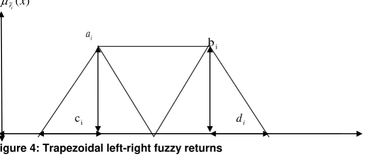
_i) by a (left-right) LR-fuzzy number of a trapezoidal form shown in Figure 4 below:

~(x)

i

r



a

i

i

[image:14.595.79.446.208.365.2]

c

d

i

Figure 4: Trapezoidal left-right fuzzy returns

Following Vercher (2007) we denote by

~

r

_i

(

a

_i

,

b

_i

,

c

_i

,

d

_i

)

_LRa LR-fuzzy return generated with strategy i;  a set of LR-fuzzy returns and





R

; where

a

_i

,

b

_i

,

c

_i

,

d

_iare real numbers on the trapeze representing the core spread [

a

_i



P40th ,

b

_i



P60th] and the extremes



i

c

P40th-P5th , and

d

_i



P95th-P60th where

Pk

th is the

k

th percentile of historical returns distribution. The following definitions apply.

Definition _{1: A fuzzy number}

i

r

~

_{is said to be a LR-fuzzy return i.e.}

LR i i i i

i

a

b

c

d

r

(

,

,

,

)

~

generated with strategyi, if and only if its membership function is defined by:

   

   

 

   

  

  

 

   

  

  

 

i i i

i i

i i

i i

i i

i

r~

d b x b if ; d

b x R

b x a if ; 1

a x c a if ; c

x a L

) x (

i ₍₂₄₎

where

a

_i



x



b

_iis the modal internal of real returns; L(.) and R(.) are reference linear functions strictly decreasing and upper semi-continuous defined from

[

,

0

[

]

1

,

0

[





to



respectively. These functions verify the condition of the trapezoidal symmetry such thatL(x)L(x); R(x) R(x)andL(0)R(0)1. According to Lodwich

i

14

and Bachman (2005) trapezoidal fuzzy numbers are a cut representation of any asymmetrical distribution of different shape forms

Definition 2_{: Let}

1

~

r

and

~

r

₂two fuzzy returns (generated with two different investment strategies 1 and 2); with membership functions ( )

1

~ x

r



and ( )

1

~ y

r



respectively, where

R y

x, ,



 . Following Vercher (2007) the possibility that the statement “return generated

with strategy 2 is higher than that generated with strategy 1,” is true is given by:



x y x y R x y



Sup

r r

Pos(~ ~) min( _r( ), _r ( ))/ ,  , 

2

1 ~

~ 2

1





(25)

In the same way the possibility that the statement “return generated with strategy 2 is the same as that generated with strategy 1,” is true is given by:



x y x y R



Sup

r r

Pos(~1 ~2) min(



r~₁( ),



r~₂( ))/ ,  . (26) The possibility that the statement “return generated with strategy 1 is less than the

manager’s targeted rate of returns



,” is true is given by:











  

 Sup x x R x

r

Pos(~1 ) min( r~₁( ))/ , . (27) The possibility that the manager has reached his/her targeted rates of return



with a given strategy is given by:

) ( ) ~ (





~



i r i r

Pos   . (28)

Definition 3_{: Let}

LR i i i i

i

a

b

c

d

r

(

,

,

,

)

~

1 1 1 1

1 and

r

i

(

a

i

,

b

i

,

c

i

,

d

i

)

LR

~

2 2 2 2

2 two fuzzy rates of return generated with two different investment strategies 1 and 2. The sum (subtraction and product) of two fuzzy rates of return is also a fuzzy number (Liu, 2004). In fact:

LR i i i i i i i i i

i

r

a

a

b

b

c

c

d

d

r

~

(

,

,

,

)

~

2 1 2 1 2 1 2 1 2

1













;

LR i i i i i i i i i

i

r

a

a

b

b

c

c

d

d

r

~

(

,

,

,

)

~

2 1 2 1 2 1 2 1 2

1













; (29)

       0 ) , , , 0 ) , , , ( ~























if c d a b if d c b a r LR i i i i LR i i i i

The alpha level set of a fuzzy return

~

r

_i

(

a

_i

,

b

_i

,

c

_i

,

d

_i

)

_LRgenerated with strategy i is a crisp subset of real numbers (R) denoted by:



x

x

x

R



r

i

r

i

]



/

(

)



,



~

15

second is the possibilitic expected mean of fuzzy numbers presented by Carlsson and Fuller (2001) which is consistent with the extension principle3 and is based on the set of alpha cuts. To obtain the fuzzy expected return for a given portfolio of hedge fund strategies we mimic Vercher (2006) by using membership function for each fuzzy return

~

r

_i

(

a

_i

,

b

_i

,

c

_i

,

d

_i

)

_LRfrom the power utility function (1 x) and evaluate all the shape parameters by means of ranking procedure (using percentile) of historical strategy returns.

If hedge fund strategy returns

r

~

_i(i1,2...n with n the number of investment strategies); are LR-fuzzy returns i.e.

~

r

_i

(

a

_i

,

b

_i

,

c

_i

,

d

_i

)

_LRwith different shape parameters; then the portfolio expected rate of return R~is given by:







n

i

w

i

r

i

R

~

₁

~

(31)



,

,

,





(

),

(

),

(

),

(

)



~

1

a

w

1

b

w

1

c

w

1

d

w

A

w

B

w

C

w

D

w

R





_in_{ i i}



n_{i i i}



_in_{ i i}



_in_{ i i}



(32) Equation (32) can be rewritten in matrix form as:



( ), ( ), ( ), ( )



~

w D w C w B w A

R  (33) where

w

represent a vector of investment capital allocated to investment strategyi. Following Dubois and Prade (1987), the interval-valued expected fuzzy mean return E(R~)is given by:



(~), (~)



) ~

(R E* R E* R

E  (34)

3

The Zadeh (1965) extension principle is a basic concept in the fuzzy set theory that extends crisp domains of mathematical

expressions to fuzzy domains. Suppose

f



.

is a function from X to Y and A is a fuzzy set on Xdefined as:

 

x

1

/

x

1

ma

 

x

2

/

x

2

...

ma

 

x

n

/

x

n

ma

A









where ma is the Membership Function of A. the



sign is a fuzzy OR (Max) and the

/

sign is a notation (indicated the variable

x

_i in discourse domain X - NOT DIVISION)

Then the Zadeh (1965) extension principle states that the image of fuzzy set A under the mapping

f



.

can be expressed as a fuzzy set B.

 

A

ma

 

x

1

/

y

1

ma

 

x

2

/

y

2

...

ma

 

x

n

/

y

n

f

B











16 whereE (R~) (Inf R~_)d



1

0

* 



; andE R Sup R)d



~ ( ) ~ ( 1 0 *



 ; are lower and upper bound of the interval respectively. Following Carlsson and Fuller (2001), the possibilitic expected fuzzy return R~is given by:



(~), (~)



) ~

(R M* R M* R

M  (35)

whereM (R~) 2



(Inf R~_)d



1

0

* 



; andM R



Sup R)d



~ ( 2 ) ~ ( 1 0 *



 ; are lower and upper bounds of the interval respectively. Bermudez et al. (2005) showed that the possibilistic expected mean is a subset of the interval-valued expected mean.

To model the risk associated with hedge fund investment we use a downside risk measure proposed by Leon et al. (2004) rather than the standard deviation. We believe that fund managers are more worried about the downside risk of their investment positions than the upper side. We view the downside risk as the failure of a manager to deliver on his/her promises. By definition the two downside risk measures corresponding respectively to interval-valued and possibilistic fuzzy returns are as follows:



0,E(R~) R~



] [max

E ) R~ (

V~1   (36)



0,M(R~) R~



] [max

E ) R~ (

V2   (37) Corresponding crisp functions of equations 34, 35, 36, and 37 can be obtained easily as in Vercher (2007) for an LR-fuzzy return

~

r

_i

(

a

_i

,

b

_i

,

c

_i

,

d

_i

)

_LR as follows:





        _{  }              _{  }  n

i i i i i

n

i ai bi di ci a b d c

R

E _{1 1} ( )

4 1 ) ( 2 1 ) ( 4 1 ) ( 2 1 , 0 max ) ~

( (38)





        _{  }              _{  }  n

i i i i i

n

i ai bi di ci a b d c

R

M _{1 1} ( )

6 1 ) ( 2 1 ) ( 6 1 ) ( 2 1 , 0 max ) ~

( (39)





_



_









_





































_

_

_



_ n

i i i i i

n

i

b

i

a

i

c

i

d

i

b

a

c

d

E

R

V

_{1 1 1}

(

)

2

1

)

(

2

1

)

(

,

0

max

)

~

(

(40)





_



_









_





































_

_

_



_ n

i i i i i

n

i

b

i

a

i

c

i

d

i

b

a

c

d

E

R

V

_{2 1 1}

(

)

3

1

)

(

3

1

)

(

,

0

max

)

~

(

(41)

17

) ~ (

) ~ (

1 R

V R E

PI  ; for an interval valued portfolio returns and; (42)

) ~ (

) ~ (

2 R

V R M

PP ; for a possibilistic portfolio returns. (43)

The portfolio with the highest PI (PP) measure will be the most preferred. Formulation of Investment Constraints under Fuzzy Set Theory

We present a bi-objective fuzzy set based investment allocation problem that minimises the downside risk while maximising the portfolio rate of return. The investment allocation problem is subjected to four different types of investment constraints, namely restriction on both short selling and leverage i.e.



n_i1

w

i



1

and

w

i



0

.

The second type of constraint restricts only short selling while giving the manager an unlimited leverage manoeuvre in order to achieve his/her targeted returns i.e.



_in_1

w

i



1

and

0



i

w

,or

w

i



0

.

The third type of constraint restricts only leverage while allowing the manager to use short selling i.e.



n_i1

w

i



1

, and

w

i



0

or

w

i



0

.

The fourth type of constraint gives the manager great margin of manoeuvre to use leverage and short selling in order to achieve his/her targeted rates of return i.e.



n_i1



1

or

w

i



0

or

0



i

w

.

The two crisp bi-objective strategies allocation problems that we want to optimize are:

 Problem 1: Interval-valued problem;

Maximize E R 



_in_1 a_i b_i  (d_i c_i)_w_i 4

1 ) (

2 1 )

~ (

Minimize V1 R 



_in_1 b_i a_i  (c_i d_i)_w_i 2

1 ) (

) ~ (

Subject to:

1.    

 







0 ,

0 1

1

i i

n i i

w w

18 2.      



 0 1 1 i n i i w w 3.



















0

w

,

0

w

1

w

i i n 1 i i 4.      



 0 1 1 i n i i w w

 Problem 2: Possibilistic problem:

Maximize M R 



_in_1 a_i b_i  (d_i c_i)_w_i 6 1 ) ( 2 1 ) ~ (

Minimize V R



n_i b_i a_i c_i d_i w_i

  

 _{  }

 ₁

2 ( )

3 1 ) ( ) ~ (

Subject to: 1.       



 0 , 0 1 1 i i n i i w w w 2.      



 0 1 1 i n i i w w 3.



















0

w

,

0

w

1

w

i i n 1 i i 4.      



 0 1 1 i n i i w w

where

w

i; represents the investment capital allocated to strategyi. We make use of the genetic algorithm to solve these bi-objective investment allocation problems.

Investment Allocation under Bayesian Settings

19

about the future expected returns distribution as new information comes into the markets. Furthermore, we extend the Bayesian portfolio selection model by presenting a counterpart model known as the Black-Litterman (1992) model.

We mimic Harvey, Liechty et al. (2004) who address both the estimation risk and the inclusion of higher moments in the portfolio selection. They suggest the use of skew normal distribution to capture the asymmetrical behaviour of returns. In this Bayesian framework, objective functions are optimized using predictive returns generated with the Monte Carlo Markov Chain (MCMC) simulations.

Suppose that a fund manager has a holding period of length



; the fund manager’s objective is to maximize his/her wealth at the end of the investment period

T





where Tis the sample period. Denote by



_Tthe unobserved next



periods’ expected returns; the predictive returns distribution can be written as (see Harvey, Liechty et al., 2004):











_



Y

p

Y

S

p

S

Y

d

d

dS

Y

p

(

T 

/

n

)

(

T 

/



,

,

)

(



,

,

/

n

)



(44)

where

Y

_nis a



T



N



matrix of historical returns of all investment strategies (

N

strategies) during the past T periods.

)

Y

/

S

,

,

(

p





_n is the joint posterior distribution of strategy returns assumed in this paper

to be a skewed student’s t-distribution with first, second and third moment given by

S and , ,



respectively. This distribution summarizes uncertainty about the future expected returns distribution.

)

,

,

/

(

Y

S

p

_T





is a multivariate skewed student’s t-distribution for the next



period future

expected returns. And : a proportionality sign.

We account for estimation risk by averaging in (44) over the posterior distribution of the parameters



,,andS. Therefore the distribution of

Y

T_will not depend on unknown parameters, but only on the past returns series

Y

_nassumed to be skewed student’s t -distribution.

The analytical solution of equation 44 is often difficult to obtain; often numerical methods such as the MCMC simulations (Metropolis-Hasting or the Gibbs sampler algorithm) are used to obtain the predictive distribution. In this paper the Gibbs sampler algorithm will be used for this purpose.

Substituting the predictive returns distribution into the fund manager’s objective functions,

20





























        

1

I

:

Subject to

)

/

(

)

~

'

(

max

)

/

(

)

~

'

(

min

)

/

(

~

'

max





















         T n T T W T n T T W T n T T W

dY

Y

Y

p

S

dY

Y

Y

p

dY

Y

Y

p

(45)

where



~

T_

,

~



_T

,

S

~

_T

,



,



,

and



is the predictive mean, predictive covariance matrix,

predictive coskewness matrix of future expected returns, aversion to change in risk, aversion to change in skewness, and the kronecker product.

To obtain the predictive moments of future expected returns, we use a skew t distribution derived from the skew elliptical class of distributions presented by Sahu et al. (2003). Its general form is shown to be:



















      X X g g X

f( / , , (P)) 1/2 (P) ' 1/2 ; X P (46)

with ; where;a 0; ( , ) 0

) , ( ) , ( ) 2 / ( ) ( 0 1 2 0 1 2 2 / ) (    





 _

 _ r g r p dr

dr p r g r p u g p u g P P p P



Sahu et al. (2003) show that when

(

,

)

1

2

;

(with

0

)

) (













 



 





 P

u

p

u

g

equation (46)

becomes a multivariate student’s t-distribution under the condition that the vector of random variables X is transformed as follows:





 

 DZ

X (47) where Zis a vector of unobservable random variables whose distribution is elliptical with mean zero and identity covariance matrix I_p ;







Pvector of mean; D, is a ppmatrix of skewness and co skewness:































pp p p p p

D



















....

:

....

:

:

....

....

2 1 2 22 21 1 12 11 ;

with



_ij : representing the coskewness of random variable

x

_iand x_jfor all

i



j

; and skewness for

i



j

; and



a vector of error terms defined as



st(0,,



)(i.e. skewed t-student random variable). Consequently Sahu et al. (2003) show that the conditional distribution of random variable Y (X /Z 0)given



,,D,and



has the following

21 ) , / ( , 2 ) , , , /

(Y D t Y D2

p







  _





 (48) where

V

follows student’s t-distribution,

t

_

,







.

It is now possible to implement a Bayesian portfolio selection under the assumption that

hedge fund returns have a skewed student’s t-distribution. This implementation is done using

the MCMC simulations with a Gibbs sampler that requires us to first specify the likelihood function, the priors and posteriors distribution before computing the predictive moments of future expected returns.

Following German and German (1984) the likelihood of the data can be specified as

        _    w Dz w D z

y_i/ _i,



, , , _i N_p



_i, (49)

where 

        2 , 2 w and ; ) , 0 ( i





P p

i N I

z

For the informative priors scenario we consider the conjugate priors distribution for the unknown parameter



given ,



,andD; and the unknown parameter  which has a multivariate inverted Wishart distribution as in Harvey et al. (2004):

) , ( ) , ( ) , ( ) , (   









              d N D C W Inv m N p p p (50)

Notice that



is a parameter that adjusts the degree of our beliefs about the skewness in the distribution of the data, a prior value of this parameter must be specified in the informative prior settings; it goes the same with the mean vector

d

which reflects our prior information. Following Polson and Tew (2000), and Harvey et al. (2004), we then obtain the predictive moments of future expected distribution as

) / ) ~ ( ) ~ ( ~ ) / ( 3 ) / ( 3 ~ ) / var( ~ ~ Y m m E Y V E Y m V E S S Y m T T T T T T      











                    (51)

where



~

T_

,



~

_T

,

~

S

_Tare the predictive (central) moments, and



,,S are the posterior