http://www.scirp.org/journal/ajcm ISSN Online: 2161-1211
ISSN Print: 2161-1203
Computational Modeling and Dynamics of the
Oil and Water Flow Using the Galerkin
Approximation
Ferdusee Akter1, Ujjwal Kumar Deb2*
1Department of Physical and Mathematical Sciences, Chittagong Veterinary and Animal Sciences University, Chittagong, Bangladesh
2Department of Mathematics, Chittagong University of Engineering & Technology, Chittagong, Bangladesh
Abstract
A Computational Fluid Dynamic (CFD) model is presented to analyze the flow dynamics of a two phase incompressible flow in the application sectors of different industries. The Finite Element method (FEM) which is based on the Galerkin approximation, has been implemented for this two phase flow mod-el. Generally, two-phase flows can occur in different forms like gas-liquid, liq-uid-liquid and solid-liquid forms. The Oil and Water two-phase flow is an important phenomenon in petroleum industry for crude oil production and transportation. In our study, a laminar flow of liquid-liquid phase is consi-dered to simulate the flow dynamics where the liquid phases are water and oil. The COMSOL Multiphysics software is used to perform the simulation in-cluding velocity profile, volume fraction, shear rate, pressure distributions and interfacial thicknesses at different times. A typical circular tube domain with radius 0.05 m and length 8 m is assumed for our simulation.
Keywords
Two-phase Flow, CFD, Galerkin Method, FEM, Simulation
1. Introduction
The two-phase flows are found widely in the nature and in a whole range of in-dustrial applications. The two-phase material is often called the mixture [1]. In a single phase flow, the design parameter can be modeled easily but the presence of a secondary phase increases the complexity of the fluid flow. The two phase flow phenomena is still difficult to understand because of their complex behavior [2]. With the progress of science and technology, the study of mathematical models
How to cite this paper: Akter, F. and Deb, U.K. (2017) Computational Modeling and Dynamics of the Oil and Water Flow Using the Galerkin Approximation. American Journal of Computational Mathematics, 7, 58-69.
https://doi.org/10.4236/ajcm.2017.71005
Received: January 18, 2017 Accepted: March 28, 2017 Published: March 31, 2017
Copyright © 2017 by authors and Scientific Research Publishing Inc. This work is licensed under the Creative Commons Attribution International License (CC BY 4.0).
which may describe the two-phase flow phenomena has taken an increasing atten-tion and becomes a challenge to the researcher [3] [4] [5].
A variety of two-phase flows can occur depending on the combination of two-phases such as gas-liquid, liquid-solid, liquid-liquid and gas-solid. Generally, we see these two phase flows in transport of oil-gas mixtures in the pipeline sys-tem, air conditioning and refrigeration syssys-tem, crystallization syssys-tem, clay extrac-tion, oil water mixture flow in pipelines and fuel combustion etc.
There are various studies which have been done on two phase flow. Aparallel streamline Upwind Petrov-Galerkin model using the Finite Element method for two-phase flow in a T-junction showed that the primary phase accumulates at the middle of the pipe and top of the wall while the secondary phase accumulates near the wall after the junction [6]. In an air-oil flow, it was found that oil was concen-trating at the lower portion of pipe’s cross section due to gravity. A wave of oil and air mixture was present at the middle that covers the whole pipe cross section area and a new wave of the mixture was just entering the pipe segment [7]. A mathe-matical model of gas liquid incompressible fluid flow was introduced to explore the feature of fluid under certain centrifugal force in vertical centrifugal casting using the projection level set method and showed that the free surface near the wall was higher compared to other parts of the domain. The distribution of liquid phase calculated by the projection level set method coincided with the physical truth and the pressure distribution was found a parabola [8]. So many types of flow patterns were predicted at different phase velocities of the flow of two im-miscible liquids through the horizontal pipelines using volume of fluid method. The slug flow appeared at low velocities while in annular flow, the total pressure of the mixture decreases with the increases of the oil velocity. It is found that the vo-lume fraction of oil is maximum at the centre in a core annular flow and at the upper side of the pipe in case of stratified flow [2]. In a stratified oil-water two-phase flow the pressure gradient increases as the velocity increases [9]. The water phase accumulates at the bottom of the pipe for low velocities in a horizontal pipe [10]. Solid phase velocity profile is asymmetrical about the central axis and maximum velocity position moves toward the top of the pipe in a solid-liquid slurry flow [11]. The high velocity region is observed at the outer side of the pipe in a CFD simulation of two-phase flow in helical pipe using population balanced model [12]. The radial velocity of a dispersed phase is larger than that of a gaseous phase. Also lighter and smaller ash particles move faster than corundum particles of same mass [13]. For different inlet velocities, pressure loss was different in two-phase flow of vertical pipe and increasing gas velocity reduced the total pres-sure loss in the pipe [14].
be applied using irregular grid of various shapes. It also provides a set of functions which give the variation of differential equations between the grid points [15].
The oil-water flow is very common in the petroleum industries. Generally the oil phase is transported in a multiphase flow condition as water and oil are nor-mally produced together. The presence of water has a significant effect during the transportation of oil. The complex interfacial structure of oil water flow makes it difficult to predict the hydrodynamics of the fluid flow [10] [16]. A comparison was done for the different shape of photo bioreactor for Microalgae culture and we considered the tubular one is better [17].
In literature, we found different models for two-phase flows including the Pe-trov-Galerkin method, the projection level set method, the volume of fluid me-thod, and the population balanced model.
In our study, we considered a FEM model for two-phase flow using the Galerkin method and an oil-water mixture flow is taken to simulate according to our model. To investigate the velocity profile, the volume fraction and the pressure distribu-tion of the oil-water two-phase flow through a circular tube we applied boundary and initial condition in the inlet, outlet and wall of a typical computational do-main.
2. Mathematical Model Formulation
In this section, a mathematical model will be developed to discuss the two-phase flow. A computational domain will also be constructed to simulate the fluid flow. A suitable mesh design is considered as the computational domain. The in-itial and boundary conditions are for the oil-water two-phase flow in a phase field platform.
2.1. Governing Equations
In this study, we consider a two-phase incompressible Newtonian flow in which the phases are liquid and the flow mixture is laminar. Therefore, the governing equation of the problem becomes as follows along with Boundary Conditions (BC) and Initial conditions (IC) in the computational domain Ω,
0
∇ ⋅ =u (1)
(
)
(
T)
, st p
t
ρ∂ + ⋅∇ = −∇ + ∇ ⋅ µ ∇ + ∇ +ρ + ∂
u
u u u u g F (2)
where u denotes the velocity of the mixture, ρ and µ are its density and viscosity respectively, g is the gravity and Fst is the surface tension force. The phase field variable [18] ϕ is governed by the following partial differential
equation (PDE)
G t
ϕ ϕ γ
∂ + ⋅∇ =∇ ⋅ ∇
∂ u , (3)
where G is the chemical potential.
2
t
ϕ ϕ γλ ψ
ε ∂
+ ⋅∇ = ∇ ⋅ ∇
∂ u , (4)
(
)
22 2
1 ε f
ψ ε ϕ ϕ ϕ
λ ϕ
∂
= −∇ ⋅ ∇ + − +
∂
, (5)
where ϕ is the dimensionless phase field variable, γ is the mobility, ε is a
controlling interface parameter, λ is the mixing energy density, the term f
ϕ
∂ ∂
denotes the ϕ derivative of external free energy and χ is the mobility tuning
parameter. The density and viscosity of the mixture are the function of volume fraction of water Vw. The volume fraction of water and oil are
1 2 w
V = +ϕ and 1
2 o
V = −ϕ respectively. The density and dynamic viscosity of the two-phase model are calculated over the interface according to
(
)
o w o Vw
ρ ρ= + ρ −ρ (6)
(
)
o w o Vw
µ µ= + µ −µ , (7) where the subscript w and o are used for water and oil respectively. The surface tension force for the method is applied as a body force
st = ∇G ϕ
F . (8) The chemical potential G is given by the following equation related to the phase field variable and the interface controlling parameter.
(
2)
2
2
1 G λ ϕ ϕ ϕ
ε
−
= −∇ +
. (9)
2.2. Initial and Boundary Conditions for the Simulation
As the mixture of oil and water is incompressible, the flow is assumed to be la-minar two-phase flow where the volume fraction of water and oil are considered 0.91 and 0.09 respectively [20]. The phase field method gives better interface than other methods. In phase field method, the interfacial layer is governed by a phase field variable which is obtained from the Cahn-Hilliard equation. The COMSOL Multiphysics software is used for the CFD simulation. At the inlet we considered velocity u =u0, a no slip boundary condition on the wall and the
traction boundary condition were imposed at the outlet which are given by 0
=
u (10)
= ⋅ =
T σ n T, where σ= − +pI µ
(
∇ + ∇u uT)
(11)2.3. Computational Domain and Mesh Design
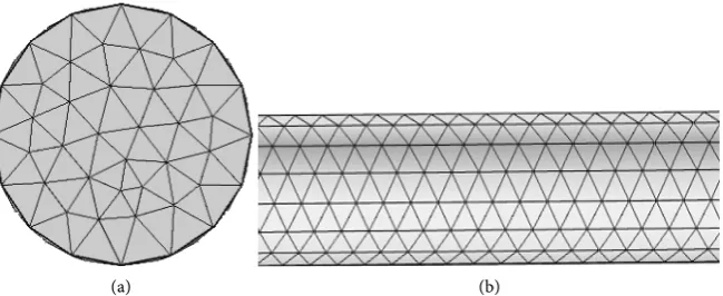
Atypical circular tube domain as in Figure 1 is considered in our study with 8 m length and 0.05 m radius while the working volume and surface area are 0.0618 m3 and 2.518 m2 respectively. As the mesh design plays a significant role in
with 81,143 elements and 619,748 degrees of freedom according to Figure 2.
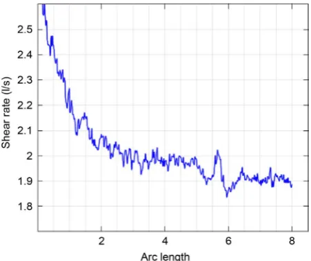
3. Finite Element Approximation
The variational statement of a boundary value problem is the integral represen-tation of the problem. We can obtain the variational statement by setting the to-tal weighted residual error to zero. When the local residual error is multiplied by a weighting function and then integrating over the domain, the weighted resi-dual error is obtained [15]. The aim is to find an approximate solution such that the total weighted residual error vanishes. If the weighting functions are same as the basis functions, the method is known as Galerkin method. The finite element method is used to calculate the basis functions for the Galerkin approximation of the boundary value problem.
3.1. Variational Statement
( )
(
(
T)
)
, st
x t p
t
ρ∂ µ ρ
= + ⋅∇ + ∇ − ∇ ⋅ ∇ + ∇ − −
∂
u
r u u u u g F (12)
[image:5.595.211.541.366.551.2] [image:5.595.213.538.581.714.2]According to weighted residual method [15] there is
(
u,p)
∈ ×V Q such that for every t∈IFigure 1. The geometry of the computational flow domain.
(a) (b)
( )
r v, =0 ∀ ∈v V and v=0 on Γu (13)(
∇ ⋅u,q)
= ∀ ∈0, q Q (14)( )
, 0 = 0u x u in
Ω
(15) in u= Γ
u u (16) where V and Q are velocity and pressure spaces and the inner product is defined by
( )
, dΩ
=
∫
⋅ Ωa b a b (17) The integral representation of (13) is presented as follows
(
)
(
T)
d d d st d d
D
p s
Dt
ρ µ ρ
Ω Ω Ω Ω ∂Ω
⋅ Ω + − ∇ ⋅ + ∇ + ∇ ∇ Ω − ⋅ Ω − ⋅ Ω = ⋅
∫
u v∫
v u u v∫
g v∫
F v∫
T v (18)Since ∂Ω = Γ ∪ Γu t and u is specified on Γu and v is chosen to be zero on Γu.
The variational statement of the problem is,
(
)
(
)
(
(
)
)
(
) (
)
( )
(
)
( )
( )
{
}
{
}
( )
{
}
T 0 0 2 1 0 1Find , such that for every
, , , , , ,
, 0, , 0 in
on
, and 0 on
st
u
u
p Q t I
D
p b
Dt
q q Q
H V
Q H
ρ µ ρ
β β ∈ × ∈ − ∇⋅ + ∇ +∇ ∇ − − = ∀ ∈
∇ ⋅ = ∀ ∈ = Ω
= Γ
= ∈ Ω = ∈ = Γ
= ∈ Ω
u V
u
v v u u v g v F v T v v V
u u x u
u u
V v v v v V v
(19)
This variational statement is also known as the weak formulation of a two-phase Newtonian incompressible flow in a computational domain
Ω
. 3.2. The Galerkin Finite Element ApproximationTo find the Finite Element approximation, let Vh ⊂V be a N-Dimensional subspace of V with basis functions
{
φ φ1, 2,,φN}
. Approximating v and q in (19) by1
N h k k
k v φ =
=
∑
v and
1
M p p p q θ q
= =
∑
(
)
(
(
T)
)
(
) (
)
(
)
1
, , , , , ,
0
N
k k k k st k k k
k
D
p b v
Dt
ρ φ φ µ φ ρ φ φ φ
= − ∇⋅ + ∇ +∇ ∇ − − − =
∑
uu u g F T
(20)
(
)
1 , 0 M p p p q θ = ∇ ⋅ =∑
u (21)which can be written as
(
) (
)
(
(
)
)
(
) (
)
(
)
T
, , , ,
, , ,
k k k k
k st k k
p t
b
ρ φ ρ φ φ µ φ
ρ φ ϕ φ
∂ + ⋅∇ − ∇ ⋅ + ∇ + ∇ ∇ ∂ = − − u
u u u u
g F T
(
∇ ⋅u,θp)
=0 (23) Now approximating u and p respectively by1
N h l l
l u φ = =
∑
u and
1
M
h p p
p
p ω p
= =
∑
Therefore, we get from (22) and (23) that
(
)
(
)
(
)
(
)
{
}
(
)
(
) (
)
(
)
T T 1 1 , , , , , , , , Nl k l l l k l l k l l k l
l M
p k p k st k k
p
u u u u
p b
ρφ φ ρ φ φ φ µ φ φ µ φ φ
ω φ ρ φ φ φ
=
=
+ ⋅∇ + ∇ ∇ + ∇ ∇
− ∇ ⋅ = + +
∑
∑
g F T (24)
(
)
1 , 0 Nk p k k
u φ ω =
∇ ⋅ =
∑
(25)which can be represented by
T T T
1 1 2 2 3 3 0
M A CP
C U C U C U
+ − =
− − − =
U U F
using M =
( )
mkl with mkl =(
ρφ φk, l)
( )
klD= D with Dkl =
(
ρφl⋅∇φ φl, k)
(
,)
ij ijkl k l
K =K = µ φ∇ ∇φ
ij A=K +D
ikp
C=C with Cikp =
(
ωp,∇ ⋅φk)
ik
=
F F with Fik =
(
ρ φg, k) (
+ Fst,φk)
+b(
T,φk)
(
)
, 1, 2, ,
k l= N and i j, =1, 2, 3
4. Numerical Results and Discussion
[image:7.595.202.541.69.490.2]In our study, COMSOL Multiphysics version 4.2 has been used to simulate the oil-water two-phase flows. Properties of the fluid phases and parameters values are given in Table 1 [9] and Table 2 [18] respectively. The zero normal stress is considered at the outlet in our simulation. We have analyzed the velocity mag-nitude, the volume fractions of fluids, the pressure and the shear rate distribu-tions for this two-phase flow mixture. It is also notable that as we simulated a two-phase flow, the interface thickness is an important criterion to understand the general state of the mixture. In this part we discuss about the oil-water inter-faces for different times.
Table 1. Physical properties of fluid phases.
Property Symbol Water phase Oil phase
Density ρ 998.2 kg/m3 780 kg/m3
Dynamic viscosity µ 0.001003 Pa∙s 0.00157 Pa∙s
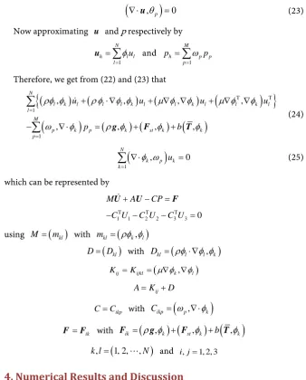
The Figure 3(a) shows the slices of the velocity magnitude while the Figure 3(b) represents their corresponding line graph at three different cross sections of the horizontal pipe at x=1 m, x=4 m and x=7 m respectively. It is found that velocity magnitude is generally higher at the middle part of the tube and the lowest at the boundary of the tube. The velocity profiles form a parabolic shape showing the maximum velocity at the center.
Table 2. Parameters value used for simulation.
Symbol Quantity Values
0
u Inlet initial velocity 0.024 m/s
f ϕ ∂
∂ Phi-derivative of external free energy 0.01 J/m
ε Parameter controlling interface thickness 0.01 m
χ Mobility tuning parameter 1 m∙s/kg
g Gravity 9.8 m/s2
i) Velocity magnitude at x = 1 m ii) Velocity magnitude at x = 4 m iii) Velocity magnitude at x = 7 m (a)
(b)
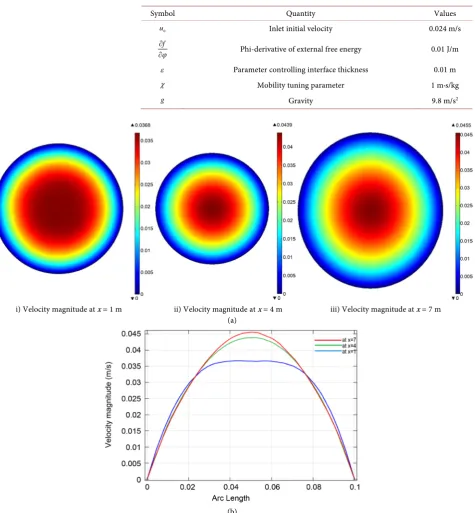
In case of fluid flow inside a tube domain the shear stress can be found on the wall of the domain. We investigated the shear rate distribution for the entire domain which is shown in Figure 4. It shows the shear rate decreases gradually with small fluctuations along the domain.
One of the important parameters used to characterize the two-phase flow is the volume fraction of different phases. Figure 5(a) and Figure 5(b) shows the volume fraction of the oil and the water phase respectively along the horizontal pipe. We see that in the mixture the volume of the oil phase sharply increased while the water phase decreased at the same ratio.
Figure 6 represents the pressure drop along the pipe. A linear pressure drop is observed from the inlet to the outlet though there is a sudden drop near the in-let. This indicates the velocity of the mixture is increased initially and it keeps remain until the end of the tube.
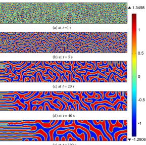
[image:9.595.261.487.305.494.2]The Figure 7 represents the oil-water interfaces at different times of our si-mulation. At the beginning of the mixture, the two-phases are mixed completely
Figure 4. The shear rate distribution along the domain.
[image:9.595.89.540.524.711.2](a) The Volume Fraction of Oil (b) The Volume fraction of Water
Figure 6. The pressure distribution along the domain.
Figure 7. The oil-water interfaces at different times of the mixture.
except for a small change around zero of the value of the phase field variable. The phases have started to separate (Figure 7(b)) at t = 1 s. After that the oil and water phases have started to form different phases (Figure 7(c) and Figure 7(d)) according to the phase field variable and we observed the two-phases exist sepa-rately. Gradually, the phases formed large phase domains by creating an inter-face to separate the phases. This shows that the two fluids tend to separate into distinct phases.
5. Conclusion
[image:10.595.229.519.246.533.2]the variational statement of the fluid flow problem by setting the total weighted residual error to zero. A computational domain with 8 m length and 0.05 m ra-dius respectively is constructed to simulate an oil-water two-phase flow. The ve-locity magnitude has been observed higher at the middle of the tube and the lowest at the boundary of the tube. The shear rate decreased with small fluctua-tion along the domain. The Oil phase volume fracfluctua-tion increased consequently the water phase decreased at the same ratio. From the inlet to the outlet, a linear pressure drop is observed. It is also notable that the fluids tend to separate into two distinct phases.
Acknowledgements
The authors gratefully acknowledge for the technical support to The Centre of excellence in Mathematics, Department of Mathematics, Mahidol University, Bangkok, Thailand.
References
[1] Drew, D.A. (1983) Mathematical Modeling of Two-Phase Flow. Annual Reviews on
Fluid Mechanics, 15, 261-291. https://doi.org/10.1146/annurev.fl.15.010183.001401
[2] Desamala, A.B., Dasamahapatra, A.K. and Mandal, T.K. (2014) Oil-Water Two-phase Flow Characteristics in Horizontal Pipeline A Comprehensive CFD Study. International journal of Chemical, Molecular, Nuclear, Materials and
Metal-lurgical Engineering, World Academy of Science, Engineering and Technology, 8,
360-364.
[3] Liao, Q., Liu, D., Ye, D., Zhu, X. and Lee, D. (2011) Mathematical Modelling of Two-phase Flow and Transport in an Immobilized-Cell Photo Bioreactor.
Interna-tional Journal of Hydrogen Energy, 36, 13939-13948.
[4] Morin, A. (2012) Mathematical Modelling and Numerical Simulation of Two-phase Multi-component Flows of CO2 Mixtures in Pipes. PhD Thesis, Norwegian Univer-sity of Science and Technology, Norway.
[5] Hudson, J. and Harris, D. (2006) Numerical Modeling of Eulerian Two-Phase Gas-Solid Flow. Manchester Institute of Mathematical Sciences, Manchester, 1-41. [6] Giordano, M., Bonfiglioli, A. and Magi, V. (2006) A Parallel Finite Element Method
for Two-phase Flows. European Conference on Computational Fluid Dynamics, Glasgow, 1-20.
[7] Kanarachos, S. and Flouros, M. (2014) Simulation of Air-Oil Mixture Flow in the Scanvenge Pipe of an Aero Engine Using Generalized Interface Momentum Ex-change Model. WSEAS transaction on Fluid mechanics, 9, 144-153.
[8] Zhou, J.X., Shen, X., Yin, Y.J., Gou, Z. and Wang, H. (2015) Gas Liquid Two-phase Flow Modelling of Incompressible Fluid and Experimental Validation Studies in Vertical Centrifugal Casting. IOP Conference Series: Material science and
Engi-neering, 84, 1-9. http://dx.doi.org/10.1088/1757-899X/84/1/012042
[9] Alias, A.Z.M., Koto, J. and Ahmed, Y.M. (2015) CFD Simulation for Stratified Oil-Water Two-Phase Flow in a Horizontal Pipe. International Society of Ocean,
Mechanical and Aerospace Scientists and Engineers, 2, 1-6.
[10] Hu, H. and Cheng, Y.F. (2016) Modelling by Computational Fluid Dynamics Simu-lation of Pipeline Corrosion in CO2-Containing Oil-Water Two-phase Flow. Journal
[11] Nabil, T., EL-Sawaf, I. and EL-Nahhas, K. (2013) Computational Fluid Dynamics Simulation of the Solid-Liquid Slurry Flow in a Pipeline. Seventh International
Wa-ter Technology Conference, 5-7 November 2013, Istanbul, Turkey.
[12] Rathod, R and Hebbal, O. (2013) CFD Simulation of Two-phase Flow and Heat Transfer in Helical Pipe. International Journal of Engineering Research and
Tech-nology, 2, 2150-2157.
[13] Kartushinsky, A., Siirde, A., Rudi, U. and Shablinsky, A. (2011) Mathematical Mod-el of Two-phase Flows Loaded with Light and Heavy Particles to Analyze CFB Processes. Oil Shale, 28, 169-180. http://dx.doi.org/10.3176/oil.2011.1S.09
[14] Sanati, A. (2015) Numerical Simulation of Air-Water Two-phase Flow in Vertical Pipe Using k-ε Model. International Journal of Engineering and Technology, 4, 61-70. https://doi.org/10.14419/ijet.v4i1.3965
[15] Yu, W.H. and Wiwatanapattaphee, B. (2006) Finite Element Method and Applica-tion. Mistercopy Publishing Company, Bangkok.
[16] Abed, E.M. and Auda, Z.A. (2014) Simulation and Experiment of Oil-Water Flow with Effect of Heat Transfer in Horizontal Pipe. International Journal of Mechanical
Engineering and Applications, 2, 117-127.
http://dx.doi.org/10.11648/j.ijmea.20140206.16
[17] Shahriar, M., Monir, M.I. and Deb, U.K. (2016) Comparative Analysis of Hydrody-namics Behavior of Microalgae Suspensio Flow in Circular, Square and Hexagonal-Shape Photo Bio-Reactors. America Journal of Computational Mathematics, 6, 320 -335. http://dx.doi.org/10.4236/ajcm.2016.64033
[18] Deb, U.K., Chayantrakom, K., Lenbury, Y. and Wiwatanapataphee, B. (2012) Nu-merical Simulation of Two-Phase Laminar Flow for CO2 and Microalgae Suspen-sion in the HLTP. Latest Advances in System Science and Computational
Intelli-gence,WSEAS Press, Haifa, 53-58.
[19] Cahn, J.W. and Hilliard, J.E. (1958) Free Energy of a Non-Uniform System in In-terfacial Energy. Journal of Chemical Physics, 28, 258-267.
https://doi.org/10.1063/1.1744102
[20] Xu, X. (2007) Study on Oil-Water Two-Phase Flow in Horizontal Pipelines. Journal
of Petrolium Science and Engineering, 59, 43-58.
Submit or recommend next manuscript to SCIRP and we will provide best service for you:
Accepting pre-submission inquiries through Email, Facebook, LinkedIn, Twitter, etc. A wide selection of journals (inclusive of 9 subjects, more than 200 journals)
Providing 24-hour high-quality service User-friendly online submission system Fair and swift peer-review system
Efficient typesetting and proofreading procedure
Display of the result of downloads and visits, as well as the number of cited articles Maximum dissemination of your research work
Submit your manuscript at: http://papersubmission.scirp.org/