Spatial panel data models with common shocks

Munich Personal RePEc Archive

Spatial panel data models with common

shocks

Bai, Jushan and Li, Kunpeng

December 2013

Online at

https://mpra.ub.uni-muenchen.de/52786/

Spatial panel data models with common shocks

Jushan Bai∗ and Kunpeng Li†

March 9, 2014

Abstract

Spatial effects and common-shocks effects are of increasing empirical importance. Each type of effect has been analyzed separately in a growing literature. This pa-per considers a joint modeling of both types. Joint modeling allows one to determine whether one or both of these effects are present. A large number of incidental param-eters exist under the joint modeling. The quasi maximum likelihood method (MLE) is proposed to estimate the model. Heteroskedasticity is explicitly estimated. This paper demonstrates that the quasi-MLE is effective in dealing with the incidental parameters problem. An inferential theory including consistency, rate of convergence and limiting distributions is developed. The quasi-MLE can be easily implemented via the EM al-gorithm, as confirmed by the Monte Carlo simulations. The simulations further reveal the excellent finite sample properties of the quasi-MLE. Some extensions are discussed.

Key Words: Panel data models, spatial interactions, common shocks, cross-sectional dependence, incidental parameters, maximum likelihood estimation

∗_{Department of Economics, Columbia University, New York, NY, 10027. Email: [email protected]} †_{School of International Economics and Management, Capital University of Economics and Business,}

Beijing, China. email: [email protected].

An earlier version of this paper is available at SSRN with link:

1

Introduction

There is a large and yet still rapidly growing literature on spatial interactions and common shocks, both of which lead to cross-sectional dependence. In spatial models, the cross sec-tional dependence is captured by spatial weights matrices based either on physical distance, and relative position in a social network or on other types of economic distance. The cross-sectional dependence in a common-shocks model arises from the response of individuals to the shocks. The common shocks model is characterized by a common factor structure. All these models are motivated by empirical considerations.1 The existing literature largely analyzes the two types of models separately. This paper integrates spatial interactions and common shocks. We show that the maximum likelihood method is an effective way of estimating the resulting model.

Early development of spatial models has been summarized by a number of books, including Cliff and Ord (1973), Anselin (1988), and Cressie (1993). GMM estimation of spatial models are studied by Kelijian and Prucha (1998, 1999, 2010), and Kapoor et al. (2007), among others. The maximum likelihood method is considered by Ord (1975), Anselin (1988), Lee (2004a), Yu et al. (2008) and Lee and Yu (2010), and so on. For panel data models with multiple common shocks, Ahn et al. (2013) consider the fixed-T GMM estimation. Pesaran (2006) proposes the correlated random effects method by including additional regressors, which are the cross-sectional averages of dependent and the explanatory variables. The principal components method is studied by Bai (2009) and Moon and Weidner (2009). Bai and Li (2014) consider the maximum likelihood method.

The joint presence of spatial interactions and common shocks calls for a different esti-mation procedure, as the existing method is not directly applicable. Under joint modeling, there exist a large number of incidental parameters. This paper also allows cross sec-tional heteroskedasticity, giving rise to further incidental parameters. We show that the maximum likelihood method can effectively deal with the incidental parameters.

This paper considers the following spatial panel data model with common shocks, in which both the dependent variablesyit and the explanatory variablesxit are impacted by

the common shocksft:

yit=αi+ρ N

X

j=1

wij,Nyjt+ k

X

p=1

xitpβp+λ′ift+eit,

xitp=νip+γip′ ft+vitp, p= 1,2, . . . , k;

(1.1)

whereyit is the dependent variable; xit= (xit1, xit2, . . . , xitk)′ is ak-dimensional vector of

explanatory variables;ft is anr-dimensional vector of unobservable common shocks;λi is

the corresponding heterogenous response to the common shocks; WN = (wij,N)N×N is a

specified spatial weights matrix whose diagonal elementswii,N are 0; andeitandvitare the

1_{For spatial interaction and economic distance, see, e.g., Case (1991), Case et al. (1993), Conley (1999),}

idiosyncratic errors. In model (1.1), the termλ′

iftcaptures the common shock effects, and

ρPN

j=1wij,Nyjt captures the spatial effects. The joint modeling allows one to test which

type of effects is responsible for the cross sectional dependence. We may testρ= 0 while allowing common shocks. Similarly, we may determine if the number of factors is zero in a model with spatial effects. It may be possible that both effects are present.

An additional feature of the model is the allowance of cross sectional heteroskedasticity. The importance of permitting heteroskedasticity is noted by Kelejian and Prucha (2010) and Lin and Lee (2010). The heteroskedastic variances can be empirically important, e.g., Glaeser et al. (1996) and Anselin (1988). In addition, if heteroskedasticity exists but homoskedasticity is imposed, then MLE can be inconsistent. Under large N, the consistency analysis for MLE under heteroskedasticity is challenging even for spatial panel models without common shocks, owing to the simultaneous estimation of a large number of variance parameters along with (ρ, β). The existing quasi maximum likelihood studies, such as Yu et al. (2008) and Lee and Yu (2010), typically assume homoskedasticity. These authors show that the limiting variance of MLE has a sandwich formula unless normality is assumed. Interestingly, we show that the limiting variance of the MLE is not of a sandwich form if heteroskedasticity is allowed.

Spatial correlation and common shocks are also considered by Pesaran and Tosetti (2011), who specify the spatial autocorrelation on the unobservable errors eit while we

specify the spatial autocorrelation on the observable dependent variableyit. Both

specifi-cations are of practical relevance. Spatial specification on observable data makes explicit the empirical implication of the coefficient ρ. From a theoretical perspective, the spatial interaction on the dependent variable gives rise to the endogeneity problem, while the spa-tial interaction on the errors, in general, does not. As a result, under the Pesaran and Tosetti setup, existing estimation methods on the common shocks models such as Pesaran (2006) and Bai (2009) can be applied to estimate the model. As a comparison, these methods cannot be directly applied to model (1.1) due to the endogeneity from the spatial interactions.

In this study, we consider the pseudo-Gaussian maximum likelihood method (MLE), which simultaneously estimates all parameters of the model, including heteroskedasticity. We give a rigorous analysis of the MLE including the consistency, the rate of convergence and limiting distributions. The asymptotic theory does not rely on normality.

In subsequent exposition, the matrix norms are defined in the following way. For any m_×nmatrixA,_kA_kdenotes the Frobenius norm of A, i.e., _kA_k= [tr(A′_A)]1/2_,kAk

2 the

spectral norm, i.e., _kA_k2 = [λmax(A′A)]1/2, where λmax(·) denotes the largest eigenvalue.

In addition, _kA_k∞ is defined as kAk∞ = max1≤i≤mPnj=1|aij| and kAk1 is defined as

kA_k1 = max1≤j≤nPmi=1|aij|, where aij is the (i, j)th element of A. We use ˙at to denote

˙

at=at−_T1 PTt=1atfor any column vectoratandMab to denote _T1 PTt=1a˙tb˙′tfor any vectors

at and bt.

(1.1) and the assumptions needed for the subsequent analysis. Section 3 presents the objective function and the associated first order conditions. The asymptotic properties including the consistency, the convergence rates and the limiting distributions are derived in Section 4. Computing algorithm is discussed in Section 5. Section 6 reports simulation results. Section 7 discusses extensions of the model. The last section concludes. Technical proofs are given in a supplementary document.

2

Model description and assumptions

Let vit = (vit1, vit2, . . . , vitk)′ and νi = (νi1, νi2, . . . , νik)′, and let γi = (γi1, γi2, . . . , γik).

Thex equation in model (1.1) is equivalent to

xit=νi+γi′ft+vit.

Now model (1.1) can be rewritten as

"

yit−ρPNj=1wij,Nyjt−x′itβ

xit

#

=µi+ Φ′ift+ǫit

with Φi = [λi, γi],µi = [αi, νi′]′ and ǫit= [eit, v′it]′. LetD(ρ, β) be an N(k+ 1)×N(k+ 1)

matrix, whose (i, j) subblock, denoted byDij(ρ, β), is equal to

Dij(ρ, β) =

            

"

1 ₋β′

0 Ik

#

if i=j

"

−ρwij,N 0

0 0

#

if i₆=j

(2.1)

Now model (1.1) can be further written as

D(ρ, β)zt=µ+ Φft+ǫt (2.2)

where zt = (z1t, z2t, . . . , zN t)′ with zit = (yit, xit′ )′, Φ = (Φ1,Φ2, . . . ,ΦN)′, µ = (µ′1, µ′2,

. . . , µ′

N)′andǫt= (ǫ′1t, ǫ2′t, . . . , ǫ′N t)′. Hereafter, we suppressρ, βfromD(ρ, β) for notational

simplicity. Throughout the paper, we assume that the number of factors r is fixed and known. Determining the number of factors is discussed in Section 6, where a modified information criterion of Bai and Li (2014) is proposed. Our simulation results are based on the estimated number of factors.

To analyze model (1.1), we make the following assumptions. Comments on these as-sumptions are given in a number of remarks below.

Assumption A: The ft is a sequence of constants. Let Mff =T−1PTt=1f˙tf˙t′, where

˙

ft = ft− _T1 PTt=1ft. We assume that Mff = limT→∞Mff is a strictly positive definite

matrix.

B.1 Theeit is independent and identically distributed overtand uncorrelated overiwith

E(eit) = 0 and E(e4it) ≤ ∞for all i= 1,· · ·, N and t= 1,· · ·, T. Let σi2 denote the

variance ofeit.

B.2 vitis also independent and identically distributed overtand uncorrelated overiwith

E(vit) = 0 andE(kvitk4)≤ ∞ for all i= 1,· · · , N and t= 1,· · ·, T. We use Σiiv to

denote the variance matrix of vit.

B.3 eit is independent ofvjs for all (i, j, t, s). Let Σii denote the variance matrixǫit. So

we have Σii= diag(σi2,Σiiv), a block-diagonal matrix.

Assumption C: There exists aC >0 sufficiently large such that C.1 _kω_{k ≤}C, where ω= (ρ, β′₎′_;

C.2 _kΦjk ≤C for allj= 1,· · · , N;

C.3 C−1 _≤ τmin(Σjj) ≤ τmax(Σjj) ≤ C for all j = 1,· · ·, N, where τmin(Σjj) and

τmax(Σjj) denote the smallest and largest eigenvalues of Σjj;

C.4 there exists anr_×r positive matrix Qsuch thatQ= lim

N→∞N

−1_Φ′_Σ−1

ǫǫ Φ, where Φ is

defined earlier, and Σǫǫ = diag(Σ11,Σ22, ...,ΣN N), a block diagonal matrix.

Assumption D: The variances Σii for alli and Mff are estimated in a compact set,

i.e. all the eigenvalues of ˆΣii and ˆMff are in an interval [C−1, C] for a sufficiently large

constantC. In addition,ρ and β are estimated in a compact set _{A × B ⊂}R_×Rk_.

Remark 2.1 Assumptions A-D are made in the context of factor analysis, and are used in Bai and Li (2012, 2014). Assumption A assumes that the sequence_{ft}is fixed. If random

factors are assumed instead, the analysis remains valid if we assume thatftis independent

of the errors ǫis for t and s, and ft has finite 4th moment. The fixed ft is consistent

with the fixed effects assumption. It also allows arbitrary dynamics in ft, either a linear

or broken trend or stochastic processes. By estimating Mff instead of individual ft, we

avoid incidental parameters in the time dimension. IfT is much smaller than N, we could estimate individual ft and the sample variance of λi (not individual λi) by switching the

role ofN andT. Assumption B assumes that the variance of idiosyncratic errors is a block-diagonal matrix. This assumption allows thekregressors to be correlated. This assumption also extends the traditional factor analysis in which the variance of errors is assumed to be diagonal. Assumption C assumes that the underlying values of parameters are in a compact set. This assumption is standard in the econometric literature. Assumption D requires that parameters be optimized in a compact set. This assumption is often made when dealing with highly nonlinear objective functions, e.g. Jennrich (1969), and Newey and McFadden (1994). Our objective function is nonlinear.

Assumption E:The weights matrix WN satisfies thatIN−ρWN is invertible and

lim sup

N→∞ k

WNk∞<∞; lim sup

N→∞ k

WNk1<∞; (2.3)

lim sup

N→∞ k

(I₋ρWN)−1k∞<∞; lim sup

N→∞ k

(I ₋ρWN)−1k1 <∞. (2.4)

Remark 2.2 Assumption E is standard in spatial econometrics, see Kelejian and Prucha (1998), Lee (2004a), Yu et al. (2008), Lee and Yu (2010), to name a few. Under this assumption, some key matrices, which play important roles in asymptotic analysis such as SN in Assumption F below, can be handled in a tractable way. A set of sufficient conditions

for (2.4) are lim sup

N→∞ k

WNk∞≤1, lim sup

N→∞ k

WNk1 ≤1 and |ρ|<1 because

lim sup

N→∞ k

(I₋ρWN)−1k∞≤lim sup

N→∞ ∞

X

j=0

(_kρWNk∞)j ≤

1

1₋ρ <∞,

lim sup

N→∞ k

(I₋ρWN)−1k1 ≤lim sup

N→∞ ∞

X

j=0

(_kρWNk1)j ≤

1

1₋ρ <∞.

Assumption F: One of the following conditions holds:

(i) β₆= 0 and, for allN,

1 N

tr[Σ_ee−1SNΣeeSN′ ] + tr[SN2]−2 N

X

i=1

S_ii,N2 > δ, (2.5)

(ii) For allρ†_{∈ Awithρ}†_6=ρ,

lim inf

N→∞

1 N

N

X

i=1

N

X

j=1,j6=i

Sij,Nσj2+Sji,Nσi2−(ρ†−ρ) N

X

p=1

Sip,NSjp,Nσp2

2

6

= 0 (2.6)

whereSN =WN(IN−ρWN)−1andSij,N be the (i, j)th element;ρdenotes the true spatial

coefficient, and Σee= diag(σ21, σ22, . . . , σN2).

Remark 2.3 Assumption F makes further restrictions on the spatial weights matrix WN

to guarantee the identification of ρ. Part (i) is a local identification condition since it depends on β ₆= 0. Part (ii) does not depend on β, and it can be regarded as a global identification condition for ρ. In this viewpoint, the condition (2.6) should be stronger than (2.5). It is indeed the case. To see this, note that the expression in (2.5) can be regarded as the variance ofN−1/2_v′_Σ1/2

ee S_N◦′Σ−ee1/2v, whenv is taken as a standard normal

N(0, IN), whereSN◦ =SN−SNd withSNd = diag(S11,N, S22,N, . . . , SNN,N) and (see Remark

4.3 below for more related details). Forρ†_{=ρ, the expression in (2.6) is twice the variance}

of N−1/2_v′_Σ

eeS◦Nv. So condition (2.5) can be viewed as a variant of (2.6) when ρ† is

restricted to ρ. Thus condition (2.6) is stronger than (2.5). The weaker condition (2.5) implies that the inclusion of explanatory variablesxit (with β6= 0) helps identification.

see this, we show in Appendix A that condition (2.6) is related to the unique solution of T1N(ρ†, σ†12, . . . , σ

†2

N) = 0 with

T1N(ρ†, σ†12, . . . , σ †2

N) =−

1 2Ntr[R

†_Σ

eeR†′Σ†−ee1] +

1 2N ln|R

†_Σ

eeR†′Σ†−ee1|+

1 2,

where R† _{= (I}

N −ρ†WN)(IN −ρWN)−1, Σ†ee = diag(σ

†2 1 , σ

†2 2 , . . . , σ

†2

N), and where ρ and

Σee= diag(σ11, σ22, ..., σN2) denote the true parameters. When homoskedasticity is assumed,

T1N reduces toT1,n in Yu et al. (2008). After concentrating out the common varianceσ†2,

T1,n leads to Assumption 9 in Lee (2004a) and the assumption of Theorem 2 in Yu et al.

(2008). Because of heteroskedasticity our identification condition takes a different form.

Remark 2.5 Condition (2.5) implies that

1 N

N

X

i=1

N

X

j=1,j6=i

S_ij,N2 _≥δ′ (2.7)

for some positiveδ′_{. To see this, notice that the left hand side of (2.5) is equal to}

1 N

N

X

i=1

N

X

j=1,j6=i

σ2_j σ2

i

S_ij,N2 + 1 N

N

X

i=1

N

X

j=1,j6=i

Sij,NSji,N.

By the Cauchy-Schwarz inequality,

1 N

N

X

i=1

N

X

j=1,j6=i

Sij,NSji,N ≤

h1

N

N

X

i=1

N

X

j=1,j6=i

S_ij,N2 i1/2h1 N

N

X

i=1

N

X

j=1,j6=i

S_ji,N2 i1/2

= 1 N

N

X

i=1

N

X

j=1,j6=i

S_ij,N2 .

Let ∆ = maxiσi2/miniσi2. By Assumption C.3, we have ∆<∞. Then

δ_≤ 1 N

tr[Σ_ee−1SNΣeeSN′ ] + tr[S2N]−2 N

X

i=1

S_ii,N2 _≤(∆ + 1)1 N

N

X

i=1

N

X

j=1,j6=i

S_ij,N2 .

Lettingδ′ ₌ 1

∆+1δ, the condition (2.7) follows.

Also, a sufficient condition for (2.6) is, for all ρ†_{∈ A}and all N,

1 N

N

X

i=1

N

X

j=1,j6=i

Sij,Nσj2+Sji,Nσ2i −(ρ†−ρ) N

X

p=1

Sip,NSjp,Nσp2

2

> δ,

for some positiveδ.

Identification conditions(IC hereafter). It is known in the factor literature that the loadings Φ can only be identified up to a rotation. To remove the rotational indeterminacy, we impose the following normalization restrictions: (a) ¯f = _T1 PT

1

T

PT

t=1(ft−f¯)(ft−f¯)′ =Ir; (c) _N1Φ′Σ−ǫǫ1Φ is diagonal with the diagonal elements being

distinct and arranged in descending order.

The above normalization is used by the maximum likelihood method in classical fac-tor analysis, e.g., Anderson (2003, Chapter 14); also see Bai and Li (2012). Under this normalization, there is no need to estimate the sample variance matrixMff, and the

anal-ysis is also simpler. If Mff 6= Ir, we redefine the factor loading Φ as Φ† = ΦM_ff1/2, then

the corresponding M_ff† will be Ir. There exist other normalization restrictions to fix the

rotational indeterminacy. Different normalizations will give different estimates of Φ and Mff, but the estimation of key parametersω = (ρ, β) and Σǫǫ is invariant to the different

normalization restrictions.

3

Objective function and First order conditions

Letθ = (ω,Φ,Σǫǫ) be the parameters to be estimated. The objective function considered

in this paper is

L(θ) =₋ 1

2N ln|Σzz|+ 1

N ln|D| − 1

2Ntr[DMzzD ′_Σ−1

zz ] (3.1)

where Σzz = ΦΦ′+ Σǫǫ;D =D(ρ, β) is given in equation (2.1); and Mzz = _T1 PTt=1z˙tz˙t′ is

the data matrix. The above objective function is the likelihood function when ft and ǫt

are assumed to be iid normal and are independent. Such assumptions are not necessary; in fact,ftdoes not have to be random, andǫtdoes not have to be normal, as is demonstrated

in our theoretical analysis, as well as in the simulation analysis. The maximizer ˆθ, defined by

ˆ

θ= argmax

θ∈Θ L

(θ),

is referred to as the quasi maximum likelihood estimator or MLE, where Θ is the parameters space specified by Assumption D. By the definition ofD=D(ρ, β), the determinant ofD is equal to the determinant of IN −ρWN, so ln|D|= ln|IN −ρWN|. Thus the Jacobian

term is relatively easy to handle. The more difficult part is that D also appears in the second term of the likelihood, where it also depends on bothρ and β. We can rewrite the objective function as

L(ω,Φ,Σǫǫ) =−

1

2N ln|Σzz|+ 1

N ln|IN −ρWN| − 1

2Ntr[DMzzD ′_Σ−1

zz ].

The first order condition for Φ is

ˆ

Φ′Σˆ−_ǫǫ1( ˆDMzzDˆ′−Σˆzz) = 0 (3.2)

where ˆD=D(ˆρ,βˆ). The first order condition for Σǫǫ is

ˆ

whereW _{is anN(k+ 1)×N(k+ 1) matrix whose ith (k+ 1)×(k+ 1) diagonal subblock}

is such that the upper-left 1_×1 and lower-right k_×k submatrices are both zeros and the rest elements ofW _{are unspecified. The unspecified elements of}W _{correspond to the zero}

elements of Σǫǫ. The first order condition forρ is

−_N1 tr

(IN−ρWˆ N)−1WN+

1 N T

N

X

i=1

T

X

t=1

1 ˆ σ2

i

( ˙yit−ρˆy¨it−x′itβˆ)¨yit

−_{N T}1

N

X

i=1

T

X

t=1

1 ˆ σ2

i

ˆ

λ_i′GˆΦˆ′Σˆ_ǫǫ−1Dˆz˙ty¨it = 0

(3.4)

where ¨yit=PNj=1wij,Ny˙jt and ˆG= (Ir+ ˆΦ′Σˆ−ǫǫ1Φ)ˆ −1. The first order condition forβ is

1 N T

N

X

i=1

T

X

t=1

1 ˆ

σ_i2x˙it( ˙yit−ρˆy¨it−x˙ ′

itβˆ)−

1 N T

N

X

i=1

T

X

t=1

1 ˆ σ_i2x˙itˆλ

′

iGˆΦˆ′Σˆεε−1Dˆz˙t= 0 (3.5)

These first order conditions are useful when deriving the rate of convergence and the limiting distributions. They are not used for the consistency proof, nor are they used in computing the MLE. That is, MLE does not need to solve for the first order conditions. The MLE obtained by the EM algorithm automatically satisfies the first order conditions. This is proved in Appendix E, and is also confirmed by numerical simulations.

4

Asymptotic properties of the MLE

In this section, we first show that the MLE is consistent, we then derive the convergence rates, the asymptotic representation and the limiting distributions.

Proposition 4.1 Under Assumptions A-F, when N, T _{→ ∞}, we have, for ω= (ρ, β′)′,

ˆ

ω₋ω=op(1);

1 N

N

X

i=1

kΣˆii−Σiik2 =op(1).

In addition, if IC holds, we also have

1 N

N

X

i=1

kΣˆ−_ii1_{k · k}Φˆi−Φik2=op(1).

Remark 4.1 In the analysis of panel data models with common shocks but without spatial effects, a difficult problem is to establish consistency. The parameters of interest β is simultaneously estimated with high dimensional nuisance parameters Φ and Σǫǫ. The

analysis has to deal with these nuisance parameters. The presence of spatial effects further compounds the difficult, partly due to the transformation matrixDand spatial endogeneity. As shown in appendix A, we needD−1 _{for further theoretical analysis. The expression of}

The consistency result allows us to further derive the rates of convergence.

Theorem 4.1 Under Assumptions A-F, when N, T _{→ ∞}, we have

ˆ

ω₋ω=Op(N−1/2T−1/2) +Op(T−3/2);

1 N

N

X

i=1

kΣˆii−Σiik2 =Op(T−1).

In addition, if IC holds, we also have

1 N

N

X

i=1

kΣˆ−_ii1_{k · k}Φˆi−Φik2 =Op(T−1).

Remark 4.2 An implication of Theorem 4.1 is that the MLE ofω is√T-consistent when N is finite. This means that the ML method considered in this paper is still applicable in the “finiteN” setting. But the asymptotic expression and limiting distribution will be different.

Theorem 4.1 also has implications for asymptotic properties of ˆΦi and ˆΣii. Given

that ˆω₋ω has a faster convergence rate, the limiting distributions of vech( ˆΦi−Φi) and

vech( ˆΣii−Σii) are not affected by the estimation of ω, and are the same as the case of

without regressors.

To provide the asymptotic representation of ˆω = (ˆρ,βˆ′₎′_{, we define}

Ω = 1 N

"

tr[S_N2] + tr[Σ−1

eeSNΨSN′ ]−2

PN

i=1Sii,N2 β′(

PN

i=1Sii,NΣiiv/σi2)

(PN

i=1Sii,NΣiiv/σ2i)β PNi=1Σiiv/σi2

#

where Ψ is a diagonal matrix with the ith diagonal element being σ2

i +β′Σiivβ, that is,

Ψ = diag(σ₁2+β′_Σ

11vβ, . . . , σ2N +β′ΣNN vβ). Then we have the following theorem.

Theorem 4.2 Under Assumptions A-F, when N, T _{→ ∞} and √N /T _→0, we have

√

N T(ˆω₋ω) = Ω−1_√1 N T

N

X

i=1

T

X

t=1

1 σ_i2

" PN

j=1eitηij,tSij,N

eitvit

#

+op(1).

where ηij,t=vjt′ β+ 1(i6=j)ejt.

Remark 4.3 Ignoring Ω−1_{, we can write the asymptotic expression in Theorem 4.2}

alter-natively as

1 √

N T

 

PT

t=1e′tSN◦′Σee−1et+PNi=1

PT

t=1 σ12

i

eit(PNj=1Sij,Nv′jt)β

PN

i=1PTt=1 _σ12

i eitvit



 (4.1)

whereS◦

N =SN −SNd withSNd = diag(S11,N, S22,N, . . . , SNN,N). To obtain the variance of

(4.1), let

ε_{a= √}1

N T

T

X

t=1

e′_tS_N◦′Σ−_ee1et, εb =

1 √

N T

N

X

i=1

T

X

t=1

1 σ_i2eit(

N

X

j=1

Sij,Nv′jt)β,

ε_{c= √}1

N T

N

X

i=1

T

X

t=1

It is easy to check thatE(ε_{a) =E(}ε_{b) = 0 and E(}ε_{c) =0. By the well-known result that}

E[(v′

tAvt)2] = [tr(A)]2+ tr(A2) + tr(A′A) +κtr(A◦A) (4.2)

where “_◦” denotes the Hadamard product andv_{tare iid overtwith zero mean and identity}

variance matrix, and the elements ofvt are also iid with the fourth moment 3 +κ, we have

var(ε_{a) = tr(S}◦2

N) + tr(ΣeeSN◦′Σ−ee1SN◦).

This follows from tr(Σ1ee/2SN◦′Σ

−1/2

ee ) = 0 and tr[(Σ1ee/2SN◦′Σ

−1/2

ee )◦(Σ1ee/2SN◦′Σ

−1/2

ee )] = 0. From

S◦

N =SN−SNd, and fromSNd being a diagonal matrix, the above result can be alternatively

written as

var(ε_{a) =} 1

N

tr[S_N2 ] + tr[Σ−_ee1SNΣeeSN′ ]−2 N

X

i=1

S_ii,N2 .

In addition, it is relatively easy to show that

var(ε_{b) =} 1

N

N

X

i=1

N

X

j=1

1 σ2

i

S_ij,N2 (β′Σjjvβ).

Combining results, we have

var(ε_a+ε_{b) = var(}ε_{a) + var(}ε_{b) =} 1

N

h

tr[S_N2] + tr[Σ−_ee1SNΨSN′ ]−2 N

X

i=1

S_ii,N2 i

by the definition of Ψ. In addition,

cov(ε_a+ε_b,ε_{c) = cov(}ε_b,ε_{c) =} 1

N

h

β′

N

X

i=1

1

σ_i2Sii,NΣiiv

i

, var(ε_{c) =} 1

N

hXN

i=1

1 σ2_iΣiiv

i

.

These results imply that the variance of (4.1) is Ω.

Corollary 4.1 Under the assumptions of Theorem 4.2, if√N /T _→0, we have

√

N T(ˆω₋ω)_→−d N(0,Ω−1).

where Ω = lim

N→∞Ω.

Remark 4.4 Ω can be consistently estimated by

ˆ Ω = 1

N

"

tr[ ˆS_N2] + tr[ ˆΣ−1

eeSˆNΨ ˆˆSN′ ]−2

PN

i=1Sˆii,N2 βˆ′(

PN

i=1Sˆii,NΣˆiiv/σˆ2i)

(PN

i=1Sˆii,NΣˆiiv/σˆi2) ˆβ

PN

i=1Σˆiiv/σˆi2

#

.

where ˆSN =WN(IN −ρWˆ N)−1 and ˆΨ = diag(ˆσ12+ ˆβ′Σˆ11vβ, . . . ,ˆ σˆN2 + ˆβ′ΣˆNN vβˆ).

Remark 4.5 To gain an intuition of the asymptotic results in Theorem 4.2, consider the following spatial panel data model without common shocks

yit=αi+ρ N

X

j=1

where eit and vit satisfies the conditions listed in Assumption B butvit is assumed to be

observable. Conditional on vit, the likelihood function by concentrating outαi is

L′(θ) =₋ 1 2N

N

X

i=1

lnσ_i2+ 1

N ln|IN−ρWN| − 1 2N T

N

X

i=1

T

X

t=1

1 σ2

i

( ˙yit−ρy¨it−v˙′itβ)2

where, again, ¨yit = PNj=1wij,Ny˙jt. Let ˜θ = (˜ρ,β,˜ σ˜12, . . . ,σ˜N2 ) be the MLE of the above

likelihood function. It can be shown that ˜ω ₋ω has the same asymptotic expression as in Theorem 4.2. This means that the likelihood approach of this paper eliminates the endogenous part ofxit(common factors). Theorem 4.2 also provides the asymptotic theory

of MLE under heteroskedasticity for the usual spatial models.

Remark 4.6 From Corollary 4.1, we see that the MLE achieves asymptotic efficiency for

heteroskedastic spatial models in the sense that the limiting variance is not a sandwich form. This result contrasts with the existing results in the literature such as Yu et al. (2008) and Lee and Yu (2010), in which the limiting variance of the MLE has a sandwich formula. The reason for the difference is the heteroskedasticity estimation. In the present paper we allow cross-sectional heteroskedasticity, while Yu et al. (2008) assume homoskedasticity. Under heteroskedasticity, the asymptotic expression does not involve e2

it, as shown in Theorem

4.2. But under the homoskedasticity, the situation is different. Still consider model (4.3). If homoskedasticity is assumed and is imposed in estimation, the asymptotic expression for the MLE is

˜

ω₋ω = ˜Ω−1√ 1 N T σ2

"_PT

t=1e′tSN◦′et+PNi=1

PT

t=1eit(PNj=1Sij,Nvjt′ )β+υ

PN

i=1PTt=1eitvit

#

+op(1),

whereυ=PN

i=1

PT

t=1[Sii,N −_N1tr(SN)](e2it−σ2) and

˜ Ω = 1

N

"₁

σ2tr[SNΨ˜S′N] + tr(SNSN′ ) + tr(SN2)−N2[tr(SN)]2 σ12β′

PN

i=1Sii,NΣiiv

1

σ2

PN

i=1Sii,NΣiivβ _σ12

PN

i=1Σiiv

#

,

here ˜Ψ is a diagonal matrix with its ith diagonal element being β′_Σ

iivβ. From the above,

we can see that the asymptotic expression under the homoskedasticity involvese2

it. So the

limiting variance of ˜ω₋ω will depend on the kurtosis of eit. Because ˜Ω does not depend

on the kurtosis, the limiting variance of ˜ω₋ω has a sandwich formula. In contrast, the MLE under heteroskedasticity has a limiting variance not of a sandwich form, regardless of normality. This is an interesting result. Thus estimating heteroskedasticity is desirable from two considerations: the limiting distribution is robust to the underlying distributions; it avoids potential inconsistency when homoskedasticity is incorrectly imposed.

5

Computation and algorithm

to estimate panel data models with common shocks. Neither these methods are suitable for models with both spatial interactions and common shocks without modification.

An obstacle to using the standard EM algorithm is that there is no closed form solution for the maximizer ˆρ in (3.1) even other parameters are all known. However, this problem can be easily overcome because ρ is a scalar and actual maximization (a low dimension maximization) can be directly carried out. Thus the algorithm combines the usual max-imization procedures with the EM algorithm. Let θ(s) = (ρ(s), β(s),Φ(s),Σ(ǫǫs)) denote the

estimated value at thesth iteration. Our updating procedures consist of two steps. In the first step, we update Φ,Σǫǫ and β according to the EM algorithm

Φ(s+1) =h1 T

T

X

t=1

E(Dztft′|θ(s))

ih1

T

T

X

t=1

E(ftft′|θ(s))

i−1

, (5.1)

Σ(_ǫǫs+1)= DghD(s)MzzD(s)′−Φ(s+1)Φ(s)′(Σ(zzs))−1D(s)MzzD(s)′

i

(5.2)

and

β(s+1)=h

N

X

i=1

T

X

t=1

1

(σ_i(s+1))2x˙itx˙ ′

it

i−1

×h

N

X

i=1

T

X

t=1

1 (σ_i(s+1))2x˙it

˙

yit−ρ(s) N

X

j=1

wijy˙jt−λ(is+1)′f

(s)

t

i

,

(5.3)

where Dg is the operator which sets the entries of its argument to zeros if the counterparts of E(ǫtǫ′t) are zeros; (σi(s+1))2 is the [(i−1)(k+ 1) + 1]th diagonal element of Σ

(s+1)

ǫǫ and

λ(_is+1) is the transpose of the [(i₋1)(k+ 1) + 1]th row of Φ(s+1). In addition,

1 T

T

X

t=1

E(Dztft′|θ(s)) =D(s)MzzD(s)′(Σzz(s))−1Φ(s),

1 T

T

X

t=1

E(ftft′|θ(s)) =Ir−Φ(s)′(Σ(zzs))−1Φ(s)+ Φ(s)′(Σ(zzs))−1D(s)MzzD(s)′(Σ(zzs))−1Φ(s),

and

f_t(s)= Φ(s)′(Σ_zz(s))−1D(s)z˙t. (5.4)

In the second step, we updateρ by maximizing (3.1) with respect toρ atβ =β(s+1),Φ = Φ(s+1) and Σǫǫ = Σǫǫ(s+1) with an initial value of ρ at ρ(s). The suggested procedure is a

version of the ECME procedure of Liu and Rubin (1994). Putting together, we obtain θ(s+1)_{= (ρ}(s+1)_{, β}(s+1)_,Φ(s+1)_,Σ(s+1)

ǫǫ ).

This procedure guarantees that the value of likelihood function in each iteration does not decrease. This is because

L(ρ(s), β(s+1),Φ(s+1),Σ(_ǫǫs+1))_{≥ L}(ρ(s), β(s),Φ(s),Σ(_ǫǫs)), (5.5)

Letting ρ = ρ(s) _{be fixed, inequality (5.5) can be verified by the standard theory of the}

EM algorithm, see Dempster et al. (1977) and McLachlan and Krishnan (1997). Inequality (5.6) is due to the definition of ρ(s+1). In Appendix E, we show that the limit of the iterated solution satisfies the first order conditions (3.2)-(3.5) and therefore possesses the local optimality property.

For the initial value θ(1)= (ρ(1), β(1),Φ(1),Σ(1)ǫǫ ), ρ(1) and β(1) can be set to the within

group estimator, ignoring the endogeneity problem. And Φ(1) and Σ(1)ǫǫ is then the

maxi-mizer of (3.1) atρ=ρ(1) and β =β(1).

6

Finite sample properties

In this section, we run simulations to investigate the finite sample properties of the MLE. The data are generated according to

yit=αi+ρ N

X

j=1

wij,Nyjt+xit1β1+xit2β2+λ′ift+eit

xitp=νip+γ′ipft+vitp, for p= 1,2.

The dimension of ft is fixed to 2. We set β1 = 1 and β2 = 2. All the elements of αi,

νip, λi and ft are generated from N(0,1) and γip = λi +uip with both elements of uip

being independent N(0,1) for p = 1,2. This allows correlations between λi and γip. To

generate the errors and heteroscedasticity, we use the method of Bai and Li (2014) to set ǫt=pdiag(Ξ)Υεt, whereεt is an N(k+ 1) dimensional vector with all the elements being

(χ2

2 −2)/2, where χ22 denotes the chi-squared distribution with two degrees of freedom,

which is normalized to zero mean and unit variance. In addition, Ξ is also N(k+ 1) dimensional, whose ith element is set to

Ξi = ηi

1₋ηi

ι′_iιi, i= 1,2, . . . , N(k+ 1)

where ηi is drawn from U[0.1,0.9] and ι′i is the ith row of Φ; Υ is defined as diag(Υ1,

Υ2, . . . ,ΥN) with Υi = diag{1,(Mi′Mi)−1/2Mi} where Mi is a k ×k standard normal

random matrix for eachi.

The generated data exhibit heteroskedasticity. The generatedxitis correlated with the

factors and factor loadings in theyit equation, and the two regressorsxit1 andxit2 are also

correlated; the errors are non-normal and skewed. The simulation results under the normal and student’st distributions are given in Appendix F.

Adapting a criterion in Bai and Li (2014), the number of factors is determined by

ˆ

r= argmin

0≤m≤rmax IC(m)

with

IC(m) = 1 2N¯kln

Φˆ

m_Φˆm′_{+ ˆΣ}m ǫǫ

−

1

N¯kln|IN −ρˆ

m_W

N|+m

Nk¯+T

2NkT¯ ln[min(N ¯ k, T)].

where ˆρm_{, ˆΦ}m_{and ˆΣ}m

ǫǫ are the respective estimators ofρ, Φ and Σǫǫ when the factor number

is set tom; ¯k=k+ 1. We setrmax= 4.

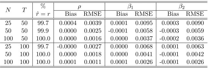
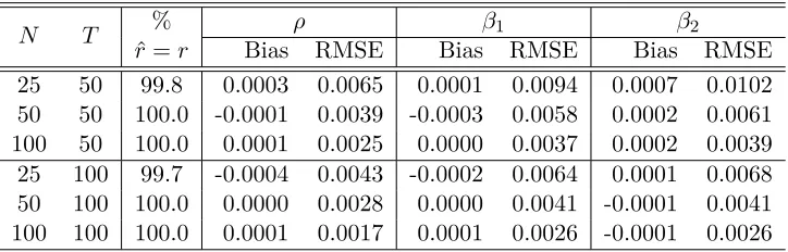
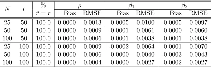
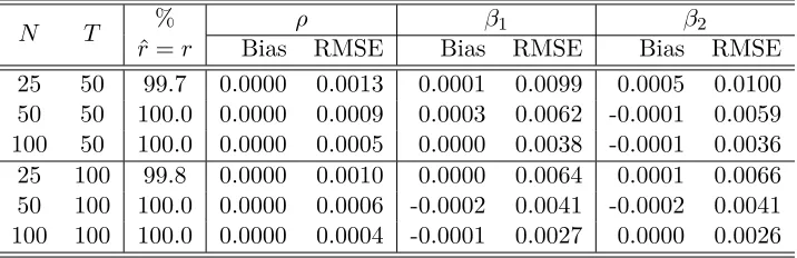
The following four tables present the simulation results which are obtained based on 1000 repetitions. Biases and root mean square errors (RMSE) are both computed. The percentage that the factor number is correctly estimated is given in the third column of each table. Different values ofρand different spatial weights matrices are considered. The tables show that the MLE has good finite sample properties. The number of factors can be correctly estimated with high probability. The biases are small. The RMSE of the estimators decreases as the sample becomes larger, indicating that they are consistent.

Table 1: The performance of the MLE underρ= 0.2 with “1 ahead and 1 behind” spatial weights matrix

N T %

ˆ r=r

ρ β1 β2

Bias RMSE Bias RMSE Bias RMSE 25 50 99.7 0.0004 0.0039 0.0001 0.0095 0.0003 0.0090 50 50 99.9 0.0000 0.0025 -0.0001 0.0058 -0.0003 0.0059 100 50 100.0 0.0000 0.0016 0.0000 0.0037 -0.0002 0.0036 25 100 99.7 -0.0000 0.0027 0.0000 0.0068 0.0001 0.0063 50 100 100.0 0.0000 0.0018 0.0000 0.0041 -0.0001 0.0042 100 100 100.0 0.0001 0.0011 0.0001 0.0026 -0.0001 0.0026

Table 2: The performance of the MLE underρ= 0.9 with “1 ahead and 1 behind” spatial weights matrix

N T %

ˆ r=r

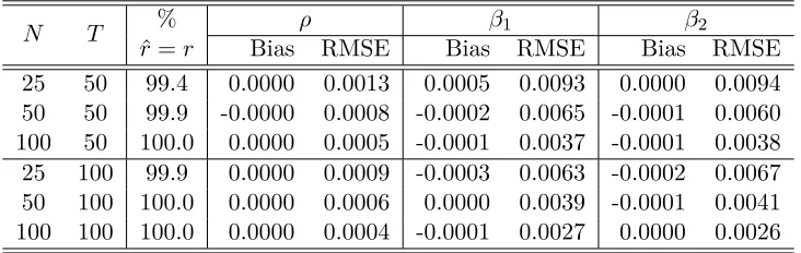
ρ β1 β2

Table 3: The performance of the MLE underρ= 0.2 with “3 ahead and 3 behind” spatial weights matrix

N T %

ˆ r=r

ρ β1 β2

Bias RMSE Bias RMSE Bias RMSE 25 50 99.3 -0.0002 0.0062 0.0004 0.0092 0.0004 0.0095 50 50 100.0 -0.0002 0.0037 -0.0001 0.0058 -0.0003 0.0057 100 50 100.0 0.0001 0.0025 -0.0001 0.0037 -0.0001 0.0037 25 100 100.0 -0.0002 0.0045 0.0001 0.0069 -0.0000 0.0067 50 100 100.0 0.0000 0.0028 0.0002 0.0040 0.0001 0.0040 100 100 100.0 0.0000 0.0017 -0.0001 0.0024 0.0000 0.0025

Table 4: The performance of the MLE underρ= 0.9 with “3 ahead and 3 behind” spatial weights matrix

N T %

ˆ r=r

ρ β1 β2

Bias RMSE Bias RMSE Bias RMSE 25 50 99.4 0.0000 0.0013 0.0005 0.0093 0.0000 0.0094 50 50 99.9 -0.0000 0.0008 -0.0002 0.0065 -0.0001 0.0060 100 50 100.0 0.0000 0.0005 -0.0001 0.0037 -0.0001 0.0038 25 100 99.9 0.0000 0.0009 -0.0003 0.0063 -0.0002 0.0067 50 100 100.0 0.0000 0.0006 0.0000 0.0039 -0.0001 0.0041 100 100 100.0 0.0000 0.0004 -0.0001 0.0027 0.0000 0.0026

7

Extensions

This section discusses two extensions: one allows time-invariant and common regressors, and the other allows a spatial autoregressive (SAR) specification for the errors. Both extensions are of practical relevance, and both can be studied within the ML framework.

7.1 Models with time-invariant and common regressors

Consider the following extended spatial panel data models with common shocks

yit=ρ N

X

j=1

wij,Nyjt+ k

X

p=1

xitpβp+r′iht+τi′pt+λ′ift+eit;

xitp =r′istp+ηip′ pt+γip′ ft+vitp; for p= 1,2, . . . , k.

(7.1)

whereri represents a vector of observable time-invariant variables such as race, gender, and

education;ptrepresents a vector of observable common variables (not varying withi) such

individual dependent. Imposing constant coefficients for these variables are also easy (Bai, 2009). Also note that we allow xit to be correlated with the time-invariant regressors ri

and with the common regressorspt, as shown in thex equation.

Model (7.1) falls within the framework of commons shocks. Letf_t†= (h′

t, p′t, s′t1, . . . , s′tk, ft′)′,

and let Φ†_i be defined as

Φ†_i =

"

r′

i τi′ 0 λ′i

0 η_i′ Ik⊗r′i γi′

#

whereηi = (ηi1, . . . , ηik) and γi= (γi1, . . . , γik). We can rewrite model (7.1) as

"

yit−ρPNj=1wij,Nyjt−Pkp=1xitpβp

xit

#

= Φ†_if_t†+ǫit,

which is similar to the model in Section 2. The difference here is that some components of the common factors f_t† are observable, and some components of the factor loadings Φ†_i are observable. The maximum likelihood method is good at imposing restrictions. The observed components off_t†and of Φ†_i are not estimated but are restricted to their observed values.

We will not pursue the asymptotic analysis for this model to conserve space. A related investigation is given in Bai and Li (2014) in the absence of spatial effects. Instead we run a small simulation to demonstrate the performance of the MLE. The data are gen-erated according to (7.1). The way to generate the factors, factor loadings, errors and heteroscedasticity is similar to Section 6. Other prespecified parameters are also the same except ρ = 0.5. The spatial weights matrix is that of “3 ahead and 3 behind.” The di-mensions of ft, ht and pt are all one. We do not report the estimated coefficients for the

time-invariant regressor and the common regressor (ri, pt) (there are many of them). For

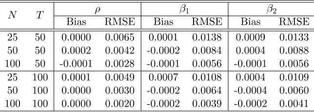
simplicity, we assume that the number of factors is known (it can also be estimated easily). Table 5 reports the simulation results based on 1000 repetitions. It is seen that the MLE performs quite well in the presence of time-invariant and common regressors.

Table 5: The performance of the MLE

in the presence of time-invariant and common regressors

N T ρ β1 β2

Bias RMSE Bias RMSE Bias RMSE 25 50 0.0000 0.0065 0.0001 0.0138 0.0009 0.0133 50 50 0.0002 0.0042 -0.0002 0.0084 0.0004 0.0088 100 50 -0.0001 0.0028 -0.0001 0.0056 -0.0001 0.0056 25 100 0.0001 0.0049 0.0007 0.0108 0.0004 0.0109 50 100 0.0000 0.0030 -0.0002 0.0064 -0.0004 0.0060 100 100 0.0000 0.0020 -0.0002 0.0039 -0.0002 0.0041

7.2 SAR disturbances

(2003), Baltagi et al. (2007), Kapoor et al. (2007), and Lee and Yu (2010). Here we consider spatial effects both in the dependent variable and in the errors, together with common shocks. Consider the following model

Yt=α+ρWNYt+Xtβ+ Λft+Ut (7.2)

with Ut = πMNUt+et, where MN is another spatial weights matrix with its diagonal

elements being zeros; Yt,α, andUt areN ×1 vectors, Xt isN ×k, and Λ = (λ1, ..., λN)′.

If the common shock term Λft does not exist, the preceding model reduces to that of Lee

and Yu (2010); but again we allow cross sectional heteroskedasticity.

To render an expression consistent with model (1.1), premultiply IN −πMN on both

sides. Then

Yt= (α−πMNα)+ρWNYt+πMNYt−ρπMNWNYt+Xtβ−πMNXtβ+(Λ−πMNΛ)ft+et.

We can treat α₋πMNα as a new α and Λ−πMNΛ as a new Λ since they are free

parameters. Now the above equation can be written as

Yt=α+ρWNYt+πMNYt−ρπMNWNYt+Xtβ−πMNXtβ+ Λft+et,

which can be alternatively written as

yit =αi+ρ

XN

j=1

wij,Nyjt

+π

N

X

j=1

mij,Nyjt

−ρπ

N

X

j=1

N

X

l=1

mij,Nwjl,Nylt

+x′_itβ₋π

N

X

j=1

mij,Nx′jt

β+λ′_ift+eit

(7.3)

wherewij,N and mij,N are the elements ofWN andMN. Similar to model (1.1), we allow

the regressors also to be affected by the common shocks,

xit=νi+γi′ft+vit. (7.4)

Combining (7.3) and (7.4), by the same method in Section 2, we can rewrite the model as

D(ρ, β, π)zt=µ+ Φft+ǫt (7.5)

whereµ, Φ andǫtare defined in the same way as in Section 2;D(ρ, β, π) is anN(k+ 1)×

N(k+ 1) matrix, whose (i, j) subblock, denoted by Dij(ρ, β, π), is equal to

Dij(ρ, β, π) =

            

"

1 +ρπmi∗,Nw∗i,N −β′

0 Ik

#

if i=j

"

−ρwij,N −πmij,N +ρπmi∗,Nw∗j,N πmij,Nβ′

0 0

#

if i₆=j

Model (7.5) is similar to (2.2) except that the transformation matrix D is more com-plicated. Nevertheless, the inverse matrix of D(ρ, β, π), denoted by V(ρ, β, π), still has a closed form. LetVij(ρ, β, π) be the (i, j)th subblocks of V(ρ, β, π), then we have

Vij(ρ, β, π) =

            

"

[(IN −πMN)(IN −ρWN)]ii (IN −ρWN)iiβ′

0 Ik

#

if i=j

"

[(IN−πMN)(IN −ρWN)]ij (IN −ρWN)ijβ′

0 0

#

if i₆=j

where [(IN −πMN)(IN −ρWN)]ij and (IN −ρWN)ij are the respective (i, j)th elements

of [(IN−πMN)(IN−ρWN)]−1 and (IN−ρWN)−1. Using the above result, the analysis of

the MLE is similar as model (1.1).

We use simulations to illustrate the performance of the MLE. The data are generated according to (7.5). The factors, factor loadings, errors and heteroskedasticity are generated in the same way as in Section 6. Other prespecified parameters such as the number of factors, the number of regressors and the true values ofβ are also the same; we setρ= 0.5 andπ= 0.4;WN andMN are set equal to each other and to be the “3 ahead and 3 behind”

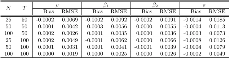
weights matrix. For simplicity, the number of factors is assumed to be known. Table 6 reports the simulation results based on 1000 repetitions.

Table 6 shows that the maximum likelihood method continue to perform well. The RMSE decreases as the sample size becomes larger, implying that the MLE is consistent.

Table 6: The performance of the MLE under SAR disturbances

N T ρ β1 β2 π

Bias RMSE Bias RMSE Bias RMSE Bias RMSE 25 50 -0.0002 0.0069 -0.0002 0.0092 -0.0002 0.0091 -0.0014 0.0185 50 50 0.0001 0.0042 0.0003 0.0056 0.0000 0.0055 -0.0004 0.0113 100 50 0.0002 0.0026 0.0001 0.0035 0.0000 0.0036 -0.0003 0.0073 25 100 0.0002 0.0049 -0.0001 0.0062 0.0000 0.0066 -0.0008 0.0126 50 100 0.0001 0.0031 0.0001 0.0041 -0.0001 0.0039 -0.0004 0.0079 100 100 0.0000 0.0019 0.0000 0.0025 0.0000 0.0026 -0.0002 0.0049

A further extension is to consider spatial weights on the lag Yt−1. The idea of joint

modeling of spatial effects and common shocks is similar and the MLE is still applicable.

8

Conclusion

References

Ahn, S. G., Lee, Y. H. and Schmidt, P. (2013): Panel data models with multiple time-varying effects,Journal of Econometrics, 174, 1-14.

Anderson, T.W. (2003). Introduction to Multivariate Statistical Analysis. Hoboken, New Jersey: John Wiley & Sons.

Anselin, L. (1988). Spatial econometrics: methods and models. The Netherlands: Kluwer Academic Publishers.

Bai, J. (2009) Panel data models with interactive fixed effects.Econometrica, 77(4), 1229– 1279.

Bai, J. and Li, K. (2012) Statistical analysis of factor models of high dimension,The Annals of Statistics, 40(1), 436–465.

Bai, J. and Li, K. (2014) Theory and methods of panel data models with interactive effects,

The Annals of Statistics, 42(1), 142–170.

Baltagi, B., Song, S.H., and Koh, W. (2003) Testing panel data regression models with spatial error correlation,Journal of Econometrics, 117, 123-150.

Baltagi, B., Song, S.H., Jung, B.C., and Koh, W. (2007) Testing for serial correlation, spatial autocorrelation and random effects using panel data, Journal of Econometrics, 140, 5-51.

Case, A. C. (1991) Spatial patterns in household demand.Econometrica, 59(4), 953–965.

Case, A. C., Rosen, H. S., and Hines, J. R. (1993) Budget spillovers and fiscal policy interdependence: Evidence from the states. Journal of Public Economics, 52(3), 285-307.

Chamberlain, G. and Rothschild, M. (1983): Arbitrage, factor structure, and mean-variance analysis on large asset markets,Econometrica,51:5, 1281–1304.

Cliff, A. D., and Ord, J. K. (1973) Spatial autocorrelation, London: Pion Ltd.

Conley, T. G. (1999). GMM Estimation with Cross Sectional Dependence, Journal of Econometrics, 92, 1-45.

Conley, T.G., and Dupor, B. (2003) “A Spatial Analysis of Sectoral Complementarity,” Journal of Political Economy, 111, 311-352.

Cressie, N. (1993): Statistics for Spatial Data. New York: John Wiley & Sons.

Dempster, A. P., Laird, N. M., and Rubin, D. B. (1977). Maximum likelihood from in-complete data via the EM algorithm.Journal of the Royal Statistical Society. Series B (Methodological), 1-38.

Glaeser, E. L., Sacerdote, B., and Scheinkman, J. A. (1996) Crime and social interactions.

Jennrich, R. I. (1969) Asymptotic properties of non-linear least squares estimators. The Annals of Mathematical Statistics, 40(2), 633-643.

Kapoor, M., Kelejian, H. H., and Prucha, I. R. (2007). Panel data models with spatially correlated error components.Journal of Econometrics, 140(1), 97-130.

Kelejian, H. H., and Prucha, I. R. (1998) A generalized spatial two-stage least squares procedure for estimating a spatial autoregressive model with autoregressive disturbances.

The Journal of Real Estate Finance and Economics, 17(1), 99-121.

Kelejian, H. H., and Prucha, I. R. (1999) A generalized moments estimator for the autore-gressive parameter in a spatial model.International economic review, 40(2), 509-533.

Kelejian, H. H., and Prucha, I. R. (2010). Specification and estimation of spatial autore-gressive models with autoreautore-gressive and heteroskedastic disturbances.Journal of Econo-metrics, 157(1), 53-67.

Lee, L. (2004a) Asymptotic distribution of quasi-maximum likelihood estiators for spatial augoregressive models,Econometrica, 72(6), 1899–1925.

Lee, L. (2004b) A supplement to “Asymptotic distribution of quasi-maximum likelihood estiators for spatial augoregressive models”, Manuscipt.

Lee, L. and Yu, J. (2010) Estimation of spatial autoregressive panel data models with fixed effects,Journal of Econometrics, 154(2), 165-185.

Lin, X., and Lee, L. F. (2010) GMM estimation of spatial autoregressive models with unknown heteroskedasticity.Journal of Econometrics, 157(1), 34-52.

Liu, C., and Rubin, D. B. (1994) The ECME algorithm: a simple extension of EM and ECM with faster monotone convergence.Biometrika, 81(4), 633-648.

McLachlan, G. J., and Krishnan, T.The EM Algorithm and Extensions. 1997. New York: Wiley

Moon, H. and Weidner, M. (2009): Likelihood expansion for panel regression models with factors, manuscipt, University of Southern California.

Newey, W.andMcFadden, D. (1994): Large Sample Estimation and Hypothesis Test-ing, in Engle, R.F. and D. McFadden (eds.)Handbook of Econometrics, North Holland.

Ord, K. (1975). Estimation methods for models of spatial interaction. Journal of the Amer-ican Statistical Association, 70(349), 120-126.

Pesaran, M. H. (2006) Estimation and inference in large heterogeneous panels with a multifactor error structure, Econometrica, 74(4), 967–1012.

Pesaran, M. H., and Tosetti, E. (2011). Large panels with spatial correlations and common factors, Journal of Econometrics, 161, 182–202.

Stock, J. H., and Watson, M. W. (1998). Diffusion indexes (No. w6702).National Bureau of Economic Research.

Topa, G. (2001). Social Interactions, Local Spillovers and Unemployment,Review of Eco-nomic Studies, 68, 261-295.

Appendix: Proofs for the theorems in the main text

In the appendix, we provide the detailed proofs for the theorems in the main text. We first define some notations which will be used throughout the appendix.

ˆ

H= ( ˆΦ′Σˆ−_ǫǫ1Φ)ˆ −1; HˆN =N ·Hˆ;

ˆ

G= (Ir+ ˆΦ′Σˆ−ǫǫ1Φ)ˆ −1; GˆN =N ·G.ˆ

Appendix A: Proof for consistency

While in the main text, we use (ρ, β,Φ,Σǫǫ) to denote the true value of the coefficients.

For proving consistency, we shall use a superscript “*” to denote the true values of param-eters; the variables without “*” denote the input variables of the likelihood function. This notation is only used in Appendix A. Once consistency is established, we will drop “*” in Appendices B to F. The following lemmas are useful for the proof of consistency.

Lemma A.1 Let V(ρ, β) be the inverse matrix of D(ρ, β), then

Vij(ρ, β) =

            

"

(I₋ρWN)ii (I−ρWN)iiβ′

0 Ik

#

if i=j

"

(I₋ρWN)ij (I−ρWN)ijβ′

0 0

#

if i₆=j

(A.1)

where Vij(ρ, β) is the (i, j)th subblock of V and (I −ρWN)ij is the (i, j)th element of

(I ₋ρWN)−1. Furthermore, let R = (IN −ρWN)(IN −ρ∗WN)−1 and D = DD∗−1 with

D∗_=D(ρ∗_{, β}∗_{). We have}

D_{ij =}

            

"

Rii Riiβ∗′−β′

0 IK

#

if i=j

"

Rij Rijβ∗′

0 0

#

if i₆=j

where D_{ij is the (i, j)th subblock of} D_{and Rij is the (i, j)th element of R.}

Proof of Lemma A.1. This follows from direct verification.

Lemma A.2 Let(ρ, β)_{∈ A×B}, where_Aand_Bare both compact sets. Under Assumptions A-F, uniformly on_{A × B},

(a)

N

X

j=1

Rij(γj∗β∗+λ∗j)−γi∗′β