Munich Personal RePEc Archive
The debt trap: a two-compartment train
wreck...and how to avoid it
Artzrouni, Marc and Tramontana, Fabio
University of Pau, University of Pavia
2 October 2013
Online at
https://mpra.ub.uni-muenchen.de/50347/
The debt trap: a two-compartment train wreck...
and how to avoid it
Marc Artzrouni
Department of Mathematics (UMR CNRS 5142) and
Center for the Theoretical Analysis and Handling of Economic Data
University of Pau; FRANCE
Fabio Tramontana
Department of Economics and Management
University of Pavia; ITALY
20 September 2013
Abstract
We explore sustainable paths out of a debt trap with a highly stylized two-sector
differential equations model for the stocks of money in Government and Society. The
model fits the data for the U.S. between 1981 and 2012 with a coefficient of
corre-lation of 0.996. The solutions provide detailed “escape conditions” from the debt
trap. A primary surplus is required. Then a government can escape its debt trap
either through sustained annual monetary outflows from society to the government
(taxation) but with a low initial growth rate, or through annual monetary inflows
into both sectors (stimulus) with higher initial growth rate. We illustrate the use
of our model with simulations which show how five indebted countries can escape
their debt trap in 30 (or 70) years.
Keywords: Compartmental model, debt, system of differential equations, dynamical
sys-tem, fiscal policy.
JEL Classification: C51, C62, C63, E61, H63.
E-mail: [email protected]; [email protected]
1
Introduction
Many countries today have a debt to GDP ratio between 50 and 100 %. A few are above
100 % and Japan tops the chart well over 200 %. A debate rages between “hawks” who
advocate rapid deficit reduction and “doves” who believe the best way out of the debt
trap is to tax less and stimulate more (Cottarelli, 2013).
Those in the first group feel that debt-reduction is indeed the first priority. For
example Reinhart and Rogoff (2010) warn against a debt above 90% of GDP - a finding
questioned by some (Herndon et al., 2013). Those in the second group, led by Krugman
urge caution and warn that austerity can lead to doubts about government solvency
(see Krugman (2012) and other articles on Krugman’s blog). They also fear the
long-term impact of reduced growth associated with austerity measures and advocate stimulus
spending instead of austerity. One can see both sides: pro-austerity economists emphasize
the need to stabilize public finances while pro-stimulus ones fear that austerity can be a
vicious circle that keeps an economy permanently in its debt trap.
In their attempts at finding objective solutions to these fraught questions, policy
mod-ellers have deployed impressive arsenals of sophisticated mathematical tools that were
supposed to help policy-makers understand, predict and affect macroeconomic trends
(Ruiz Estrada and Yap, 2013). Perhaps the best-known of these tools are the Discrete
Stochastic General Equilibrium (DSGE) models. Although criticized by some (Solow,
2010; Kocherlakota, 2010; Knibbe, 2013) these models have proved useful and have
in-formed macro-economic debates. They are used by Central Banks and the European
Union among others (see Ratto et al. (2009), Marattin et al. (2011) and Annicchiarico
et al. (2013) for a recent application to Italy). For example Trachanas and Katrakilidis
(2013) warn of unsustainable debt in Greece, Italy, and Spain.
More generally econometric methods have been used to assess the role of taxation and
find ways of restoring “ fiscal sanity” (Hauptmeier et al., 2011; Saunoris and Payne, 2010).
Others have studied “fiscal gaps” in order to assess the fiscal consolidation required for an
Budget Office issues detailed budget projections (CBO, 2013). A highly stylized model
with a “good” and a “bad” equilibrium has been used to explore conditions under which
the southern euro area could move from one equilibrium to the other (Padoan et al.,
2013). This model relies on two variables (output Y and real government debt D). The
dynamics are formulated with a simple differential equation.
The model we propose here is similar in spirit to the good/bad equilibrium model of
Padoan et al. (2013): it is both extremely parsimonious (also two variables) and extremely
simple. Ours is a “toy model” which aims to shed light on the macroeconomic conditions
needed for an escape from the debt trap. We focus on the “very big picture”, that is the
flow of money in and out of government. Indeed, national governments are like households
and firms: money flows in, money flows out, and the balance contributes to the stock of
money in the system. A natural and simple way of describing these flows is with a
two-sector economy, Government (G) and Society (S), each one characterized by its stock
of money (money supply). Ours is a dynamical systems approach: accounting identities
are formulated through a system of two linear differential equations which capture the
essential mechanisms that drive the monetary flows between the two compartments. Such
a compartmental representation is borrowed from epidemiology and has been recently
introduced in economics (Tramontana, 2010).
In Section 2 we describe the model and provide simple closed-form expressions for the
two stocks. In Section 3 we show that the model captures well the trajectories of the
two stocks in the U.S. from 1981 to 2012. In Section 4 we formulate escape conditions
which show that an escape hinges on a fine balance between a primary surplus and the
inflows into (or between) the two compartments. In Section 5 we apply the model by
showing how five indebted countries can theoretically escape their debt trap in 30 (or
70) years. Section 6 discusses policy prescriptions and perspectives while Section 7 closes
2
The model
A compartmental representation is used to describe a two-sector economy consisting of a
Government and Society. The G and S compartments are characterized at every instant
t by the stocks of money G(t) and S(t) in the two sectors (Figure 1). In the sequel a
compartment’s ”stock” will always refer to its stock of money.
Government G(t)
Society S(t)>0
s S(t)
-i G(t)
i S(t)
aG aS
[image:5.595.126.380.223.389.2]Central and other banks
Figure 1: Compartmental model of Government and Society stocks with links to Central and other banks. If a flow is given as a positive value it is in the direction of the arrow, and
vice versa. For example if the government stock G(t) is negative the interest flow −ιG(t)
is positive and in the direction of the arrow, towards the banks. If G(t) escapes the debt
trap and becomes positive the flow −ιG(t) is negative and in the opposite direction to the
arrow, towards G. Bidirectional arrows reflect our uncertainty concerning the direction of the annual flows that are needed for an escape from the debt trap.
The model is in continuous time and we will describe the temporal dynamics of G(t)
and S(t) in nominal terms with a system of two linear differential equations:
dG
dt =
monetary policy
z }| {
ιG+αG +
fiscal policy
z}|{
σS (1)
dS
dt = ιS+αS − σS. (2)
The first components of the derivatives are the interests ιG(t) and ιS(t) that are
received or paid out depending on the sign of G(t) and S(t). A simplification of the
interest rate” ι. When G(t) is negative then ιG(t) is negative and is an interest paid.
With S(t) being positive the S compartment earns an interest ιS(t) per unit of time.
These interest flows link the G and S compartments to an outside world of banks and
other financial institutions that lend, borrow and print money. (For this reason these
financial institutions must not be included in the S sector).
The constant annual flows αG and αS are of arbitrary sign. A positive α reflects an
infusion of “fresh money” resulting from money printing, quantitative easing, government
bond-buying, a positive balance of trade, etc. A negative α reflects annual expenditures
which can benefit the other compartment, e.g. constant annual expenditures/stimulus
from G to S or constant tax flow from S to G (more on this in the discussions). The
“monetary policy” annotation in Eqs. (1) - (2) reflects the role of the interest rate ι and
of the annual monetary flows αG and αS.
The quantity σS(t) is a net annual flow from S into G. This flow captures the
bal-ance of receipts (e.g. taxes) and of outlays (e.g. schools, civil servants, defense, etc.).
These receipts and outlays are assumed to be intrinsically proportional to the size of the
economy/population crudely measured by society’s stock S(t). The coefficient of
pro-portionality σ (or ”transfer rate”) is positive when receipts exceed outlays and negative
otherwise (always assumingS(t) remains positive). The “fiscal policy” annotation in Eqs.
(1) - (2) reflects the role of taxation and government spending which are captured in the
transfer rate σ.
In short the government and society’s stocks both change under three effects: i) a
constant flow in or out of each compartment (the α’s); ii) interests paid or received at
rate ι; iii) a primary surplus or deficit at rateσ (i.e. the net transfer σS(t) of government
funds in or out of the S compartment, which excludes interest payments).
S alone. The solution is
G(t) = (ι(G(0) +S(0)) +αG+αS)
eιt
ι −
S(0) + αS
ι−σ
e(ι−σ)t+σ(αG+αS)−ιαG
ι(ι−σ) ,
(3)
S(t) =
S(0) + αS
ι−σ
e(ι−σ)t− αS
ι−σ. (4)
3
Model fitting to U.S. data
We illustrate the model with data on the total (federal) public debt in the U.S. (G(t))
which is readily available. We recognize that this is gross simplification, mostly because
we ignore the role of states which provide many services. Society’s stock is an even bigger
challenge. The money supplies M1-M3 come to mind but we are unsure which one is the
most relevant; M1 or M3 may be too narrowly or broadly defined. In the U.S. no data on
the M3 money supply is available after 1986. For these reasons we chose M2.1
We fit the model starting in 1981, the earliest year available for the readily
download-able data on M2 from the Federal Reserve.2 The last data point was for 2012 (n = 32).
We fixed the initial values of the stocks G(0) andS(0) at their 1981 values.
We next need at least a crude estimate for a constant value of our ”intrinsic interest
rate” ι during the period 1981-2012. We divided for each year the ”Interest Expense on
National Debt” by the debt as a naive estimate of the interest rate paid by the government.
This interest rate declined from roughly 7 to 4 % during the 32 years between 1981 and
2012. We thus chose to estimate ι as the average value during that period which is
ι= 5.875%.
1
If society’s real stock is quite different from M2 and/or immeasurable this complicates the use of the model, although all is not necessarily lost. Indeed suppose a ”real” stock S were an affine but unknown function of the M2 stock: S = ρ0+ρ1M2. Substituting this expression for S in Eqs. (1)-(2) yields a
model in (G(t), M2(t)) that is structurally the same as before with M2(t) as a proxy stock for society. Indeedσ becomes ρ1σ; αG becomes αG+ρ0σ and αS becomes αS−ρ0σ. The unknownρ’s have been
folded into the model’s unknown parameters.
2
Estimates Value c
αG -0.07447
c
αS -0.02359
b
σ -0.00561
[image:8.595.225.373.67.145.2]Coeff. corr. r 0.996
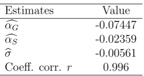
Table 1: Parameter estimates and coefficient of correlation in fitting of U.S. data (1981-2012).
With ι now fixed we define the vector θ of the three remaining parameters
θ= (αG, αS, σ). (5)
The parameters are estimated by minimizing over θ the sum of squared deviations
SS1(θ) =
X
k
(G(k)actual−G(k, θ))2+X
k
(S(k)actual−S(k, θ))2 (6)
where G(k, θ) and S(k, θ) are for the year k the modelled values given in Eqs. (3)-(4).
The initial values of the stocks are the debt and M2 money supply on 1/1/1981: G(0) =
−0.991;S(0) = 1.679 (in trillions of USD). Standard numerical procedures converged
nicely to the same estimated value bθ = (αcG,αcS,σ) for any reasonable initial values ofb
the parameters. The three parameter estimates are given in Table 1 together with the
coefficient of correlation.3
The solutions in Eqs. (3)-(4) are now
G(t) = −0.98105 e0.05875t−1.31213 e0.06437t+1.3026 (7)
S(t) = 1.31213 e0.06437t+0.36657 (8)
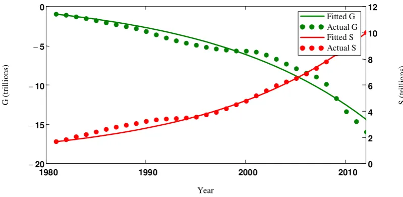
with t = 0 corresponding to Jan 1, 1981 (Figure 2). With a coefficient of correlation of
0.996 the model is able to describe with four parameters (one of which, ι, was fixed) the
3
dynamics of the U.S. debt and of the M2 stock of money over 32 years.
Equation (7) shows unsurprisingly that the U.S. economy is caught in a debt trap:
extrapolating the model beyond 2012 leads to an irreversible decline of the government
stock, which is neither desirable nor realistic. In the next section we will find what
parameter values can reverse such a trend and bring an indebted government’s stock back
into positive territory.
1980 1990 2000 2010
20
-15
-10
-5
-0
0 2 4 6 8 10 12
Fitted G Actual G Fitted S Actual S
Year
G
(
tr
il
li
ons
)
S
(
tr
il
li
o
ns
[image:9.595.111.511.246.441.2])
Figure 2: Fitted and actual trajectories of public debt G (left axis) and M2 money supply S (right axis) in the U.S., 1981-2012, trillions of USD (coefficient of correlationr= 0.996).
4
Dimensionless dynamics and escape conditions
4.1
Dimensionless dynamics
The public debt and the deficit are usually measured as percentages of GDP in order
to make international comparisons with dimensionless quantities that do not depend on
monetary units. We do the same here by defining the stocks of the two compartments as
fractionsG∗(t) and S∗(t) of theinitial gross domestic productGDP(0) =v(0)S(0) where
and the five countries below):
G∗(t)def.= G(t)
GDP(0) =
G(t)
v(0)S(0), (9)
S∗(t)def.= S(t)
GDP(0) =
S(t)
v(0)S(0). (10)
In a similar manner we define the model’s annual inflows into the two compartments as
fractions of initial GDP:
α∗
G
def.
= αG/GDP(0);α∗S
def.
= αS/GDP(0). (11)
With these notations the solutions are the starred equivalents of Eqs. (3)-(4), namely
G∗(t) = (ι(G∗(0) +S∗(0)) +α∗
G+α∗S)
eιt
ι −
S∗(0) + α
∗
S
ι−σ
e(ι−σ)t+σ(α ∗
G+α∗S)−ια∗G
ι(ι−σ) ,
(12)
S∗(t) =
S∗(0) + α
∗
S
ι−σ
e(ι−σ)t− α ∗
S
ι−σ. (13)
The initial conditions are now the initial debt to GDP ratio G∗(0) = G(0)/GDP(0) and
the inverse of the initial velocity of money S∗(0) = S(0)/GDP(0) = 1/v(0), two readily
available statistics for most countries.
4.2
Escape conditions
We will say that the economy escapes the debt trap if in the long-run both G∗(t) and
S∗(t) remain positive. Equations (3)-(4) show that this can only happen with G∗(t) and
S∗(t) in the long run growing exponentially with rates ι >0 and ι−σ > 0 respectively
(i.e. G∗(t) ∼ eιt and S∗(t) ∼ e(ι−σ)t for large t). Before giving the escape conditions in
the proposition below we define
ωG
def.
= −ιG∗(0)−σS∗(0), ω
S
def.
and
tm
def. =
ln α∗S+S∗(0)(ι−σ) α∗
G+α∗S+ι(G∗(0)+S∗(0))
σ if argument of ln is >1, (15a)
0 otherwise, (15b)
where tm of Eq. (15a) is the root of the equation dG∗(t)/dt = 0 (from Eq. (12)) when
the argument of the logarithm is larger than 1; G∗(t) then reaches an extremum at t
m.
Proposition 1. Given initial conditions G∗(0) and S∗(0) we define condition C1 as
0 < σ < ι. The conditions for the asymptotic exponential growths of G∗(t) and S∗(t)
are:
C2(for G∗(t)∼eιt) : α∗
G+α∗S >−ι(G∗(0) +S∗(0)) =ωG+ωS, (16)
C3(for S∗(t)∼e(ι−σ)t) : α∗
S > S∗(0)(σ−ι) =ωS <0. (17)
If in addition to C1-C3 the condition
C4(for dG∗(0)/dt >0) : α∗
G>−ιG∗(0)−σS∗(0) =ωG (18)
is also satisfied then the government stock G∗(t)starts increasing immediately and
mono-tonically. In this case the argument of the logarithm in Eq. (15a) is ≤ 1 and we have
a “Rapid Escape” with a “time of minimum” tm equal to 0 (Eq. (15b)). If C4 is not
satisfied then the argument of the logarithm is >1; G∗(t) begins by decreasing to reach a
minimum at time tm in Eq. (15a) and then increases exponentially without bounds - we
have a “Delayed Escape”.
Proof. Equation (4) shows that both ι−σ andS(0) +αS/(ι−σ) must be positive
(condi-tions C1, C3) in order to have S(t)∼e(ι−σ)t. Equation (3) shows that we need 0 < σ < ι
and ι(G(0) +S(0)) +αG+αS >0 (C1, C2) in order to have G∗(t)∼eιt. Under condition
C4 the stock G∗(t) initially increases and this increase can only be monotone. If C4 is
a minimum that can only by at time tm of Eq. (15a). Then G∗(t) increases without
bounds.
s = - l Rapid Escape
(C1-C4: 𝑮 ↑, 𝑺 ↑)
l=[a
i
Delayed Escape (C1-C3, not C4:
𝑮 ∪, 𝑺 ↑))
(𝑮 ↓, 𝑺 ↑)
No Escape
a𝑺∗
a𝑮∗
(w w )
(wG ,wS)
wG + wS
𝑮 ↑, 𝑺 ↓
s
𝝎𝑺= 𝝈−𝜾𝒗 < 0
𝝎𝑺=𝝈 − 𝜾𝒗
𝛔
𝛊
No Escape
Delayed Escape (C1-C3, not C4:
𝑮 ∪, 𝑺 ↑)) Rapid Escape
(C1-C4: 𝑮 ↑, 𝑺 ↑)
No Escape C4 C4 C2 C2 C3 C3 C1 Escape conditions:
a) in (a𝑮∗,a𝑺∗) space
[image:12.595.100.342.142.465.2]b) in (𝜾, 𝝈) space
Figure 3: Typical escape conditions in the (α∗
G, α∗S) space and in the (ι, σ) space. Each
one of the straight-line conditions C1-C4 is plotted with the same color in both spaces (no visible C1 in (α∗
G, α∗S)). The rapid escape region is between the blue and green lines.
The critical case of both stocks remaining constant arises at the intersection of all three constraints C2-C4 (red, green and blue line).
In Figure 3 we plotted typical escape conditions/regions in the (α∗
G, α∗S) space (with
ι and σ assumed fixed and 0 < σ < ι) and in the (ι, σ) space (with α∗
G and α∗S assumed
fixed). Although the plots depend somewhat on the values of the fixed parameters Figure
3a shows that an escape hinges on a sufficiently large sum of annual flow (red
condi-tion/constraint C2 at a 45o angle). A rapid escape requires each flow to be larger than a
certain minimum (C3 (blue), C4 (green)). Figure 3b sheds light on the roles of ι and σ.
In this example α∗
S is assumed negative and a rapid escape hinges on the pair (ι, σ) being
4.3
Parameterization of escape
Given initial conditions G∗(0) andS∗(0) we want to explore realistic parameter values for
which an escape can occur. Once we have chosen an interest rate ιand a positive transfer
rate σ < ι we need to choose annual flows α∗
G and αS∗ in the delayed or rapid escape
regions given in Figure 3. We will see in the Applications section that even countries
that are considered seriously indebted can have negative sumsωG+ωS, meaning that the
initial debt |G(0)| is less than society’s initial stock of money S(0) (as in Figure 3). In
this case zero flowsα∗
G and α∗S bring about at least a delayed escape since then conditions
C1-C3 are satisfied. However this would be of little use if it takes 50 years for G(t) to
reach its minimum or 200 years for G(t) to become positive.
For this reason we parametrize the annual flows required for an escape with two
economically meaningful parameters that specify the timing and tempo of the escape.
The first is the time until the escape te defined by G∗(te) = 0. Equation (12) shows that
te is the root of the equation
0 = (ι(G∗(0) +S∗(0)) +α∗
G+α∗S)
eιte
ι −
S∗(0) + α
∗
S
ι−σ
e(ι−σ)te
+σ(α
∗
G+α∗S)−ια∗G
ι(ι−σ) .
(19)
Although a root can always be found numerically, there is no closed form solution for te.
However with a specified escape time te Eq. (19) can be viewed as a linear constraint
between the two flows α∗
G and α∗S. This “iso-te” constraint will therefore find a straight
line expression in the (α∗
G, α∗S) space of Figure 4 (solid red lines). In order to decide which
point on the line to choose, we define a second parameter, namely the initial growth rate
γ of society’s stock, i.e.
γ def.= dS(0)/dt
S(0) =ι−σ+
α∗
S
S∗(0). (20)
We recall that GDP(t) = v(t)S(t). If the velocity of money v(t) remains constant and
equal to its initial value v(0) (at least for a short initial period) then GDP(t), S(t) and
S∗(t) are multiples of one another during that period. This means that the initial growth
an initial value of the growth rate of the GDP, which is a meaningful economic variable.
Equation (20) determines α∗
S as an affine function α∗S(γ) of γ >0:
α∗
S(γ)
def.
= (γ+σ−ι)S∗(0). (21)
We use Eqs. (19)-(21) to express α∗
G as an affine function α∗G(γ, te) ofγ:
α∗
G(γ, te)
def.
= γS∗(0)(σ−ιe
te(ι−σ)+ eιte(ι−σ))
(ι−σ)(1−eιte) −σS
∗(0) + ιe
ιteG∗(0)
1−eιte . (22)
Equations (21)-(22) define parametrically (with parameter γ) a straight-line “iso-te”
locus of values (α∗
G(γ, te), αS∗(γ)) for which the time of escape iste(solid red lines of Figure
4 for three values ofte). Specifying a small te, sayte= 1, and some desired initial growth
rateγ yields valuesα∗
G(γ,1) andα∗S(γ) which bring about an escape in one year. However
if the debt is severe the resulting α∗
G(γ,1) would be unrealistically large. The challenge
is to find a time of escape te that yields realistic annual flows α∗G(γ, te) and α∗S(γ). (Note
however that the flow α∗
S(γ) (Eq. (21)) in (or out of) S does not depend on te).
With an initial growth rateγ equal to 0 the point (α∗
G(0, te), α∗S(0)) is at the bottom
of the “iso-te” line, at the intersection with the blue horizontal borderline. Asγ increases
the point (α∗
G(γ, te), αS∗(γ)) travels up on the straight line and crosses the border between
the rapid and delayed escape regions at a value γ∗(t
e)4.
The slope of the “iso-te” line does not depend on initial conditions G∗(0) and S∗(0).
This means that the “iso-te” lines obtained in the Application section below for different
countries and common values of ι, σ and te will be parallel.
4
s = - l
Rapid Escape
l=[a
i
Delayed Escape
(𝑮 ↓, 𝑺 ↑)
a𝑺∗
a𝑮∗
(w w )
(wG ,wS)
wG + wS
𝑮 ↑, 𝑺 ↓
s
𝝎𝑺 =𝝈−𝜾𝒗 < 0
𝝎𝑺=𝝈 − 𝜾𝒗
Red straight-line loci (a𝑮∗ 𝜸, 𝒕𝒆 , a𝑺∗ 𝜸) of annual flows for fixed escape time 𝒕𝒆, parameterized by initial growth rate g 0.
g =0, tm 𝜸, 𝒕𝒆 =0
tm 𝜸, 𝒕𝒆 increases as g increases beyond g *(te)
No Escape g =g *(te),
tm 𝜸, 𝒕𝒆=0
g = i-s
C4
C2
C3
Smaller te
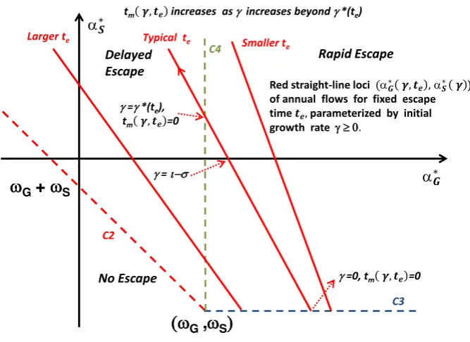
[image:15.595.117.451.121.364.2]Larger te Typical te
Figure 4: Space of annual flows (α∗
G, α∗S) with three red straight-line “iso-te” loci of flows
(α∗
G(γ, te), α∗S(γ)) needed forG(t) to becomes positive at timete (three different values of
te). A smaller escape time te requires larger annual inflowsαG∗(γ, te) into G. As the value
of the initial growth rate γ (which parametrizes the “iso-te” line) increases from 0 the
point (α∗
G(γ, te), α∗S(γ)) moves up the line starting at the horizontal blue borderline (see
“Typical te” red line). The time tm(γ, te) at which the G stock reaches its minimum is
zero as long as (α∗
G(γ, te), αS∗(γ)) is in the rapid escape region (Eq.(23b)); tm(γ, te) starts
increasing (Eq.(23a)) when (α∗
G(γ, te), α∗S(γ)) enters the delayed escape region, i.e. for
γ > γ∗(t
e).
When an economy is in debt (G∗(0) <0) the “iso-t
e” line always intersects the blue
C3 horizontal borderline on the right of the point (ωG, ωS) as in Figure 4. A shorter
escape time te means an “iso-te” line shifted/rotated to the right with a steeper negative
slope: the escape requires larger annual inflows into G. Conversely, a longer escape time
shifts/rotates the line to the left with a slope that is less steep but always < −1: more
time for an escape requires smaller annual inflows.
(15), can now be written as
tm(γ, te)
def. =
ln α∗S(γ)+S∗(0)(ι−σ) α∗
G(γ,te)+α∗S(γ)+ι(G∗(0)+S∗(0))
σ if argument of ln is > 1, (23a)
0 otherwise. (23b)
Equation (23b) (or Eq. (23a)) applies when (α∗
G(γ, te), α∗S(γ)) is in the rapid (or delayed)
escape region. In the next section we illustrate the model with projection scenarios that
show how five countries can escape their debt traps.
5
Appplication
We apply the model to five countries in various states of indebtedness with the initial time
set in 2011. The World Bank database provides the (initial) debt to GDP ratio G∗(0),
which is routine. They also provide the ratio of the M2 money supply (“quasi money”)
to GDP. Conveniently this is our S∗(0) = 1/v(0) with the M2 definition we chose for the
money supply. (Data in Table 2 with countries listed in increasing order of initial debt to
GDP ratio).
We set ι= 0.05, a plausible interest rate for our illustrative purpose. The parameter
σ is trickier and of course vital since an escape hinges on a positive value of σ. Our only
indication on its value is provided by the data fitting exercise for the U.S. which yielded
b
σ = −0.00561, a value pretty close to being positive. For this reason we somewhat
arbitrarily choose σ = 0.01, which combined with ι = 0.05 and a realistic escape time
te = 30 will provide plausible parameters and trajectories. (A smaller te would require
implausibly high annual inflows).
The big picture is given in Figure 5 where we have plotted the five “iso-te” segments
(te=30) parametrized by values of γ ranging from 0.02 to 0.04 and to 0.06. Based on
past experience these values represent a plausible range of initial growth rates (Salvatore,
2010). The dotted lines at a right angle are for each country the borders C3 and C4 of
the rapid escape region. Numerical values α∗
γ = 0.02,0.04,0.06.
In order to gauge however crudely the plausibility of the results for theα’s in Table 2
we can compare their maximum 0.071 (7.1 %) to the planned one-off injection of $ 0.475
trillion USD in the U.S. economy in 2008 (known as TARP for Troubled Asset Relief
Program). This amount was roughly 3 % of the year’s GDP. This was a one-off program
(actually spread over a couple of years) that was considered massive and we are talking
here of annual inflows continuing over decades. Still our percentages in the 0 to 7.1 %
range seem plausible for the purpose of our illustrative examples.
With a low initial growth rate of γ = 0.02 the escape occurs with annual outflows
α∗
S(0.02) between -1.7 % for Sweden and -3.2 % for France. When the absolute values of
these outflows are smaller than the corresponding flow α∗
G(30,0.02) into G these outflows
can be channelled into G and viewed as annual constant “adjustment” taxes. This reduces
the requirement for fresh funds into G accordingly. For example if γ = 0.02 then in the
U.S. an escape in 30 years is achieved with a (constant) diversion of |α∗
S(0.02)| = 1.8%
of initial GDP from S to G. The inflow of fresh funds into G is reduced from 4.1 %
to 2.3% which is the (algebraic) sum of flows α∗
G(30,0.02) +α∗S(0.02). In order for this
interpretation of the flows to be valid this sum of flows must be positive. However this
will always be the case with a sufficiently small te - which we are seeking anyway. (The
negative value -0.004 of the sumα∗
G(30,0.02) +α∗S(0.02) for Sweden withγ = 0.02 means
that the country could escape the debt trap in less than 30 years with a realistic net sum
of incoming flows just larger than 0).
The intermediate initial growth rateγ = 0.04 corresponds to the special caseγ =ι−σ.
The α∗
S(0.04) flows are then 0 for all countries. The corresponding flows α∗G(0.04,30) of
fresh money into the government sector range from 1% of initial GDP in the least indebted
Sweden U.S. France Greece Italy Initial conditions
G∗(0) = G(0)
GDP(0) -0.383 -0.818 -0.937 -1.065 -1.109
S∗(0) = 1
v(0) 0.867 0.897 1.585 0.979 1.538
ω’s
ωG 0.010 0.032 0.031 0.043 0.040
ωS -0.035 -0.036 -0.063 -0.039 -0.062
ωG+ωS -0.024 -0.004 -0.032 0.004 -0.021
γ=0.02
α∗
G(30,0.02) 0.013 0.041 0.039 0.055 0.051
α∗
S(0.02) -0.017 -0.018 -0.032 -0.020 -0.031
α∗
G(30,0.02) +α∗S(0.02) -0.004 0.023 0.007 0.036 0.020
γ =0.04
α∗
G(30,0.04) 0.010 0.038 0.034 0.052 0.046
α∗
S(0.04) 0 0 0 0 0
α∗
G(30,0.04) +α∗S(0.04) 0.010 0.038 0.034 0.052 0.046
γ=0.06
α∗
G(30,0.06) 0.007 0.035 0.029 0.049 0.041
α∗
S(0.06) 0.017 0.018 0.032 0.020 0.031
α∗
[image:18.595.118.478.70.373.2]G(30,0.06) +α∗S(0.06) 0.025 0.053 0.06 0.069 0.071
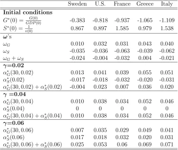
Table 2: Initial conditions (five countries, 2011), ω’s (Eq. (14)), annual inflowsα∗
G(te, γ)
(Eq. (22)) into G and α∗
S(γ) (Eq. (21)) into S for an escape at te = 30 and initial growth
rate γ = 0.02,0.04,0.06 (ι = 0.05, σ = 0.01). (Inconsistencies in the sums are due to
rounding errors). Source of initial conditions: http://data.worldbank.org/indicator.
These are values in the middle of each “iso-te” segment at which the line crosses the
α∗
G(γ, te) axis of Figure 4. This Figure shows that for all countries the escape is rapid with
bothγ = 0.02 andγ = 0.04. (For Sweden the point (α∗
G(30,0.04), α∗S(0.04)) in the middle
of the segment is just on the border between the rapid and delayed escape regions).
A high initial growth rate of γ = 0.06 requires for all five countries annual inflows of
fresh money into both compartments between 1.7% and 7.1% of initial GDP. The escape
is still rapid for all countries except France and Sweden whose escape is delayed with
minimum stocks G∗(t) reached at times t
𝑮∗ 𝜸, 𝟑𝟎
[image:19.595.106.453.127.348.2]𝑺∗ 𝜸
Figure 5: Straight-line loci of (α∗
G(γ,30), α∗S(γ)) annual flows for five countries escaping
in te = 30 years. Initial growth rates γ range from 0.02 (low point of segment) to 0.04
(middle point) and 0.06 (high point). The dotted lines are for each country the right angle borders of the rapid escape region in Figure 4 (conditions C3, C4).
We emphasize the purely illustrative nature of these projections which are probably
too optimistic. Indeed, in its recent “Long-Term Budget Outlook” the Congressional
Budget Office predicts a much more protracted increase in the U.S. debt (CBO, 2013).
In their best-case scenario the federal debt held by the public is 65 % of GDP in 2038,
a date close to the year 2041 at which the exercise above predicts a return into positive
territory.
Our model can easily produce realistic delayed escape scenarios in line with the CBO
projections. As an example we specify a time of escape of 70 years instead of 30, an
initial growth rate γ of 0.02 and the same σ and ι of 0.01 and 0.05. Figure 6 shows the
resulting delayed escape with the debt bottoming out in tm = 40 years (2051) at a value
G∗(t
m) =−1.05, i.e. 105% of initial (2011) GDP (which cannot be compared tocurrent
GDP, whether total of held by the public). The annual flow out of S isα∗
S(0.02) =−0.018
as in Table 2 with γ = 0.02. The annual flow α∗
to 0.026: a later time of escape requires a smaller annual infusion of funds into G, 0.018
of which can be drawn from S.
2000
2020
2040
2060
2080
2100
1.2
1
0.8
0.6
0.4
0.2
0
0.2
0
2
4
6
8
G*(t) S*(t)
Year
G
*(
t)
S
*(
t)
0
t
e
[image:20.595.93.510.152.392.2]t
m
Figure 6: A possible delayed escape for the U.S. government stock G∗(t), with S∗(t) on
right axis. Transfer rate σ = 0.01, interest rate ι= 0.05, initial growth rate γ = 0.02 and specified time of escape te= 70 years (2081).
6
Policy prescriptions and caveats
6.1
Prescriptions
We now bring together guidelines policy-makers can follow if they wish to use our model
to devise strategies toward fiscal consolidation. Our model may be very simple but its
initial conditions reflect the fact that the prospects for fiscal consolidation depend not
only on the debt to GDP ratio but also, not unreasonably, on the velocity of money, an
indicator of economic activity. Given these initial conditions policy-makers first need to
specify realistic interest and transfer rates satisfying 0 < σ < ι. They also decide on an
escape horizon te they think is realistic. The required annual flows α∗G(γ, te) and α∗S(γ)
If policy-makers want the government’s stock to start increasing right away (“rapid
escape”) this can happen only with a small γ and will lead to an outflow from S. One can
put this flow to good use by diverting it into G which then requires a smaller infusion of
fresh funds. We can think of this diversion of funds from S to G as an annual constant
“adjustment” tax which then decreases in real terms over time. This “adjustment” tax
must not be confused with the (main) taxation implicit in σ, i.e. income and corporate
taxes which are proportional to the size of the economy (measured by the stock in S).
Policy-makers may prefer an escape with a larger initial growth rate γ. The higher initial
growth will require non-negative infusions of funds into both compartments (stimulus)
and cause the debt to increase temporarily (“delayed escape”) while still recovering in
time for an escape at the same time horizon te. If the annual flows corresponding to the
prescribedσ, ι, te andγ are plausible the corresponding policy is implemented. Otherwise
the policy-maker re-assesses the parameter values until he obtains plausible flows - as we
did for the five countries considered above.
In short, the model provides answers to policy-makers on both sides of the ideological
divide who may have agreed on a desirable time horizon te for fiscal consolidation. The
hawks will find solutions that reverse immediately the trajectory of the government’s
stock but at a cost of lower growth and higher annual constant “adjustment” taxes which
will also mean less borrowing by the government. The doves will emphasize growth and
lower taxes - which is no doubt desirable but will come at the cost of a delayed recovery
and more government borrowing. There are complications however.
6.2
Caveats
The prescriptions described above illustrate the fact that within our model quite different
policies can lead to the same long-term results. However we recognize that our model
is still mechanistic and ignores intangible factors and complex feedback mechanisms
be-tween fiscal and monetary policies that may render some policies more realistic, desirable,
monetary parameters in the model can vary independently of one another (or of initial
conditions, as we will see below). Although beyond the scope of this paper such
mech-anisms can be fruitfully explored through a ”Russian dolls”-type modelling that would
take us deeper and deeper into the heart of an increasingly detailed model. We would
start by taking apart (or “deconstructing”) the neglected but important transfer rate σ.
The obvious first step is to model the flow σS(t) as receipts minus outlays. Under the
assumption of a constant velocity of money v, receipts are crudely obtained as a (possibly
time-varying) tax rateτ applied to the gross domestic productGDP(t) = vS(t). Outlays
are equally crudely modelled as proportional to society’s size measured by its stock S(t)
with coefficient of proportionality ǫ. The transfer rate then becomes σ =τ v−ǫ. Within
this framework the initial S∗(0) which is now the inverse of the (constant) velocity of
money v cannot change without causing a change in σ. More generally, a time-varying
constraint of the form σ = τ(t)v(t)−ǫ(t) can be used to capture fluctuations of GDP
or diverse feedbacks resulting for example from Laffer-curve or fiscal multipliers effects.
These effects and feedbacks should not doubt incorporate other components of the model
such as the interest rate and the annual flows.
7
Conclusion
The uses and abuses of mathematics in economics have attracted criticism, much of it
justified (Ruiz Estrada and Yap, 2013). Mindful of this criticism we do agree with
Krug-man (2000) however that simple economic models must not be neglected, particularly
those with modest but well defined ambitions. Indeed ours is a ”toy model” which
at-tempts to capture the essence of the mechanisms required to keep a government ”afloat”
- or to bring it back to solvency when it is in debt. We conceptualized the resulting
fiscal consolidation not as an equilibrium, the standard approach in economics, but as
an asymptotically exponential growth of money supplies. Endless exponential growth is
a mathematical construct however. Once the system has escaped the debt trap we trust
by spending more in Society - perhaps even making σ at least temporarily negative. The
government’s long-term aim then is to keep its budget at or near an equilibrium. This
“fi-nancial” equilibrium is not unlike the nutritional equilibrium experienced by populations
of the past once they had escaped the Malthusian trap (Komlos and Artzrouni, 1990).
A highly simplified model has shortcomings. One can dispute the central role played
in our model by society’s slightly nebulous ”money supply” S(t) (measured here by the
M2 money supply). Many important factors are omitted such as inflation, population
growth, consumption, savings, investments, to name just a few. Also a positive “fiscal
flow” σS(t) (i.e. a primary surplus) may not be a surprising escape condition. We still
need to know how realistic the model is and what combination of the “fiscal flow” σS(t)
and of the annual “monetary flows” αG and αS are needed in order to achieve an escape
at some reasonable prescribed time.
We have provided answers to these questions on two levels: first by showing that at
least for the U.S. there were parameter values for which the model’s trajectory
approxi-mated well the evolution over 32 years of the government’s and society’s stocks of money;
second, by showing that for five countries with debts to GDP ratios in the 38 % (Sweden)
to 111 % (Italy) range there are realistic parameter values which yield optimistic escapes
in 30 years. A realistic delayed escape is obtained for the U.S. in 70 years. Unrealistic
pa-rameter values are required for an escape in 10 or 20 years. We think this could well be the
case for any projection model, however complex or simple. In that sense the usefulness of
our (or any other) simple model lies in its ability to capture fairly accurately and robustly
the salient features of the system under study. For these reasons we believe that despite
its simplicity our model provides policy-makers with general, quantitative guidelines that
might help them find sensible solutions to the burning problem of preventing the train
wreck facing many economies caught in a debt trap.
Acknowledgement
References
Annicchiarico, B., Di Dio, F., Felici, F. 2013. Structural reforms and the potential effects
on the Italian economy. Journal of Policy Modeling, 35, 88-109.
Bernanke, B. 2010. Implications of the Financial Crisis for Economics, Conference Co-sponsored by the Center for Economic Policy Studies and the Bendheim Center for Finance, Princeton University, Princeton, New Jersey, 24 Septmber 2010.
Cecchetti, S., Mohanty, M.S. and Zampolli, F. (2010) The future of public debt. BIS
Working Papers No 300. Bank for International Settlements, Basel, Switzerland.
Congressional Budget Office. 2013. The 2013 Long-Term Budget Outlook. (September 2013), Pub. No 4713. http://www.cbo.gov/publication/44521.
Cottarelli, P. 2013. The austerity debate, in L. Paganetto (ed.) Public Debt, Global
Gov-ernance and Economic Dynamism, Springer Verlag, Italy, 301-308.
Hauptmeier, S., Sanchez-Fuentes, A.J. and Schuknecht, L. 2011. Towards expenditure rules and fiscal sanity in the euro area. Journal of Policy Modeling, 33, 597-617.
Herndon, T., Ash, M., and Pollin, R. 2013. Does High Public Debt Consistently Stifle
Economic Growth? A Critique of Reinhart and Rogoff.Working Paper No 322.Political
Economy Research Institute, University of Massachsetts, Amherts.
Knibbe, M. 2013. Looking at the right metrics in the right way: a tale
of two kinds of models, Real-world economics review, 63, 25, 73-97.
http://www.paecon.net/PAEReview/issue63/knibbe63.pdf
Kocherlakota, N. 2010. Modern Macroeconomic Models as Tools for Economic Policies
(2009 Annual Report).Banking and Policy Issues Magazines, The Federal Reserve Bank
of Minneapolis.
Komlos, J. Artzrouni M. 1990. Mathematical investigation of the escape from the
Malthu-sian trap, Mathematical Population Studies, 2(4), 269-287.
Krugman, P. 2000. How complicated does the model have to be? Oxford Review of Economic Policy, 16(4), 33-42.
Krugman, P. 2012. Blunder of Blunders. New York Times Blog, 22 March.
Marattin, L. Marzo, M., and Zagaglia, P. 2011. A welfare perspective on the
fiscal-monetary mix: The role of alternative fiscal instruments. Journal of Policy Modeling,
33, 920-952.
Merola, R., and Sutherland D. 2012. Fiscal Consolidation: Part 3. Long-Run Projections
and Fiscal Gap Calculations.OECD Economics Department Working Papers, No 934,
OECD Publishing.
Padoan, P.S., Sila, U., van den Noord, P. 2013. The sovereign debt crisis in Europe:
how to move from bad to good equilibrium. in L. Paganetto (ed.) Public Debt, Global
Ratto, M., Roeger, W. and in’t Veld, J. 2009. QUEST III: An estimated open economy
DSGE model of the Euro area with fiscal and monetary policy. Economic Modelling,
26(1), 222-233.
Reinhart, C.M. and Rogoff, K.S. 2010. Growth in a time of debt. American Economic
Review, 100, 573-578.
Ruiz Estrada, M.A. and Yap, S.F. 2013. The origins and evolution of policy modeling,
Journal of Policy Modeling, 35, 170-182.
Salvatore, D. 2010. Growth or stagnation after recession for the U.S. and other large
advanced economies.Journal of Policy Modeling, 32, 637-647.
Saunoris, J.W. and Payne, J.E. 2010. Tax more or spend less? Asymmetries in the UK
revenue-expenditure nexus. Journal of Policy Modeling, 32, 478-487.
Solow, R. 2010. Building a Science of Economics for the Real World. House Committee on Science and Technology. Subcommittee on Investigation and Oversight. July 20, 2010.
Trachanas E. and Katrakilidis C. 2013. Fiscal deficits under financial pressure and
insol-vency: Evidence for Italy, Greece and Spain,Journal of Policy Modeling, 35, 730-749.
Tramontana, F. 2010. Economics as a compartmental system: a simple macroeconomic