Relational cartographic data structures for geographical information systems

cosc

460

- Honours Project

Department of Computer Science

University of Canterbury

RELATIONAL CARTOGRAPHIC

DATA STRUCTURES FOR

GEOGRAPHIC INFORMATION SYSTEMS

R. T. Pascoe

Supervisor : Professor J. P. Penny

Section

3.

TABLE OF CONTENTS

Title

Page

Table of Figures

Introduction

Cartographic Data Structures

Geographic Data Attributes 2 - 1

Spatial Attributes 2 - 1

Non-Spatial Attributes 2 - 1

Spatial Data Models 2-2

Vector Data Models 2-2

Tessellation Data Models 2-5

The Relative Merits of the Vector Model and the

Tessellation Model 2-8

Current Research into Spatial Models 2-9

The Vaster Data Model 2-9

Examining Relational Cartographic Data Structures

BEAUTIFUL, and the Model Proposed by Shapifc?and Haralick 3 - 1

The 12 Strncture 3 - 1

The Ordering of Tuples in the 12 Structure Techniques for Ordering the Tuples Storage Requirements

Generating a Polxy Relation

Introducing a Spatial Reference Index to the 12 Structure The Quadtree Spatial Index

The Proposed Set of Relations Conclusions

3-3 3-3

3-4

Table of Contents

Section

4.

5.

c

Title

GEO-QUEL : A Relational Geographic Information System

The Relations Used by ROIS

The Structure of the Mapinfo Relation The Structure of the Maprelation Relation The Structure of the V duinfo Relation Functions Provided by ROIS

Description of the Functions Centre Display Make Outline Restore Save Projection Scale

Implementation of the Functions

Conclusions Drawn from Experimenting with GEO-QUEL

Final Conclusions

References

Appendices

Specification of ROIS

The Example Structure used for Generating the Polxy Relation

Specification of a System with a Separate Vector Data Structure

Page 2

Page

TABLE OF FIGURES

Figure

Title

Page

2.1 The hierarchical structure of vector data model 2-2

2.2 An example of a vector data model 2-3

2.3 Freeman - Hoffman chaincodes 2-4

2.4 The encloding of a polygon boundary 2-5

2.5 An example of a square tessellation model 2-6

2.6 Hexagonal mesh 2-7

2.7 An example of a point quadtree 2-8

2.8 An example of a vaster model 2- 10

3.1 The calculation of the storage required by the 12 structure 3-5

3.2 The calculation of the storage required by the structure with

sequence attributes 3-5

3.3 The calculation of the storage required by the structure with

vector attributes 3-6

3.4 A summary of the storage requirements 3-7

3.5 An example of a relational data structure 3-8

3.6 The sub-cell numbering scheme 3 - 11

INTRODUCTION

"Geographic information systems (GISs) are computer-assisted systems for the capture, storage, retrieval, analysis, and display of geographic data" [ Clarke 1986 ].

Geographic information systems are used in an ever growing range of applications, in government agencies such as the department of Lands and Survey and the Post Office, in local body organisations such as sewage, water, and power boards, and in the private sector.

Ideally, most, if not all, of the information that users require would be stored in a GIS that is accessible to all users. Each user would be responsible for the integrity of its own contribution of geographic information to the system while having access to information provided by other users. For example, electric power boards would be responsible for accurately recording the location of underground and overhead power cables and would have access to the information recorded by the Post Office concerning the location of .telephone lines and the location of sewage and water networks provided by the local council.

Such a global GIS would be a distributed system with the information for individual areas being stored locally. By localizing the information most frequently asked by users, to a particular county for example, the information can be retrieved without the transmission delay that is expected if a centralised GIS is being used. So, for example, the information for Christchurch would be stored in, or near, Christchurch rather than in a centralised GIS at Wellington. If at any time a user required information not kept locally it should be possible to retrieve it from the appropriate localized GIS through the connecting communication network. Powerful workstations like the Sun family are demonstrating that the hardware required for the envisaged distributed system is becoming increasingly accessible.

The ease with which the idealistic concept is described and visualised above belies the substantial research required to transform such a concept into a practicable system. In particular research into distributed relational database systems with the facility to split relations horizontally.

Introduction

Page 1 - 2

The purpose of this project is to investigate the suitability of the relational data model in preference to either the hierarchical data model or the network data model. The reason for considering the suitability of a relational database management system is the great flexibility in the way attributes and entities can be merged to produce new entities and structures. This flexibility might be utilized to access geographic information stored in a distributed environment.

Four applications of the relational data model [ Codd 1970] to geographic information are investigated: Beautiful by Warren Burton [ Burton 1979 ], a spatial data structure by Linda Shapiro and Robert Haralick [ Shapiro 1980], Geo-quel by Michael Stonebraker and Carol Williams

[Stonebraker 1975 ], and the 12 structure by van Roessel et al [ van Roessel 1986 ].

2.

Cartographic Data Structures

This section provides an introduction to one component of a geographic information system, the geographic data structure. Much of the material for this section is based on a more detailed discussion by Peuquet [ P euquet 1984 ] .

2.1

Geographic Data Attributes

The spatial attributes of a data entity describe the topography of the entity, usually in terms of coordinates in two, or three, dimensions. Other attributes of a data entity, referred to as non-spatial attributes, describe what the entity represents. A point, for example, may be described by the non-spatial data as an oil well that has a bore depth of 2 kilometres.

2 .1 .1 Spatial Attributes

Spatial attributes describe the topographical aspects of entities. These aspects are the shape of the entity as seen on a visual display screen or plotter, the location of the entity in the geographic data space, and its relationship with other entities:

1) What is to the left or right of an entity 2) How far away it is from other entities

3) What other data entities are contained within it

The essential problem is to design a data model that efficiently represents these two or three dimensional entities and the relationships between them.

2.1.2 Non-Spatial Attributes

Cartographic Data Structures

Page 2 - 2

2.2 Spatial Data Models

Vector and tessellation models are two basic types of spatial data models that have been evolved for

the spatial component of a GIS. The vector model is often described in terms of a hierarchical

structure since polygon boundaries can be described by a closed sequence of connected lines which

in turn are described by a connected sequence of points (figure 2.1).

The most well known type of tessellation model is the grid or raster representation. While this

model normally employs a square grid, it may also be based on any other pattern of a regular

polygon or polyhedron such as a triangle or a hexagon. The geographic data space is divided into a

regular mesh of either squares, triangles, or hexagons and data is stored for each cell of this mesh.

It is important to observe that in the vector model, data is stored for an e11tity (either a point, a line,

or a polygon) whereas in a tessellation model data is stored for each cell of the mesh. The

following two subsections examine these two models in more depth.

2.2.1

· Figure 2.1

The hierarchical structure of vector data models

Polygon

Arc4

~

Point 1 Point 2 Point 3 Point 4 Point 5 Point 6

Vector Data Models

The least structured of the vector data models is known as the 'spaghetti model'. Each entity in the

geographic data space is defined as a sequence of x, y coordinates; with no spatial relationships

being retained. Topological models evolved to record these spatial relationships by explicitly

recording adjacency information such as what polygons are either side of a line and the start and

Cartographic Data Structures

Page 2 - 3

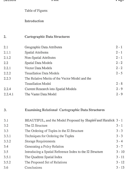
Figure 2.2

An example of a vector data model

Line 1

Line 6 2

3 7

Line 5

Line 3

CZ I

z

Polygon Line Points

1 1, 2, 3 1

2,3

2

2,6,5

3

3,4,5

2

3,5,6

5

5,9

6

3, 7, 8, 9

A particularly well known GIS built around the topological model is GBF/DIME (Geographic Base

File/Dual Independent Map Encoding) model used by the U S Census Bureau. An important

addition made by this system to the topological model was the explicit assignment of a direction to

each straight line segment by recording a from-node and a to-node with the coordinates (nodes are

the start and end points of a line segment). The resulting directed graph is used to automatically

check the integrity of the information stored by 'walking' around polygon boundaries. When it is

not possible to return to the starting point of the walk either a line segment is missing or a node

identifier is incorrect.

The main drawback to the GBF/DIME model, as with the previous two models, is that line

segments are not stored in any sequence, which means that, to retrieve the line segments that define

Cartographic Data Structures

Page 2 - 4

POLYVRT (Polygon converter), developed by Peucker and Chrisman [ Peucker 1975] resolved the problems of inefficient retrieval with these previous models by storing polygons, lines, and points separately in a hierarchical data structure. The advantages of doing so are two-fold. First the use of a hierarchical structure allows for entities to be constructed using other entities. For example, the boundary of a polygon may be a road. The road is an entity on its own but it is also used as a component of the polygon.

The second advantage of the hierarchical structure is that it reduces the information into levels of detail resulting in the selected retrieval of information specific to a query. If a request is made for a list of polygons adjacent to a given polygon, it is necessary only to retrieve information describing which polygons are to the left and to the right for the lines defining the boundary of the given polygon. The coordinate data is retrieved only when these polygons have to be plotted or displayed.

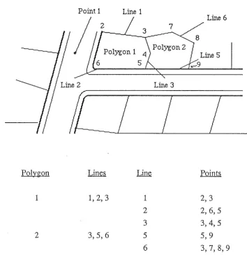
Chain encoding is a method for coordinate compaction and it is considered in this section because it is frequently an integral part of the vector and tessellation models discussed here. Freeman -Hoffman chaincodes [ Freeman 1974] consist of 8 directional codes between O and 7. The codes are assigned to the cardinal points of a compass plus the diagonals as shown in figure 2.3, and are used to encode line data super-imposed on a grid of given unit resolution. Figure 2.4 demonstrates this by encoding a polygon.

Figure 2.3

Freeman - Hofman chaincodes

3 2 1

4

5 6 7

Special coding sequences can be incorporated to identify special topological situations such as the intersection of lines and to further compact a sequence of repeated direction codes. Many variations of the chain coding scheme have been presented. The use of four, sixteen or thirty-two direction codes, rather than the eight, on a square has been suggested [ Freeman 1979] as well as the use of a hexagonal rather than a square lattice [ Scholten 1983 ] .

1:.:_·,

Cartographic Data Structures

Page 2 - 5

Figure 2.4

The encoding of a polygon boundary using Freeman-Hoffman chaincodes

One final variation is a scheme by Burton [ Burton 1979 ]. Unlike Freeman-Hoffman chaincodes,

where a directional code describes the next step of the vector from the position in which the previous directional code finished, the scheme suggested by Burton proposes that a directional code is not necessarily dependent on the previous code in the sequence.

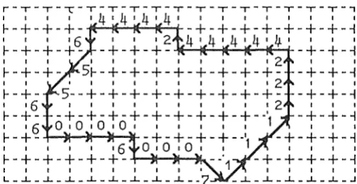
2.2 .2 Tessellation Data Models

Cartographic Data Structures

D

Cell

A B

A

Figure 2.5

An example of a square tessellation model

B

D

Density

50- 74 %

50 - 74 %

c

m

m

Cell

c

D

Page 2 - 6

lfil

Density

75 - 100 %

75 - 100 %

Triangular tessellations have the characteristic that the triangles in the mesh do not have the same

orientation. Because of this some operations such as the subdivision of these cells into smaller

cells (page 2-7) on this tessellation are harder to achieve than on either square or hexagonal

tessellations. However by incorporating a third coordinate, z, with each vertex of a triangle, this

characteristic can be used to an advantage when representing terrain and other types of surface data.

In particular the irregular triangular tessellation, where triangles in the mesh are not necessarily of

the same shape or size, can effectively represent the slope and direction of the geographic surf ace.

Hexagonal meshes have the geometric property of radial symmetry - all cells adjacent to a given cell

are equi-distant from its centre point (figure 2.6). This is useful for radial search and retrieval

Cartographic Data Structures

Figure 2.6

.All hexagonal cells adjacent to a given hexagonal cell are equi-distant from the given cells centre point.

Page 2 - 7

The cells of a tessellation model can be further subdivided and are referred to as nested tessellation models. Regular square and triangular cells can be further subdivided into smaller cells with the same shape. However, only the square cell can be subdivided into smaller cells with the same orientation. Hexagonal cells can be subdivided but not so as to completely cover the area of the original cell.

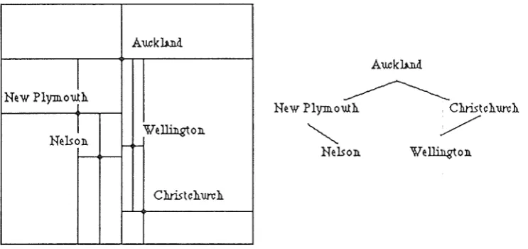
A very popular data structure for representing a nested tessellation model with square cells is the quadtree. Samet [ Samet 1984 ] has studied this structure in detail and outlined many applications for which this structure can be used. Of particular interest are the area quadtree and the point quadtree. Point quadtrees divide the geographic data space using data points. For example, the geographic data space could be divided by the location of cities. A city is chosen as the root and the geographic space is divided into four rectangular cells such that the city is the common vertex of the four rectangles. For each of these cells another city is chosen as the root and the cell is again subdivided (figure 2.7).

Cartographic Data Structures

Page 2 - 8

Figure 2.7

An example of a point quadtree

Auckh.n..d.

I

New Plymouth l

l

Nelson. ,

-Auckh.n..d.

~

New Plymouth Christchurch

~

/

Nelson. We~on.

Christch.urch

2.2.3 The Relative Merits of the Vector Model and the Tessellation Model

The critical difference between these two models is that points, lines and polygons are the components of a vector model, whereas areas of space, or cells, are the components of a tessellation model. The spatial relationships between the components of a vector model have to be explicitly stored, an example being the specification of which polygons are to the left and right of a line. These relationships must therefore be defined for a particular application. Tessellation models store these relationships implicitly, so that by investigating the properties of surrounding cells it is possible to determine, for example, whether the given cell is on the boundary of a particular polygon. This would be indicated by the surrounding cells having different properties than that of the given cell.

Theoretically both of these models are capable of representing any type of spatial data, but one model may be better suited to an application than another. Cadastral mapping is an application best suited for a vector model because of the type of data; lines and polygons. Tessellation models may be more suitable for vegetation/soil analysis because of the way in which the data is gathered, for example a survey area may be divided into a grid with measurements taken for each cell.

Cartographic Data Structures

Page 2 - 9

2.2.4 Current Research into Spatial Models

Research into spatial models appears to be heading in two directions [ Clarke 1986]. The first is to

provide very efficient conversion on demand between the existing vector and tessellation models

using special purpose hardware. The second is the design of a new super-flexible data structure

offering the advantages of both the vector and the tessellation models. One such model is called the

Vaster data model and was developed by Peuquet [ Peuquet 1983 ].

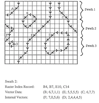
2 .2 .4 .1 The Vaster Data Mode[

The vaster model (figure 2.8) is a hybrid of the vector and tessellation models. The basic unit of

this model is the swath which consists of a raster component, or one scan line and a vector

component. A swath covers a constant, known range of y which, if encoded entirely in a raster

format, would be a group of scan lines. A scan line is a special case of the square tessellation

model where the cells are organised in a· contiguous row across the data space, usually in the x

direction.

The leading edge, the lowest y value of the swath, is a scan line and is used as an index record for

the swath. The index consists of a map-line identifier, x coordinate pair for each map line that

intersects the scan line. The encoding scheme is similar to that developed by MeITill [ Merrill

1973]. The remainder of the swath data is described in vector format. Each map line within the

swath is described using chain encoding at the same resolution as the scan line while any polygons

internal to the swath are listed separately.

The vaster model has two levels: at one level there are the scan lines, and at a lower level giving

greater detail is the vector chain encoding of the map lines. An advantage of this structure is the

ability to use only the scan lines as a quick means of browsing or sampling a very large database.

This could be applied usefully in a situation where the database may be remote from the user, as in

the case of a distributed system. At first only the scan lines would be sent as a generalised view of

the data space. Only when the user decides to look at a section of the data space in detail would the

chain encoded vector data be sent across the communication network. In a distributed system this

reduction in the quantity of data sent across the communication network would reduce the demand

Cartographic Data Structures

Page 2 - 10

Figure 2.8

An example of a vaster model

,

...

A

. JL

,,

JL

'

IJt

':,

l;(

~ '- ~

l;(

jt

IJt

p,:,

EJ.t

IJt

IJt

... If",

..

,.,

,

,,

Ji{

l;t

,,

Swath 2:

Raster Index Record: Vector Data:

Internal Vectors:

'If

,

'If

,

Swath 1

'.,

x

'.,

c\.t

L¥

IJt

~

,,

,, ,,

~

r>Jt

IJt

,.,

,,

l;(

'-

'-Swath3

~ b( , ,

B4, B7, ElO, C14

3.

Exaniining: Relational Cartographic Data Structures

Four relational geographic models were investigated: a model proposed by Shapiro and Haralick, [ Shapiro 1980 ], BEATUIFUL, proposed by Burton [ Burton 1979 ]. GEO-QUEL, proposed by Stonebraker and Williams [ Stonebraker 1975 ], and the 12 structure proposed by van Roessel et al [ vanRoessel 1986 ]. The first two models are are briefly discussed in section 3.1, the 12 structure is examined in 3.2, 3.3, and 3.4. GEO-QUEL is discussed in section 4.

3.1

BEAUTIFUL, and the Model Proposed

by

Shapiro and Haralick

BEAUTIFUL, the experimental geographic information system designed by Burton is based on research into the use of spatial or locational data types and specialised operations for attributes of these types in a relational database system. The three locational types proposed by Burton are called point, curve, and region. A similar approach of expanding the types of attributes in the relational model is considered. later in this -section, when the introduction of a vector attribute by the RIM relational database system is discussed in sections 3.3.1 and 3.3.2.

Shapiro and Haralick propose a set of spatial data structure types, which are based on the concept of an A/V (attribute/value) relation. From the set of spatial data structure types the required geographic information data structure is constructed. Due to the navigation (using pointer attributes) through the tuples in the relations that is necessary to create the sequence of lines in the boundary of a polygon, the approach taken by Shapiro and Haralick is not discussed further.

3 .2

The 12 Sructure

van Roessel et al gives three reasons for considering the relational approach for vector data structure conversion:

1) The simplicity and elegance offered by the relation as a structure for data representation.

2) To determine whether relational operators will permit the development of high level tools that can be used for the various data conversions required.

Examining Relational Cartographic Data Structures

Page 3 - 2

The 12 structure was designed as an intermediate structure for vector data conversion. However, in

this section the emphasis will be on using the (modified) 12 structure as a core to a relational

cartographic data structure. The definition of the 12 structure contains the following relations for

spatial data:

regpol: (regnum, polnum)

polarc: (polnum, arcnum)

archdr: (arcnum, strtnode, endnode, lftreg, rgtreg)

arcxy: (arcnum, x, y)

nodearc: (nodenum, arcnum)

The philosophy behind the design of this structure is to use "the hierarchy obtained by defining

more complex elem~nts in terms of their component parts - regions, polygons, arcs, nodes, and

vertex points - the most austere organisation is obtained by having each element reference its

subordinate elements. " [ van Roessel 1986 ]. Regions are defined in terms of polygons, polygons

are defined in terms of arcs, which are defined using nodes for start and end points, and a sequence

of vertex points (x, y coordinate pairs) connecting the two nodes.

An assumption is made by van Roessel et al that the tuples within a relation remain in a particular

order. It is required that "in regpol, the first polygon for each region is the outside polygon" where

the outside polygon defines the boundary of the region. This assumption on the organisation of

tuples within a relation makes the claim that the 12 structure is "strictly of first normal form"

inaccurate since one of the properties of relations specified by Codd [Codd 1970 ] is that there be

no dependency on the order of tuples in a relation. In section 3.3, a discussion is presented on

how to remove the assumption on the order of tuples in a relation from the 12 structure.

Non-spatial data describing regions, polygons, arcs, and nodes in the 12 structure is stored in a set

of relations consisting of one primary relation and other secondary relations:

The primary relation: attprime (elnum, attl, att2, att3, .. , .. , .. )

The secondary relation: attsec (attl, sattl, satt2, satt3, ... )

The link between the spatial elements (regions, polygons, arcs, and nodes) and their non-spatial

attributes is the common element identifier, elnum. Hence the domain of elnum would be the union

of the regnum, polnum, arcnum, and nodenum domains. Attributes in the primary relation can also

be used as keys for entries in the secondary relations to allow for more detail in the non-spatial

Examining Relational Cartographic Data Structures

Page 3 - 3

3

The Ordering of Tuples in the 12 Structure

The assumption made on the order of the tuples within a relation as part of the 12 structure is most undesirable and, as mentioned above, contravenes one of the properties that is expected of a relation. The use of ordering in the 12 structure is as follows:

1) The vertex point coordinates in the arcxy relation are stored in the sequence that defines the arc.

2) The arcs in the nodearc relation are stored in a clockwise rotation.

3) The arcs in the polarc relation are stored in clockwise order for normal polygons and counter-clockwise for island polygons.

4) The first polygon for each region in the regpol relation is the outside polygon.

The first three are similar: a group of tuples have to be kept in a predefined sequence. The fourth requires that one of a group of tuples be uniquely identifiable,which can be achieved by setting the value of the polnum attribute for the outside polygon of a region to be negative. Two techniques for explicitly specifying the required order or sequence of tuples are discussed; the introduction of a sequencing attribute, and the use of an attribute whose domain consists of matrices.

3 .3 .1 Techniques for Ordering the Tuples

Examining Relational Cartographic Data Structures

Page 3 - 4

An alternative to the sequencing attribute is provided by the RJM relational database system, which allows an attribute of a relation to have matrices as its domain. Such an attribute type is not permissible (on the grounds that attribute values must be atomic [ Date 1986] ) in the relational model. However, the departure from the standard relational model can be usefully applied to store the sequence of arcs for a polygon boundary, or the sequence of points for an arc. The vector attribute removes the need of having more than one tuple for a polygon boundary or a line since the respective components, lines or points, are stored in one vector attribute of a tuple. Thus the need for specifying a sequence for a group of tuples has been replaced by the implicit position of the components in the vector attribute.

The disadvantage with using the vector attribute is that in the RIM database system the join operation is not permitted on any attribute with a vector domain. Because such a facility is not available for this project the significance of this limitation is unknown. The advantage of allowing a vector attribute in a nominally relational c;latabase system is the more efficient utilization of storage space.

3.3.2 Storage Requirements

The introduction of the sequencing attributes to the polarc and arcxy relations increases the demand on storage space. To examine the effects on the required storage, mapping data files were surveyed to approximate the average number of points in a line, and the average number of lines in the

boundary of a polygon. The data files were stored in the colourmap data format [CSIRONET

1986] and the particular file studied the data was for Australian census boundaries. It was found that the number of points in an arc chiefly fell between 2 to 44 points, and that the number of arcs required to define a boundary ranged from 2 to 36, although the range was predominantly between 4 and 14. With this information, it is obvious that the point sequencing attribute or the arc sequencing attribute needs only to be a sixteen bit integer.

Examining Relational Cartographic Data Structures

Page 3 - 5

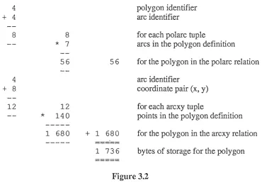
Figure 3.1

The calculation of the storage in bytes required by a polygon with 7 arcs, a total of 140 points using the 12 structure.

4

+ 4

8

4

+

12

8

*

56

12

*

1 680

56

+ 1 680

1 736

polygon identifier arc identifier

for each polarc tuple

arcs in the polygon definition

for the polygon in the polarc relation arc identifier

coordinate pair (x, y)

for each arcxy tuple

points in the polygon definition for the polygon in the arcxy relation bytes of storage for the polygon

Figure 3.2

The calculation of the storage in bytes required by a polygon with 7 arcs, a total of 140 points using the structure with sequence attributes.

4 polygon identifier

2 arc sequencing attribute

+

10 10 for each polarc tuple

*

70 70 for the polygon in the polarc relation

4 arc identifier

2 point sequencing attribute

+ 8 coordinate pair (x, y)

14 14 for each arcxy tuple

*

---1 960

+

--- =====

2 030 bytes of storage for the polygon

=====

Examining Relational Cartographic Data Structures

Page 3 - 6

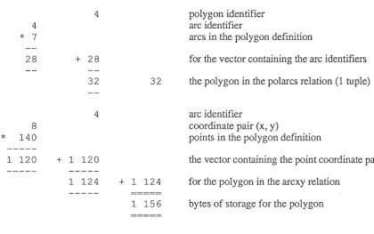
Consider another variation of the I2 structure with the relations:

polarcs (polnum. arcs)

arcpoints (arcnum , points)

The arcs attribute is a vector of arc identifiers, and the points attribute is a vector of point

coordin-ate pairs. The required storage space for the polygon with 7 arcs (140 points) would be 1 156

bytes (figure 3.3).

Figure 3.3

The calculation of the storage in bytes required by a polygon with 7 arcs, a total of

140 points using the structure with the vector attributes, as allowed by RIM.

4 polygon identifier

4 arc identifier

* 7 arcs in the polygon definition

28 + 28 for the vector containing the arc identifiers

32 32 the polygon in the polarcs relation (1 tuple)

4 arc identifier

8 coordinate pair (x, y)

* 140 points in the polygon definition

---1 ---120 + 1 120 the vector containing the point coordinate pairs

---

---1 ---124 + 1 124 for the polygon in the arcxy relation

- - - ₌₌₌₌₌

1 156 bytes of storage for the polygon

======

Figure 3.4 summarises the storage requirements of the I2 structure, and for the other two structures

with sequencing attributes and vector attributes. The data structure requiring the least storage is the

structure with vector attributes,using 66.59 percent of the space required by the I2 structure and

Examining Relational Cartographic Data Strnctures

Page 3 - 7

Figure 3.4

A summary of the storage requirements of the three data structures considered.

Data Structure

The 12 structure

The 12 structure with sequence number attributes The 12 structure with vector attributes

Storage Required

1 736 bytes 2 030 bytes 1 156 bytes

There are two reasons for the small space required by the structure using vector attributes. First there are no sequencing attributes required for the arcs and the points in the polarcs and arcpoints relations: the sequencing is implicitly stored within the vector attributes. The second reason is the non-repetitive storage of the polygon and arc identifiers in the polarcs and arcpoints relations. This is because there is one tuple in the polarcs relation for the arcs in the boundary of a polygon instead of one for each arc as in the other two structures discussed. Similarly there is only one tuple in the arcpoints relation for each arc rather than one tuple for each point of each arc.

In the above calculations the underlying structures employed by the database system are not considered. It is unclear how much influence these underlying structures would have on the storage space required and further experimentation would have to be performed to validate the above results.

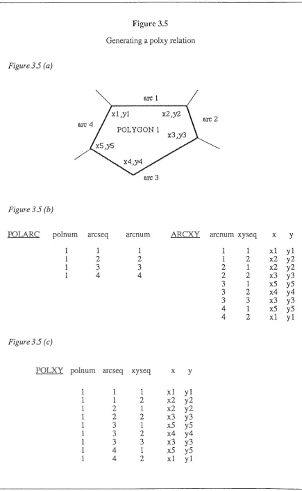
3

.4

Generating a Polxy Relation

Examining Relational Cartographic Data Stmctures

Page 3 - 8

Figure 3.5

Generating a polxy relation

Figure 35 (a)

arc 1

x2,Y2

arc 2

POLYGON 1

arc 3

Figure 3 .5 (b)

POLA RC

polnum

arc seq

arcnum

ARCXY

arcnum xyseq

x

y

1 1 1 1 1

xl yl

1

2

2

2

x2 y2

1 3

3

2

x2 y2

1

4

4

2

2

x3 y3

3

x5 y5

3

2

x4 y4

3

3

x3 y3

4

x5 y5

4

2

xl yl

Figure3.5 (c)

POLXY

polnum arc seq xyseq

x

y

1 1 1

xl yl

1 1

2

x2 y2

1

2

x2 y2

1

2

2

x3

y3

1 3 1

x5

y5

1

3

2

x4 y4

1

3

3

x3

y3

1

4

x5

y5

Examining Relational Cartographic Data Stmctures

Page 3 - 9

Figure 3 .5 ( d)

POLA

1 1 1 1 1 xl yl

1 2 2 1 2 x2 y2

1 3 -3 2 1 x2 y2

1 4 4 2 2 x3 y3

3 1 x5 y5

3 2 x4 y4

3 3 x3 y3

4 1 x5 y5

4 2 xl yl

Figure 3 .5 ( e)

POLXY

1 1 1 xl yl

1 1 2 x2 y2

1 2 1 x2 y2

1 2 2 x3 y3

1 3 -3 x3 y3

1 3 -2 x4 y4

1 3 -1 x5 y5

1 4 1 x5 y5

1 4 2 xl yl

The new polxy relation ( figure 3.5(c)) can be created by joining the polarc and the arcxy relations (figures 3.5(a), 3.5(b) ) on the common attribute arcnum. The sequence attributes (arcseq, and xyseq) in the two relations are also included in the new polxy relation to ensure that the sequence of points around the boundary of a polygon is not lost as a result of the join.

Another sequencing problem (referred to in section 3.3.1) arises when creating the polxy relation; if the sequence of arcs defining the boundary of a polygon is for a clockwise traversal of the boundary, yet some of the point sequences for the arcs correspond to an anti-clockwise traversal, the incorrect sequence of points will be created when the polarc and arcxy relations are joined to form the polxy relation. This is shown in figure 3.5(c) where the sequence of arcs are for a clockwise traversal, and the point sequence for arc 3 is for an anti-clockwise traversal.

Examining Relational Cartographic Data Strnctures

Page 3 - 10

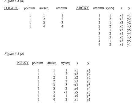
This sequencing problem occurs because one arc can be the boundary for two polygons, and the

one sequence of points defined for the arc will be in a clockwise direction for one polygon and in

the anti-clockwise direction for the other. It is necessary therefore to indicate the required direction

of the arc for a particular boundary.

The technique used by colourmap [CSJRONET 1986] is to set the arcnum attribute to be negative

when the desired sequence of points is the opposite to that stored for the arc. Employing this

strategy in the polarc relation (the new polarc relation is shown in figure 3.5(d)) the arcnum

attribute for arc 3 is set to be negative indicating that the required sequence of points for arc 3 is

opposite to that stored in the arcxy relation.

The creation of the polxy relation is now more complex, because it has to consider the sign of the

arcnum attribute to order the points correctly. If the value of the arcnum attribute in the polarc

relation is negative, then the sequence of points for the arc in the arcxy relation has to be reversed.

This is achieved by setting the arcxy sequence number attribute negative for the arc and listing them

in ascending order (for example, the sequence of arcnum values 1 2 3 negated and sorted in

ascending order is -3 -2 -1). Figure 3.5(e) is the final form of the polxy relation, which shows the

points in the sequence required for a clockwise traversal of the boundary of polygon 1. Appendix

B contains a detailed specification of the relations used in figure 3.5 for the INGRES relational

database system, and the QUEL macro for creating the polxy relation.

3

.S

Introducing a Spatial Reference Index to the 12 Structure

The purpose of a spatial index is to facilitate the efficient retrieval of features stored in a database

which covers a large geographic area. In particular, the use of a spatial index is to increase the

performance of a geographic information system for a query requesting information on features

within a specified region, or near a specific point in the geographic area. An example of such a

query is: list all the post office boxes within a 10 kilometer radius of the chief post office.

A description is given by Aronson and Morehouse [Aronson 1983 ], and by Dangermond

[Dangermond 1983] of the ARC/INFO GIS spatial indexing scheme, and a description of a spatial

indexing scheme using area quadtrees can be found in [ Palimaka 1986 ]. The scheme described by

Palimaka is the basic concept used by the relational geographic information system GEO-VISION.

The following two sub-sections, 3.5.1, and 3.5.2 describe the quadtree spatial index, and an

implementation of the index for the 12 structure.

I

Examining Relational Cartographic Data Structures

Page 3 - 11

3 .5 .1 The Quadtree Spatial Index

A cell is rectangular in shape and covers a part of the geographic area specified by the coordinates of either pair of diagonally opposing comer points. Arbitrarily the bottom left hand and the top right hand comer points of a cell have been chosen. The decomposition scheme outlined by Palimaka splits a cell into four equal sub-cells (figure 3.6) when the number of features (polygons, lines, and points) associated with the cell exceeds a specified number, called the split threshold. If

the number of features in any of these sub-cells exceeds the split threshold then they are further subdivided. Over a period of time features may be removed from the geographic data. If the number of features contained within four sub-cells sharing a common comer point falls below another specified number, called the merge threshold, then the four sub-cells are merged together to form a cell.

Figure 3.6

The sub-cell numbering scheme

2 4

1 3

Examining Relational Cartographic Data Structures

Figure

3.7

The quadtree addressing scheme for cell identifiers

1 2

B

A ~

A

3.5.2 The Proposed Set of Relations

2 3 4 1

A ~

2 3 4

A

(134)

The Cell-Feature Relation : Cellfeat (Cellid, Featid, Featype)

2 3

B

(430)

Page 3 - 12

4

The cell-feature relation specifies each feature that is either completely or partially defined to be within the specified geographic area of a cell. If point(s) of a feature are on the boundary of some cells, then the feature is associated with all of those cells. The cellid attribute is the cell identifier described above. The domain of the featid attribute is the union of the polnum, arcnum, and nodenum attribute domains. The featype attribute identifies the type of feature in a cell where the permissible features are; a polygon, a line segment, or a point.

The Cell-Location Relation : Cellocn (Cellid, Minx, Miny, Maxx, Maxy)

Examining Relational Cartographic Data Structures

Page 3 - 13

- 3 .6 Conclusions

Conclusions are now drawn about the three data structures,

1) The 12 structure, as defined by van Roessel et al.

2) The 12 structure, with sequencing attributes.

3) The 12 structure, with vectors allowed as attributes.

Only the second of these satisfies the requirements for relational data structure, as defined by Date

[Date 1986].

It has been shown that the third of these offers substantial storage economy. While the relational purists may dislike the departure from the fully relational structure, there seems no major difficulty in keeping the vectors of the third structure in a separate structure from the basic relations, with a link attribute connecting the data in the vectors and the relations. An experimental implementation along these lines was developed with the INGRES database system.

The elements of the vectors are stored in a linked list and the vectors are collected in two arrays, one for vectors containing the arcs of a polygon boundary, and the other for the vectors containing points of an arc. INGRES is used to implement the spatial indexing scheme described in section 3.4 with the featid attribute used as the key into the two arrays of vectors. This is not a practical implementation that can be used, but it demonstrates that it is possible to store the vectors in a separate data structure. A detailed specification of the implementation can be found in Appendix C.

4. GEO-QUEL · A Relational Geographic In

for11zation

Systeni

GEO-QUEL is a specialized retrieval and display utility built on top of Ingres [ Stonebraker 1976 ] a relational database management system. GEO-QUEL is intended to supplement the existing query language of INGRES, QUEL, with commands or functions specifically required for a geographic information system. The motivation behind GEO-QUEL is the idea that relations could be employed to store graphic data structures. In the article outlining the approach taken to implement GEO-QUEL a description of the relations used and the functions provided is given.

Because the relational database available for this project was Ingres, it was decided to implement a system, called ROIS (Relational Geographic Information System), based on the description of GEO-QUEL. The relations are those specified by Stonebraker; in practice one would want relations in third normal form. However the interest in this exercise is to assess the value of using the macro facility in QUEL to provide· fuctions to manipulate the relations. The following

'

sub-sections 4.1, and 4.2 describe the relations used by ROIS, and the functions provided to manipulate these relations.

4.1

The Relations Used

by

RGIS

There are three types of relations within ROIS: 1) Mapinfo:

For each map in the system there is at least one of these relations to describe ar least one aspect of each map. For example one mapinfo relation, called NZcoast, could contain data that describes the coastline of New Zealand, while another, called NZPolBound, could contain the data describing the political boundaries for New Zealand.

2) Maprelation:

For each mapinfo relation there is one tuple in this, the relation called Maprelation. Each tuple records the parameters for the most recently saved display by the user.

3) Vduinfo:

GEO-QUEL : A Relational Geographic Information System

Page 4 - 2

4.1.1 The Structure of the Mapinfo Relation

There is one mapinfo relation for each map in the system. This relation consists of at least nine attributes:

1) xl 4) y2 7) intensity

2) yl 5) plztype 8) groupid

3) x2 6) graphchar 9) zoneid

The first four attributes are the x and y map coordinates of the start and end points of a line segment. When the start and end points are equivalent the tuple represents a point rather than a line segment. The fifth attribute, plztype, specifies whether the tuple is a point, a line, or a zone. Attributes six and seven are used for graphical representation. In particular, if the tuple is a point then the value of the graphchar attribute is plotted on the screen. A group of line segments can be used to describe a line, an object, or a polygon. The eighth attribute is used to identify which, if any, group the tuple belongs to, while the ninth attribute records which zone the line segment or point belongs to. Other non spatial attributes can be included in this relation to further describe the tuple.

4.1.2 The Structure of the Maprelation Relation

This relation, called maprelation, is used to describe how each map in the geographic information system was last displayed. The relation consists of seven attributes:

1) mrelaname 4) ycentre 6) ymag

2) mrelowner 5) xmag 7) shadek

3) xcentre

GEO-QUEL : A Relational Geographic Information System

Page 4 - 3

The two attributes xcentre and ycentre record the x and y map coordinates specified to be the centre point for the most recently saved display of the map. Similarly, attributes xmag, and ymag, record the scale factor for the x and y axis of the most recently saved display of the map. The seventh attribute, called shadek, is used to record information on the distance between shading characters for the graphical presentation of the map.

4 .1.3 The Structure of the Vduinfo Relation

This relation is used to record inf01mation about the graphics terminal required by the display software. There are three attributes; one for the name of the terminal. and the other two for the maximum x and y screen values. It is assumed that the minimum x and y screen values are zero.

4.2

Functions Provided

by

RGIS

This section describes the functions provided by RGIS, and how they are implemented.

4 .2 .1 Description of the Functions

4.2.1.1 Centre

Syntax: centre at <x, y > \g

centre <relation name> on group <groupid> \g

There are two forms of this command: the first specifies the point of the map which is considered to be the centre of the screen for display purposes. The second requests the centre of the screen be calculated so that the specified group of the named map (relation name) is seen to be in the centre of the graphics screen. In both cases the dsptemp maprelation tuple is updated.

4.2.1.2 Display

Syntax: display \g

GEO-QUEL : A Relational Geographic Information System

Page 4 - 4

4.2.1.3 Make

Syntax: make <relation name> \g

This command is a combination of the outline and restore commands. The make command retrieves into the temporary display relation the named map with the display parameters saved in the appropriate maprelation tuple. This command corresponds to the view command described in the article on GEO-QUEL. The reason for the different name is to avoid clashing with the view command provided by the INGRES query language which creates a virtual relation.

4.2.1.4 Outline

Syntax: .outline <relation name> '.i_g

This command retrieves the map stored in the named relation, calculates the centre of this projection, and the necessary scaling factors. to allow the entire map to be viewed on the screen,

4.2.1.5 Restore

Syntax: restore \g

This command repaces the x and y scaling factors, and the centre point of the dsptemp relation with the values from the maprelation tuple appropriate for the map currently being dispayed. It is the complement command to the save projection command described below.

4.2.1.6 Save Projection

Syntax: save projection \g

This command replaces the x and y scale factors, and the centre point, in the maprelation tuple for the current map with the respective values currently stored for the dsptemp tuple. This results in the projection generated by the user in the temporary display relation (dsptemp) being stored for the appropriate maprelation tuple of the map.

4.2.1.7 Scale

Syntax: scale at <$xmag, $ymag> \g

GEO-QUEL : A Relational Geographic Information System

Page 4 - 5

- 4 .2 .2 Implementation of the Functions

All but one command, the display command, are implemented by defining macros in the Ingres query language QUEL. A listing of these macros can be found in appendix A, along with a small C program using equel (embedded QUEL) to retrieve and display graphically information from the database. A graphics emulator, called Griffin Terminal, provided for the Mackintosh is used to emulate a Tektronics 4012 graphics screen. An elementary line clipping algorithm [ Harris

1984 ] implemented by the author is employed to resolve the display of lines that are not

completely visible on the graphics screen.

4.3

Conclusions Drawn from Experimenting with GEO-QUEL

Using relations to store both spatial, and non spatial geographic data allows the data to be manipulated using the query language provided by the relational database. The use of the relational operators, and functions provided by the INGRES query language QUEL allows the design of powerful macros. These macros can achieve most of the processing that would normally be written in a programming language, like C, if the data were stored in a customized data structure. These macros are often easier to write because the data is dealt with at a higher level of abstraction, with relations instead of files and pointers.

The set of relations specified by GEO-QUEL is not very useful because of the lack of consideration given to the hierarchical nature of the spatial data. For example, the definition of a line on the boundary of two adjoining polygons is expressed twice, once in each group of lines for a polygon.

- 5.

Final Conclusions

The necessity to retain the sequence of points in an arc, and the sequence of arcs in a polygon boundary result in an inelegant relational data structure. The use of sequence numbers to retain this ordering, along with the repetitive storage of the polnum attribute for each arc in a polygon boundary, and the arcnum attribute for each point in an arc, increases the storage space required. The introduction by the RIM database system of an attribute whose domain is a set of matrices, or vectors, results in a much more elegant data structure. However, the introduction of this attribute is a departure from the relational data model which may upset the relational purist.

Research into the design of a distributed relational data model indicates that the relational model can be successfully employed in the distributed environment. The concept of horizontally splitting relations such that data in a relation can be stored at several different locations is a major sticking point and further research is being conducted ino the concept. It is this concept that is of particular interest because the division of the cartographic data such that the data for a particular county or city can be stored locally where it is most frequently accessed could be achieved by horizontal splitting of the relations. The localised data would be accessable to non-local users through the connecting network, provided they were authorised to do so.

Aronson 1983

Burton 1979

Burton 1979

Clarke 1986

Codd 1970

CSIRONET 1986

REFERENCES

P. Aronson, and S. Morehouse, "The ARC/INFO map library: a design for a digital geographic database", Proceedings AUTO-CART volume 6, number 2, pages 372-382.

W. Burton, "Implementation of the binary searchable grid chain representation for curves and regional boundaries", Geoprocessing, volume

1, number 2, pages 37-52

W. Burton, "Logical and physical data types in geographical information systems", Geoprocessing, volume 1, number 2, pages 167-181

K.C. Clarke, "Advances in Geographic Information Systems", Computing

Environment, Urban Systems Volume 10, number3/4,pages 175-184

E.F. Codd, "A relational model of data for large shared data banks",

Communications of the ACM, volume 13, number 6, page 377-387

"CSIRONET Reference Manual No 19, Command Driven Colourmap, User's Guide, Version 1" Graphics System Section, CSIRONET.

Dangermond 1983 "A modern GIS system for large spatial databases", ACSM-ASP Fall

Con-vention Technical Papers, pages 81-89

Freeman 197 4

Freeman 1979

Hagan 1981

H. Freeman, "Computer processing of Line Drawing Images", Computing

Surveys 6, pages 57-97

H. Freeman, "Analysis and manipulation of line-drawing data, Proceedings

of the NATO Advanced Study Institute on Map Data Processing, Maratea,

Italy.

References

Harris 1984

Kent 1983

Merril 1973

Palimaka 1986

Peucker 197 5

Peuquet 1978

Peuquetl983

Peuquet1984

Page 2

D. Ha.ITis, Computer Graphics and Applications, published by Chapman and

Hall Ltd, 1984 ..

W. Kent, "A simple guide to five normal forms in relational database

theory", Communications of the ACM, volume 26, number 2, Pages

120-125

R.D. Merril "Representation of regions and contours for efficient computer

sear- ch", Communications of the ACM, number 2, pages 69-82

J. Palimaka, 0. Halustchak, and W. Walker "Integration of a spatial and

relational database within a geographic information system", ACSM-ASPR

Annual convention, volume 3, page 131

T.K. Peucker, and N. Chrisman "Cartographic Data Structures", The

American Cartographer 2, pages 55-69

D. Peuquet, "Raster data handling in geographic information systems" In G.

Dutton (Ed.) First International Symposiuum on Topological Data Structures

For Geographic Information Systems, Harvard Laboratory for Computer

Graphics and Spatial Analysis, Cambridge, Massachusetts

D. Peuquet, "A hybrid structure for the storage and manipulation of very

large spatial data sets", Computer Vision, and Image Processing, volume

24, pages 14-27

D. Peuquet, "A conceptual Framework and Comparison of Spatial Data

Models", Cartographica, volume 21, number 4, pages 66-113

Private com. 1985 Private communications, EROS Data Center, 1985.

S::imf'.t 1984 H. Samet, "The Quadtree and related Hierarchical Data Strnctures", A.CM

References

Scholten 1983

Shapiro 1980

Stonebraker 1975

Stonebraker 1976

van Roessel 1986

Page 3

D.K. Scholten and S.G. Wilson, "Chain coding with a hexagonal lattice",

IEEE Transactions on Pattern Analysis and Machine Intelligence, volume 5,

pages 526-533

L.G. Shapiro, and R.M. Haralick "A spatial data structure", Geoprocessing,

volume 1, number 3, pages 313-337

M. Stonebraker, and C. Williams, "An approach to implementing a geodata

system", Proceedings of the workshop on databases for interactive design,

pages 67-77

M. Stonebraker, E. Wong, P. Kreps, and G. Held, "The design and

Implementation of INGRES", ACM Transactions on Database Systems,

volume 1, number 3, pages 189-222

J. van Roessel, D. Bankers, V. Connochioli, S. Doescher, G. Fosnight, M.

Wehde, D. Tyler, "Vector Data Structure Conversion at the EROS Data

Center" Final Report, Phase 1 (Draft)

Oct G 15:27 1986 dbase/RGISV3/appendixA Page 1

nE-?lat ion::

CJ \l-,l l·1 E! l' :

Tuplr:, ~'lic:lth::

f3,;1v(;~d unt .i. l. ::

1·~u,Y,b(;:-1r· of t1.lpl£c:f;:: Storage structure:

f~€,: la. t :i on t y pE! ~

><:l.

yl.

)(2

y·:::::

pl?:type 9 r•,=:\pl·1chE•. r·

i 1··, t en~" i t y

(;J l'<) up i c:I znne:i. cl

Pr~lc,\tioni

ClhWl8l" ::

TU p l (2 (\I i d t h ::

S,"\··.;ec:I until:

NuMber of tuples=

Storage structure= R eJ l '"' t i o 1·1 t y p £:·i =

!YI \'E,)]. n,':uY1(?

,y, r· <·::! 1 CJ ,,\Int? l' x ce1·1t e! 1"· yc<·,?nt er

)<i'irag y,y,,,~g

~.; h i::H:j •c;! !,;

R8.1.at:i.on=

[h,fflE! l' :

T 1 .. l p 1

f,·

S,7:\V"-'.·?d unt i. l ::

Number of tuples:

Storage structure=

f~0~1at:i.on type::

vc:I un,:1.1Y1E.~

IYl-::';.X ;.,:

typE2 f f f f c:~ ("' :i. i :i. type c ("' f ·(" f f :l

Tue Sep 2 23:54:28 1986

~::E,

pEtq(~cl hei:,\p , . .l!:5 e r l' r0 1 i::\'l; i o n

l €:?r1qt h l,E?ynci •

..'.1. li. l1. ti. 7 1

.

1Y1Bpreli::lt :i. Cltl

P<':\~:-Ctlf:'

r.'.1 :L

Tue Sep 2 23:57:46 1986

{j.

p,;i.qec:I hf;ir.:1.p

u ~SE? r r·e 1 ,,, t i. o t1

l.(;:1nqt 1-l

J. ~':i

{3 {1. {( (j. t.:1.

.-

.

Tue Sep 9 23=38=03 1986

:l

p21\:.Jf?ci h1:~ap

user r•el;:,tion

type length keyno.

("'

i

:LO

Oct 6 15n27 1986 dbase/RGISV3/appendixA Page 2

:i.

range of scrn is vduinfo range of mr is maprelation

range of ci is cisrtemp

l'an1.:.:J(3' of dt :I. :i.·::,, dte,Y,p1

range of dt2 js dtemp2

.range of dt3 is dtemp3

range uf dt4 is dtemp4

\q

{defjne; centre at $x,$y; \

replace mr(xcenter=$x, ycenter~$y) \

1,,J , ... , 1::?. r (;,~ 1Y1 i~ ,, 1Y1 r <;;i 1 n <':\ 1Y1 C'·? "''' 11 d ~, pt El ,Y, p 11 }

{define; centre Sr on group $g; \ df?.JE?tfc-'1 dti.1. \

d,:,:!JE1_tC:-? dt2 \

range of Mis $r \

ap pt?ncl t: () d t E?JYI p~? ( >< 1 :::::!'(1. >< :I. '/ y :l ""'1Y1" y :L. ){ ;;::::::,y, .. )( 2. y2:::::,y,. y;::) \

where m.groupid

=

c!t?.lc"!te c:lt1 \

cl. p p (~) '1 d t: n d t (!·) 1'(1 p :I. ( IYI i n )( "'" IYI :l n ( d t :::~. i( :I. ) ·, tYI i n y :,:: IYI i t1 ( cl t 2 • ':! :I. ) ., \

maxx

=

=

a p pend t a cl t

t,~

maxx

=

=

replace mr(xcenter

= \

( 1Y1 i n ( c:I t :I. • 1Y1 i n >< ) + ( ( 1Y1 B >< < d t :I. • ,v, ax >< ) ((I i )") ( d t; j, • tYI i )") >< ) ) I~;:: ) ) ., \

ycm·1t f:? r ::= \

( Ii'! :i. n ( d t :I. • IYI i n y ) + ( ( IYI c:l >< ( d t :I. • 1'(1 i::'I )( y ) -· tYJ i n ( cl t :I. • 1Y1 i n y ) ) / 2 ) ) ) \

'\.

J

v~hr:0?1'('0 1Y1)''., 1Y1l'~01n.,:\1Y1f:·? ::o: 11dE,p·tE?1Y1p11 \

{d<-.?fin1';.':; rf::1!:,:torf:? :; \

cl ''=! l f:? I; r.:·? d t ~:j \

}

append dtemp3(mrelname

=

v~hr.,-:i r'F! ,r, r'. 1Y1 rt::i l. n,,,\i'i1(,? == 11 d <;;pt E·)1Y1 p 11 \

c:l0,ilet0'! dtt.1 \

append ta dtemp4(xcenter = mr. xcenter, ycenter=mr.ycenter,

><mag= mr.xmag, ymag

=

where mr.mrelname

=

replace mr(xcenter=dt4.xcenter, ycenter=dt4.ycenter, \

><mag= dt4 .. xmag, ymag - dt4.ymag) \

\.•·J h (·:,· r ,::,, 1Y1 r· ,, 1Y1 \" <·,) 1 l"l <',:\ 1'11 Ei ::,: 11 d r;; pt F.:2 ,Y1 p 11 \

{define; make $r; \

r (;;, •,~, t o r !·,? \

dE1lc:c•te _{citi.1. \}

i:,ppr-2nd dtr,,a,pt.'.1 ( ><CE"mt; ("!! r =• 1'11 r. XCE·int <'? I'., yct0nt e r::::,,y, r. ycent er'., \

)( 1Y1i::\(J ::::: 1Y1 , ... " )( 1Y1aq '/ y1Y1,'.1(.:.J '"" 1Y1 )" • y,r,aq) \ 1,,1 l"1E! l'[·) ,n r. ,r, r <-'.,·! J. 1·"1i:\1Y1(,·:' :::, 1' cl !::l p t s: 1Y1 p 11 \

1"r:.0pli','.C('2 t'11r(1Y11"€'!:l.r.Jvinf:~r· ::::. 11t·r11., ><ct:-?nte:-~1' .... c:ltf.~. xcent(~r., \

ycenter

=

=

ymag

=

1-,1 ht':! I"•'::.·! 1Y1 r' .. l'i1 r·,::,.i l ni:~1Y1f!:) ,,:: 11 c:l s p t f::.' 1Y1 p 11 \

\

[:

I '.:: . .

Oct 6 15:27 1986 dbase/RGISV3/appendixA.Page 3

}

{ c:i (:c' "f :i. i""i\°'.c:'; e;; C,::\ J. f:, s:\ t </; >< .₁ iiy :; \

n:::1 pl <,:\Cf0 1Y1 r' ( :< ir, c:.~ 'J ::,:: iJ; :<, yrY1 ,£\ g ::.·: t,y) \

1tJ he rr,i i"i1 r' .. 1Y1 r'r::: l. n <':\ft1(7:• ::·:: 11

cl

t,

{define; outline $r; \

d1:2letf,? d \

}

d <'°" J. <-:.,ti'? d t :I. \ cl f.,:]. f2t (',' c:i "C ~::; \

range of m is $r \ 1Y1 <'':\ ( ,; ~::, it,. !"" \

app~nJ ta dspteMp (dspx1=m.x1,dspy1=m.y1,dspx2=m .. x2,dspy2=m.y2, \

c:l·;;:;pr;ir'or .. tp:i.d ::::: ,v, .. r;;i1'nup:i.d, d:::;pzntlt?!:i.d :::: 1Y1 .. znn~7:!:i.cl) \ e;\ppe11c:I to t:lti:·,:1Y1p:I. (i"!1:i.n>< :::: 1Y1in(cl .. df;p><l), 1Y1:i.ny "''' 1Y1:i.n(d.dt:;pyi).1 · \

maxx

=

=

a p pen c:I t C) c:I t F::: i"il p :I. ( 1Y1 i n ){ :.::: 1Y1 i n ( d • cl s p >< 2 ) , ((I :i. n y ;co: IYI :i. r"l ( d .. cl s p y 2 ) "/ \

maxx

=

r<,·:iplac::Ei 1Y1r(><1Y1r:~g ,,:.: (scrn .. 1Y1a>,;>< I (,v,a><: (dt:l..1Y1i::IX><) 1Y1in (cl·l;;:l..111:i.n>())), \

y 1Y1aq :c::: ( :,;c l"'t'l" IYliC\ )( y I ( 1Y1<'.l.>( ( d t 1 • IYt,:":\){ y) IYI :i. 1·1 ( cl t 1. n 1Y1 :i. ny) ) ) ·.· :«:::· (·,~ n t r::~ r' "'' \

(t"r1:ln (c.lt:l.,Y,:i.n>:) + ((1Y1<-'"~X (c:lti .. 1Y1a><><) ·-· tY,in (dt:l. .. 1Y1:i.n>-:))/2))

ycG:~nt *:·? r ,:: \

(i"t,jn ·(dt:l..,Y,iny) + <<,Y,ax (dt:l.,1Y1i:1><y> - ,Y,in (c:lt:l..,Y,iny))/;?))

\

hlh(,~ rr.:,i ,y, r. 1Y1 l'E) 1 n.,;:\1Y1f'.·) '"' 11 _{d s; pt E~1Y1 p} 11 \

{def:i.1··,1:;;1; :.-5iJ.VE; pi"'OJE!Ction; \

dr:?l(:':.'t(-2 cJt!.1 \

append "\.: o cit c;,,,Y, pt.:,. ( tY, rr:,, 1 nat"t, E·? "" ,n r. 1Y1r,::11 c> l"'n<·,~ r, \

xcenter

=

xMag = mr. xmag, ymag

=

~'1hE·?r(·? 1Y1l', 1Y1\'(i"!ltV:":\1Y1f.? .. ::: "d~:;ptE,·:1Y1p11 \

replace mr(Mcentel"'

=

xmag

=

=

1

.'J I 1r-a rt:~ 1Y1 r. i"il r (:,:~ J. n c:\i"t1Ei ,·:, r.l t /.~ .. 1"(1 r·r-2 J. r, a,Y1f::? \

}

:1-t:i.ncluc:l<::i 11

. . . l<Jriff:i.n/rJri-,1phic1";. h11

fl:d f~ fin(,;, y ,y,;,, >< ~-'; 00

·!kl<-:'! f :i. ne y,Y, :i. n O :li:r::kif .i. 11(·:~ ><1i"1<":'l. \( !.'.:.; 1. 1

Hc:l,:-,1_{f:i. nr::1 ><1Y1:i. n} O

:II:1-1: flo21"'; J.><:I., J.yl., l><'.:::'..1 ly2., ><£(C<':\lt:-::, ys-,cal.E,i;

## fl.oat xcentre, yc8ntre;

m,:,1 :i. n ()

{

dii:;,p].2\y ()

}

Oct 6 15=27 19BG dbase/RGISV3/appendixA Page 4

f]. (")i'\t )( 'J )/ .. '} {

i f (y _>

i f' (y (

:i.f ( >(

y1'(1f:\ >{) c I

y1Y1). l'1) _c I

iUirf.!.)() C: I

.... , .. - ·-E:i; (1.; :? ;

;i, f ( )( >< IYI :i n ) c:: I :::: 1 ;

}

{

rE,it urn < c) ;

ch,c1 r ch:;

int ><C :::: ::?~5~5 .,

fl.t>i::lt ><.I., ><2.,

ye :;:_o 1. ~50.,

y :I., y2 ~

tHI: :i l"lc;J rii?.~'l "-.. i !.1. :I. CJ" rq :i. r:~::;

'l-1:Jt ,,o·:n,gi::,~ o ( cl is ds:;pt€i,'1Y1p

p:l.cc,dE·,

ff# range of mis maprelat:ion

v~hi le (ch ... gi:,·~tchl;\r' () ! e:~ , q') { .

p2coc:112,;

it.it l"f?t r':i.,,,?vF~ ( >:!:,;cr.:lle '"'' r'f1. ><1Yrt':\(J1 yscale=1Y1. yrYr<':\~;11 ><CEint rE•""'rY1, xce1··1tE1r1

## ycentre = m.ycenterl

~HF 1,,1 h E·i \' f:'1 1Y1. 1Y1 l" Et l , .. i c"Wr (it "" 11 cl s; pt r-D 1i'1 p "

:l:!::J·I: {

p l'' :i. n t; f ( II \ )•) fl ) 1; cj·J::lt }

H# n~t \' :i. (0)Vf::) ( J. >< :I. ,-:::c:1. d S', p >< 1 'I l y :I. ::::cj,, c:1£, PY 1 , ]. ><2r:::cJ u d s p><2' l y2:::::rJ. d ~,; py2)

·!t:M: {

pr :int f ( fl 1 >< :I. ,,::: ~:. f ., l y :I. ''"' •y,", f, l ><::;;: :::: if. f, 1 y2 :::: "/., f \ n 11

, l x :I., 1 y 1 .,

l l-<2, J.y2)

){ :I. _·- ( l<C + ( _{l>< :I.} ><C~~nt ,~F~) ·lt )-{ !:5Ci::\ J. e.) _" 1

y:I ... (ye + ( _{J.y:I. ycE-?i··it} r·E:;) ·H· Y!?jC,'':\lFi)

.

}( ~;~ ... ~ (

~-< C' + ( 1 >< :::~ hON

><C8t1t l'f~)

'*

y2 -· (ye + ( _{ly2 yce·nt} )" (:;') -:':<· _{Y S'> C ,::\ J.} fa"! )

.

p:l.code ~ code(x:1., y:I.); p2code

=

if ((plcod2 & p2cnde) -- 0) {

wl·,:i.J.r,;, (p:lcocle !0 " 0 11 p2cndE·,: !s::: 0) { /·l<· clip 1:i.nf:.~ '*·/

:i. f (y :l ) y1Y1i::\){) {

>< :I. -.. >t l + ( ( x 2 ... >< :I. ) ·l<· ( y 1Y1 <:':\ >< .... y 1. ) I ( y 2 ··· y l ) )

y :I. ::: y1Y1€:\>< ~ }

YIY1f.:\X) {