Deterministic and Stochastic Annual Scheduling
A thesis
presented for the degree of
Doctor of Philosophy in Electrical Engineering
in the
University of Canterbury,
Christchurch, New Zealand
by
T. S. Halliburton B.E. (Hons)
List of Illustrations List of Tables
List of Principal Symbols Abstract
i
CONTENTS
PAGE
Acknowledgements ;'{vii
CHAPTER 1
CHAPTER 2
CHAPTER 3
INTRODUCTION
SURVEY OF SOME POWER SYSTEM SCHEDULING METHODS 2.1 Introduction
2.2 New Zealand System Models 2.3 Deterministic Models 2.4 Stochastic Models 2.5 A Decomposition Method 2.6 Conclusions
OUTLINE OF A GENERAL MODELLING AND SOLUTION TECHNIQUE FOR RESERVOIR SCHEDULING
3.1 Introduction 3.2 Demand
3.3 Generation and Storage
1
6
7 10 11 17
19 19
20
21
3.3.1 Introduction 21
3.3.2 Hydro Reservoirs 22
3.3.3 Run-of-River Hydro 26
3.3.4 Thermal Power Stations and Their Cost 27
3.3.5 Equipment OUtages 28
3.4 Transmission Loss by D.C. Loadflow Loss
Coeff-icients 28
3.5 The Principle of Solution by Hamiltonian 32 3.6 Formulation of an Optimisation Problem 34
3.6.1 State Constraints 34
3.6.2 Control Constraints 34
3.6.3 Summary of the Model So Far 39
CHAPTER 4
CHAPTER 5
3.6.5 Justi:fication of Spill Modelling 3.7 Solution of the Mathematical Model 3.8 Conclusions
THE DEVELOPMENT OF A CONJUGATE GRADIENTS ALGORITHM 4.1 Introduction
4.2 A Formula for Conjugate Gradients
PAGE 41 42 43 45 45 46
4.2.1 Definition and Justification 46
4.2.2 A General Formula 47
4.2.3 A Simplified Conjugate Gradients Formula 49 4.3 Fletcher and Reeves Conjugate Gradients
4.4 A Reliable Conjugate Gradients Algorithm 4.4.1 Introduction
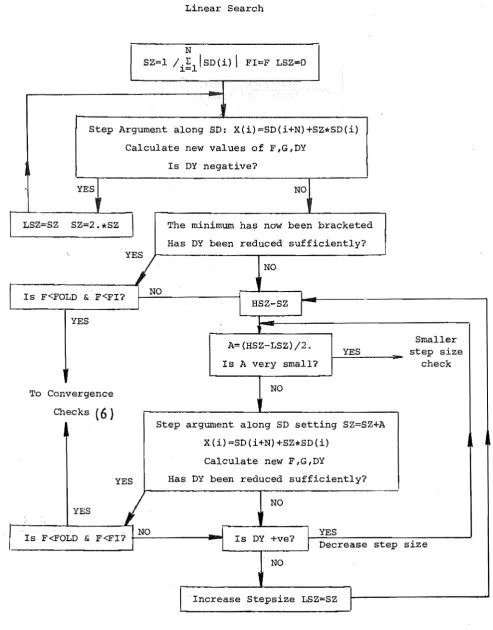
4.4.2 Linear Search Stepsize 4.4.3 Accuracy of Linear Searches 4.4.4 Controlling the Linear Search 4.4.5 Terminating the Search
4.5 Testing the Algorithms
4.5.1 The Rosenbrock Function
4.5.2 The Hydro-thermal Scheduling Problem 4.6 Conclusions
MODELLING THE NEW ZEALAND POWER SYSTEM 5.1 Introduction
5.2 Demand
5.3 Hydro Stations
,
5.3.1 Reservoir Modelling Principles 5.3.2 Run-of-River Stations
5.3.3 The Waikato System 5.3.4 Waikaremoana
5.3.5 The Waitaki System
5.3.6 Other South Island Reservoirs 5.4 Thermal Stations
5.5 Transmission Losses and the D.C. Link 5.6 Conclusions
CHAPTER 6
CHAPTER 7
CHAPTER 8
SOLUTIONS FOR THE NEW ZEALAND SYSTEM 6.1 Introduction
6.2 Summary of Problem and Solution Process 6.3 Optimisation Outputs for 1981 and 1982
6.3.1 Introduction
6.3.2 Comparison of Annual Statistics 6.3.3 Validity of the 1982 Simulation 6.3.4 Comments on 1982 Operating Strategy
PAGE 101 101 101 102 102 106 107 128 6.4 Effects of Some Modifications to the System 129 6.5 Comparison of Various Constraint Enforcement
Methods 131
6.5.1 Introduction
6.5.2 Control Constraint Methods 6.5.3 Penalty Function Tests
6.6
ConclusionsINTRODUCTION TO THE STOCHASTIC PROBLEM 7.1 Introduction
7.2 Some Possible Solution Methods
7.3 Inflow Modelling and Serial Correlations 7.4 A Linear Quadratic Gaussian Model
7.5 Data for Stochastic Models
7.6 Stochastic and Deterministic Solu~ions by Dynamic Programming
7.6.1 Methodology 7.6.2 Results
7.6.3 Discussion of Differences 7.7 A Linear Feedback Model
7.7.1 Development 7.7.2 Results 7.8 Conclusions
A POTENTIAL STOCHASTIC MULTI-RESERVOIR SOLUTION METHOD
8.1 Introduction
8.2 The Gaussian Plus Impulse Model
CHAPTER 9
8.2.1 The Concept - A Simple Form of Gaussian Sum
8.2.2 Model Development
8.2.3 Finite Differences Gradients 8.3 Results from the New Model
8.3.1 Preliminaries 8.3.2 Convergence 8.3.3 The Optimal 8.3.4 Simulation 8.3.5 Fuel Costs 8.4 Conclusions
CONCLUSIONS
9.1 Achievements 9.2 Implementation 9.3 Further Research
Strategy Check
APPENDIX I Listing of CGRADS Conjugate Gradients Computer Program
APPENDIX II Formulation of LQG Problem Equations
APPENDIX III Integration Details for Gaussian Plus Impulse Model
REFERENCES
PAGE
175 178 183 184 184 185 185 191 191 191
195 195 196 197
199
207
211
FIGURE 2.1 2.2 3.1 3.2 3.3 3.4 3.5 3.6 3.7 4.1 4.2 4.3
, 4.4
4.5 4.6 4.7 4.8 4.9 4.10
LIST OF ILLUSTRATIONS
Structure of the decomposition method
Two time step linear subproblem showing degeneracy problem difficulty
Load duration curve and three segment approximation
Conversion efficiency, water to electricity, at Benmore
Conversion efficiency, water to electricity, at Waitaki
Multi-stage decision process
Solution procedure by Hamiltonian of the hydro-thermal scheduling problem
Assymptotic transformation for controls
Piecewise parabolic transformation for controls
Calculation flow chart for conjugate gradients
(a)-(c) Fletcher and Reeves conjugate gradients algorithm flow chart
"Glitch" in contours of the hydro-thermal scheduling problem.
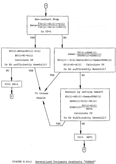
(a)-(f) Flow chart for generalised conjugate gradients algorithm, CGRADS
2-Dimensional Rosenbrock' function
Decrease in function value of 2-D Rosenbrock function with steepest descent
Decrease in function value of 2-D Rosenbrock function with FMCG, x 1 scaling of initial stepsize
Decrease in function value of 2-D Rosenbrock function with FMCG, x .001 scaling of initial stepsize
Decrease in function value of 2-D Rosenbrock function with CGRADS
"Scaled" 8 reservoir hydro-thermal problem. Decrease in function value when solved by steepest descent
FIGURE 4.11 4.12 4.13 5.1 5.2 5.3 5.4
"Unsealed" 8 reservoir hydro-thermal problem. Decrease in function value when solved by steepest descent
"Scaled" 8 reservoir hydro-thermal problem. Decrease in function value when solved by CGRADS
"Unsealed" 8 reservoir hydro-thermal problem. Decrease in function value when solved by CGRADS
Map of New Zealand showing locations of hydro reservoirs and thermal stations
The Waikato System
The Waitaki System
Model for Waitaki System
6.1 .(a)-(k) Results for the year ended 31st March 1982 simUlation
7.1 Demand pattern for one reservoir models
7.2 Inflows, total monthly averages for one reservoir models
7.3 Flow chart of stochastic dynamic program operations for
one time step
7.4 S.D.P. results - incremental fuel cost variation with
water storage
7.5
7.6
7.7
Mean inflows storage trajectories for S.D.P. showing convergence to a steady state trajectory.
Mean inflows storage trajectories for stochastic and deterministic D.~ s
Mean ± 0/3 inflows storage trajectories for stochastic and deterministic D.P~: s
7.8 Releases for t=l, stochastic and deterministic D. P. 's
PAGE 77 78 79 83 91 94 95 117 150 150 153 156 157 158 159
and linear feedback model with Gaussian distributed storages 160
7.9
7.10
7.11
Releases for t=5, t=12, stochastic and deterministic D.P,s and linear feedback model with Gaussian distributed storages
Mean inflows storage trajectories for S.D.P. and linear feedback model with Gaussian distributed storages
Mean ± 0/3 inflows storage trajectories for S.D.P. and linear feedback model with Gaussian distributed storages
161
170
FIGURE
8.1 8.2
8.3
8.4
8.5
Accumulation of uncertainty in storage
Storage probability density function evolution from t to t+l, with Gaussian plus impulse approximation
Releases for t=l for S.D.P. and Gaussian plus impulse model
Releases when optimisation begins at t=5, for S.D.P. and Gaussian plus impulse
Mean ± 0/3 inflows storage trajectories for S.D.P. and Gaussian plus impulse
PAGE
177
179
187
188
TABLE 3.1 4.1 4.2 4.3 4.4
LIST OF TABLES
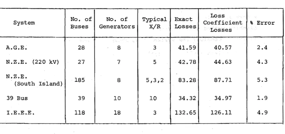
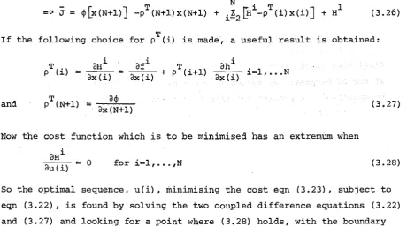
Tests of Loss Coefficients
Results for deterministic 8 reservoir hydro-thermal problem for various XLS and RSC
8 Reservoir problem solved by CGRADS. Number of iterations of each type and function value reductions
Order of occurrence of various iteration types for scaled problem solved by CGRADS
8 Reservoir problem solved by steepest descent. Average function value reductions
4.5 Gaussian plus impulse model solved by CGRADS.
5.1 5.2 5.3 5.4 5.5 5.6 5.7 5.8 6.1 6.2 6.3 6.4 6.5 6.6 6.7
Number of iterations of each type and function value reductions
List of reservoirs and thermal stations appearing the model
North Island hydro stations - physical data
South Island hydro stations - physical data
North Island hydro stations - performance
south Island hydro stations - performance
Thermal stations data
Storage limits on Lake Taupo
Tekapo storage limits
Comparison of optimisation output and NZE Annual Report, year ended 31 March 1982
Comparison of optimisation output and NZE Annual Report, year ended 31March 1981
in
Initial storages and final time targets for optimis-ations, and NZE Annual Report data
Cost of thermal fuel for various control convergence tolerances, 1982 year simulation
1982 year simulation - output of optimisation
Transmission losses as percentage of generation
Effects of various inflow levels. Table of annual load factors for thermal power stations
TABLE 6.8 6.9 7.1 7.2 7.3 7.4 7.5 7.6 7.7 7.8 8.1
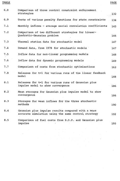
Comparison of three control constraint enforcement strategies
Tests of various penalty functions for state constraints
Monthly inflows - average serial correlation coefficients
Comparison of two different strategies for Linear-Quadratic-Gaussian problem
Thermal station data for stochastic model
Demand data, from 1978 for stochastic models
Inflow data for non-linear programming models
Inflow data for dynamic programming models
Comparison of costs from stochastic optimisations
Rf:leases for t=l for various runs of the linear feedback model
Releases for t=l for various runs of Gaussian plus impulse model to show convergence
8.2 Mean storages for Gaussian plus impulse model to show
convergence.
8.3
8.4
8.5
Storages for mean inflows for the three stochastic methods
[image:11.563.65.528.66.763.2]d. ~1
D
DY
ECC
ECO
erf(.)
G v G G
I
v
i
i
j
k
K
v
L(t,j)
L(X,A)
LIST OF SYMBOLS
- search direction vector.
- electrical energy demand (MWh).
- directional derivative.
- loss coefficient, matrix, for D.C. loadflow method.
- loss coefficient, vector.
- loss coefficient, scalar.
- error function.
- gradient~
- duration of load class j (hours).
- vector of generator energy outputs.
- generation from a river system (MWh).
- minimum generation (MWh).
- maximum generation (MWh).
- Hamiltonian.
- inflow (MWh).
inflow, one reservoir model, (GWh).
- mean inflow (GWh).
- load class index.
- conjugate direction index. - gain, linear feedback model.
- conversion factor for water, from equivalent energy value in reservoir q to value in reservoir q+l.
- water flow to energy conversion factor (MWh/cumec).
- number of load classes.
- index for inflow probability distribution points.
- transmission loss.
m - number of reservoirs.
MX v - range of releases possible from reservoir (MWh).
n p R v RR R
-v
-
R vs
v SD(i) SZ t T v u u v W v W(f)V WU v x xx
vx
-v-- number of reservoirs plus number of thermal stations.
- number of run-of-river stations - probability.
- reservoir water release (MWh).
- run-of-river stations index.
- minimum release (MWh).
- maximum release (MWh).
- spill (MWh).
- restart parameter.
- element of search direction vector.
~linear search step size. - time interval index.
- final time.
- tributary inflow (MWh).
-'release, one reservoir model, (GWh).
release at mean storage, one reservoir model, (GWh).
- unconstrained release.
- reservoir or thermal station index.
- penalty function weight, on state variables.
- penalty function weight on final time target state.
- penalty function weight on control variable.
- reservoir storage, one reservoir models, (GWh).
- mean storage, one reservoir models (GWh).
- reservoir storage (MWh).
- minimum storage (MWh).
X - maximum storage (MWh).
v
A
v
cr
cr
x
cr,
~
- probability of maximum storage.
- delta function (impulse).
- Lagrange multiplier.
- incremental cost of thermal fuel.
- mean of Gaussian.
- costate.
- unit step function - standard deviation.
- standard deviation of storage.
ABSTRACT
The optimisation of hydro-thermal power systems over a one year horizon
is investigated. The objective is to minimise fuel costs by appropriate
scheduling of releases from large hydro storage lakes. Fuel cost is the
principle avoidable expense in operating such a system as hydro station costs
are independent of power generated.
A deterministic model is described. It represents all stations fed
by each reservoir as one equivalent station. All generation and storage constraints
are handled. Transmission losses are determined by a simple d.c. load flow loss
coefficients method.
A Hamiltonian approach is used to convert this model to a static problem
which we can solve by a non-linear programming method. A conjugate gradients
algorithm was developed, with emphasis on robustness and accuracy, which successfully
solved a number of variants of the problem. As an example, the New Zealand system
is solved. It includes eight reservoirs, six thermal stations, and the transmission
constraint on a D.C. link.
A one reservoir equivalent of this system is used to study various
stochastic inflow effects. Stochastic dynamic programming is shown to give
quite different results to deterministic methods. A linear feedback algorithm
representing storage probability distributions by a Gaussian plus an impulse is
tested. This sub-optimal method does not suffer from the dimensionality
barrier of D.P. methods. It is thought to have the potential to provide a
ACKNOWLEDGEMENTS
I wish to thank my supervisor, Dr. H. R. Sirisena, for his guidance
over the five years of research for this thesis. His great patience, and
ability to generate enthusiasm when my research has seemed fruitless have
been consistent throughout this time.
Dr. J. Lermit of New Zealand Electricity made a very valuable
contribution in the early stages of my work with data for lake inflows etc.
Mr. M. Turner, also of N.Z.E., has assisted considerably with further system
data.
All the computer results in this thesis were obtained on the University
of Canterbury, Electrical Engineering Department's VAX 11/780 computer.
Without this machine, this thesis would not have been possible in its present
form. I am extremely grateful to Bill Kennedy for his tremendous efforts
with this computer, both in its initial installation and in ensuring that it
ran smoothly.
I am indebted to the University Grants Committee and New Zealand
Electricity for financial support during my studies.
Finally, I wish to thank Gordon Tillier of the N.Z.E., Christchurch,
draughting office and my typist, Beryl Nottingham, for their efforts in the
CHAPTER 1
INTRODUCTION
This thesis presents some efforts to solve the problem of optimal
annual sc?eduling of hydro-thermal power system operations. The objective
of such an optimisation is to minimise the cost of fuel burnt in thermal
power stations, by determining appropriate weekly water releases from large
long-term hydro electric storage reservoirs. The cost per MWh generated
at thermal stations varies greatly from those stations designed for supply
of short peak loads only, down to those intended for base load generation.
Hence the algorithm must try to ensure that the more costly thermal stations
are used as little as possible, that reservoir water is not wasted
unnec-essarily by spilling, and take· into account transmission line losses,
and the various physical system constraints.
A variety of optimisation problems, with differing time scales, can
be formulated for power system operat~ons. With a time scale of many years, is the optimal system expansion problem. A one week time horizon problem
might be solved to find detailed generation schedules, within the constraints
of desired total weekly generations determined by the annual problem. An
economic dispatch program could be re-run every 20 minutes or so to
deter-mine optimal machine loadings, minimise line losses, and check on system
security (e.g. line limits, equipment ratings).
whereas all the others are dynamic.
This is a static problem,
The annual scheduling problem was chosen for this thesis as it is
an especially interesting optimisation problem, not due to a desire to solve
this particular problem for its own sake. It involves reservoir inflows
which are variable, with considerable uncertainty over the one year time
scale. This gives opportunities to investigate stochastic control systems.
The problem is of high dimension - many reservoirs to schedule over each
time interval, and with many time intervals. (A 312 dimensional problem is
solved in Chapters 5 and 6). The power system data required is readily
available. By optimising a large, real system it was hoped that the
development of yet another optimisation algorithm of limited usefulness
would be avoided. A good example of what we wished to avoid is briefly
The structure of the problem is also interesting in that it consists
of a number of subsystems with only limited coupling. Each river system
with a chain of hydro stations along it, or in some cases only one station,
forms a subsystem. Coupling is largely restricted to the requirement that
total generation equals demand.
Research efforts began on a deterministic model, with a reliable
solution method. A model of the New Zealand system was solved with 8
large reservoirs (two of which are in series) and 6 thermal stations.
Then attention moved to stochastic models. Techniques are less well
developed in this area. So a simple model was used with attention
concen-trating on the aspects of the hydro-thermal problem which can not be
handled satisfactorily by established procedures.
The thesis proceeds as
follows:-Chapter 2 first describes previous work on the annual scheduling of
the New Zealand power system. None of .these methods appear to have been
used to schedule reservoir releases, in practice. Some representative
examples of deterministic and stochastic models are discussed to help
identify the state of the art, and to give a basis for the evaluation of
our work. A decomposition scheme which we experimented with,
unsuccess-fully, is described.
terms.
Chapter 3 gives the deterministic modelling technique in general
The problem is formulated as a large non-linear program to be ,
solved by the unconstrained, static hill-climbing algorithm of Chapter 4.
The various constraint enforcement. strategies and conversion from a dynamic
to a static problem are described.
Chapter 4 describes the development of a generalised conjugate
gradients algorithm, "CGRADS". A Fletcher and Reeves version was used
first. Problems encountered and the steps taken leading to the final
form of "CGRADS" are described. This was necessary to obtain reliable
solutions to our very difficult problem.
Chapter 5 applies the modelling technique of Chapter 3 to the New
Zealand system, and gives detailed model data. We consider this model
In Chapter 6, solutions to the New Zealand model are presented
in detail for one case. The validity of the results is discussed.
The various constraint enforcement methods experimented with are compared.
In Chapter 7 we first go through various aspects of reservoir inflow
modelling, to help understand the nature of the stochastic beast. Then
stochastic and deterministic dynamic program results are given for a one
reservoir model, followed by a linear feedback method. This method is
sub-optimal, but feasible for a multi-reservoir problem, unlike the dynamic
programming methods.
Chapter 8 develops the linear feedback method further by using a
non-gaussian distribution for water storages. This method, if developed
further could offer a practicable solution to the multi-reservoir stochastic
problem.
Chapter 9 concludes this thesis with comments on implementation of
a scheduling method. Some .ideas are given on how the work described here
could be extended to produce a computationally feasible, stochastic method
which could possibly be a useful, practicable solution to this problem.
All computer results given in this thesis were obtained on a VAX
11/780 computer.
The following papers were published in the course of research for
this thesis:
Sirisena, H. R. and Halliburton, T. S., "Long-term optimisation of
hydro-thermal power systems by gen~ralised conjugate gradient methods",
Optimal Control Applications and Methods, 2, pp35l-364, 1981.
Halliburton, T. S.and Sirisena, H. R., "Long-term optimal operation
of a power system", I.E.E. Froc., 129ptC, pp185-19l, 1982.
Halliburton, T. S. and Sirisena, H. R., "Development of a stochastic
optimisation for multi-reservoir scheduling", IEEE Trans Automatic Control,
CHAPTER 2
SURVEY OF SOME POWER SYSTEM SCHEDULING METHODS
2.1 INTRODUCTION
This chapter surveys a few examples of reservoir scheduling
algor-ithms to help put the ideas developed in this thesis into perspective.
A detailed study of any other method is not made as our method was not
inspired by, or developed from any other.
Extensive bibliographies on the topic exist. Rosenthal (1980)
gives a (by no means exhaustive) list of 100 papers and classifies them
according to their ability to handle:
( i) (ii)
(iii) (iv)
Multiple reservoirs
Multiple time periods
Stochastic inflows
Non-separable cost functions (F) as a measure of system
a
2Fbenefits Le.
o
for i .,. j.None of the 100 methods listed has all these desirable properties.
Sachdeva (1982) gives a bibliography for reservoir scheduling
methods with a variety of time scales. 110 of these refer to the long
term problems despite covering only the period 1960 to 1978. El-Hawary
and Christensen (1979) describe their own work on shorter time scale
problems in detail and are a source of references to literature on power
system optimisation generally.
Models developed for the New Zealand system are covered in more
detail than others, and are described separately in the next section.
Following this, some deterministic and then stochastic models are
described. Finally a decomposition method is given in some detail.
Considerable effort was expended.on,its investigation, as it:appeared to
2.2 NEW ZEALAND SYSTEM MODELS
No long term scheduling algorithm of the type described in this
thesis is in use by New Zealand Electricity, but a number of aspects of
the system have been modelled for optimisation purposes.
One of the first (McCooi
et aZ
(1966» was a simulation (not anoptimisation) to study the effect of diverting Tongariro catchment water
into Lake Taupo. Three reservoirs were modelled, all South Island storage
being lumped into one. Simulations were over one year's operation with a
one day time step. Fears had been expressed about the possibility of
flooding due to the extra lake inflows. As a result of the simulation,
lower lake levels were recommended, thereby reducing the possibility of
lake side flooding, despite higher mean flows.
Green (197la, b) used two dimensional dynamic programming to obtain
a giveneleotrical output from the three lower Waitaki stations as
econom-ically as possible. This involves minimising spill, operating with the
highest possible heads, and running generators at their peak efficiencies
as much as possible. A one day horizon and one hour time step were used.
McKerchar (1971, 1975) used deterministic dynamic programming and
synthetic streamflows to solve a system consisting of Lakes Pukaki and
Tekapo, and assumed quadratic thermal generation costs. He simulated
40 years of streamflows, then used linear regression to obtain reservoir
release as a function of the storage at the beginning of a time interval.
A one month time step was used.
Lusk (1972) describes the "Basic Rule Curve" method which has been
used by New Zealand Electricity (NZE). This involves producing a diagram
of storages against time. It indicates the storage level at which maximum
thermal generation has to be brought into use if an energy deficiency is
to be averted under the worst possible inflow conditions. This is a
security, not an optimisation device, however. It is used to draw up
guidelines which do take some account of economic operation. Lusk(l976) propose:
..
a trajectory method, based on that of Electricite de France (EDF)
(Daellenbach and Read (1976) ) • Trial and error is used to locate reservoir
storage trajectories which give incremental costs of thermal energy as near
Boshier and Lermit (1977) produced a network flow algorithm
intended primarily for estimating marginal energy costs. It involved
weekly time steps, seven reservoirs and the D.C. link constraints.
Each time interval was split into five load classes derived from the
load duration curve, as for the method described in Chapter 3. A l~
year time horizon was used.
Daellenbach (1979) proposed a stochastic dynamic programming method
decomposing the system into separate North and South Island subsystems,
joined by the D.C. link. A pricing mechanism would co-ordinate the
subsystems.
Reed (1979) adapts the E.D.F. trajectory method to give a
decompos-ition approach. He describes a detailed model involving losses and
trans-mission constraints. It is suitable for short term scheduling of a chain
pf stations, such as on the Waikato, and for the long term problem. An
example problem is solved. The.rnodel used includes six reservoirs and has
a'one week time step. 'The D.C. link is the only transmission constraint handled.
The possibility of a stochastic solution using the work of Rockafellar
and Wets (1976) on optimal recourse is considered. The same decomposition
method is used as in the deterministic case, but with a different hydro
subproblem.
N.Z.E. have developed a one reservoir stochastic method, but do not
appear to have published a description. It is based on the work of Stage
and Larson (196l), which is effectively a stochastic dynamic programming
method. It has been used to help estimate thermal fuel requirements.
2.3 DETERMINISTIC MODELS
Models which do not include the stochastic nature of inflows are
considered here. The first group of five models were not tested on
real-istic systems - only on simple contrived systems. The second group of
four were developed to produce schedules for real systems or at least for
realistically large problems.
Agarwal and Nagrath (1972) solved a system of two hydro stations
and two quadratic cost thermal stations, over 12 one month periods.
different optimisation methods were compared.
Fults
et aZ
(1976) examined a four reservoir multi-user systeminvolving hydro electricity generation, flood control, irrigation, city
water supply and navigation uses. One month time intervals, on a one
year horizon were used with incremental dynamic programming. The
success-ive approximations method involved optimising one reservoir at a time,
keeping the strategy for the other three fixed. The choice of the
initial strategy was found to be crucial, and some convergence problems
were encountered.
Saha and Kharparde (1978) looked at two hydro stations, two quadratic
cost thermal stations, and used 12 one month intervals.
ions and conjugate directions methods were compared.
Feasible
direct-Kumar
et aZ
(1979) used decomposition in time, applied the methodof multipliers to handle subproblem constraints, and were able to solve a
two reservoir problem in six minutes on an IBM360 computer.
Soares
et aZ
(1980) handled a stochastic load function, incorporatinga penalty in the cost function for shortfalls or excesses. Penalty costs
represented the cost of buying in energy or the value of sales of surpluses.
By forming an additively separable Lagrangian, decomposition in time and
space is possible with this method. A system of four hydro sta,tions, two
quadratic cost thermal stations and 12 time intervals is solved.
The techniques described in these papers do not seem of great value
in attempting to solve a real problem. Convergence of the algorithms is
likely to be much more difficult in a larger problem involving a wide range
of reservoir sizes, and many more time intervals. Quadratic thermal
station costs are also a common feature of these methods. This gives a
conveniently smooth, differentiable cost function, but is unrealistic for
the long term problem. Many machines at a number of thermal stations will
usually be involved in practice, and a piecewise linear cost function may
be more appropriate. Our experience indicates that optimisation algorithms
that are effective on small problems with smooth contours are not
necessar-ily useful on large problems with awkward but realistic features. Some
work with more realistic system models follows.
The U.S. Pacific Northwest system optimisation is described by
Hicks
et aZ
(1974) and Gagnonet aZ
(1974). This is a purely hydro system,so the objective is to minimise supply shortfalls and obtain as much energy
4312 inequality constraints are involved. Penalty functions are used on
soft constraints, Lagrange multipliers on hard constraints, while the
elimination of variables by solving linear equations enforces some
constraints. The resulting non-linear program is solved by
Fletcher-Reeves conjugate directions.
The works of Dillon and Morsztyn (1972) and Dillon (1974) may not
belong in this group of realistic system models, but they are based on one
of their studies, on the Tasmanian power system. It consists of seven
hydro stations, and one thermal station. Actual thermal costs are replaced
by a quadratic approximation. Two of the hydro stations are only
run-of-river. The transmission system is modelled explicitly, including some
transformers, but each busload is represented by a single smooth curve over the whole 12 months of the optimisation. So daily or weekly load peaks
are not represented in any way. The time resolution is unclear, but
appears to be a month. Pontryagin's Maximum Principle is used.
Hanscom
et aZ
(1980) modelled the Hydro-Quebec system of 7 reservoirswith 52 weekly time steps for the one year medium term problem. A
stoch-astic dynamic program with fewer reservoirs, and a one month time step
over a 7 year horizon provides end of year water values for the medium term
problem. Results from this problem are themselves used as constraints on
an hourly scheduling method with a one week horizon (the short term problem) •
Only the first week's results of the medium term problem are utilized, the
algorithm then being resolved. A reduced gradient solution method is used.
The cost function is a piecewise quadratic. This algorithm is a part of
the Hydro-Quebec planning information system and a 0.1% saving in costs is
estimated as being required to cover its development costs.
Rosenthal (1981) developed a non-linear network flow algorithm, solved
by reduced gradients. It has been tested on a 6 reservoir section of the
19 reservoir Tennessee Valley Authority system.
These last four methods have tackled realistically large and
diffi-cult problems, and so the methods used are more likely to be generally
applicable. However none appear to be actually used for power system
2.4 STOCHASTIC METHODS
Six methods are briefly described which explicitly take account of
the uncertain nature of water inflows. A seventh method is described by
Quintana
et al
(1979), Chikhaniet al
(1979), and Quintanaet al
(1981)but none of these three papers elaborate sufficiently on the solution
method (as opposed to modelling aspects) to be able to assess its
useful-ness or validity.
Stochastic dynamic programming is an obvious choice, but is limited
in the dimension (number of reservoirs) that can be handled. Arvanitis
and Rosing (1970) aggregate the U.S. Pacific Northwest system into a single
reservoir, while Viramontes and Hamilton (1978) work with an arbitrary
single reservoir model. This might be satisfactory for a system with
high spatial correlation of water inflows permitting easy disaggregation
of the system to get individual reservoir schedules. Its usefulness is
doubtful when different reservoirs have quite different inflow patterns.
The linear decision rule described by Revelle
et al
(1969),Revelle and Gundelach (1975), is used in various forms by many authors
interested in water resources management. With this scheme water releases
are linearly related to reservoir storage. Revelle's principal concern
is determining optimal reservoir size, assuming a good management strategy.
The linear decision r,ule is not claimed, to be the optimal rule, but is
convenient to work with. Two methods of solution are evaluated - the use
of deterministic optimisation with 20 years of streamflows, and chance
constrained programming.
Electricit~ de France (Read 1979, Daellenbach and Read 1976) used
decomposition by prices as mentioned in section 2.2. Two modifications
were considered to take. account of inflow variability. The first involved
a number of deterministic optimisations for different historical inflow
data years. The optimal solution was taken as the average of these.
Each separate optimisation is carried out on the basis of perfect future
knowledge. So the overall solution will be less cautious than in a
situ-ation where only imperfect inflow informsitu-ation is available. The second
modification also used a number of years' inflow data records. Separate
prices were specified for each. The individual reservoir subproblems
each determine one storage trajectory. Different releases are then found
for each inflow sequence which adhere to this trajectory as closely as
depending on inflow levels, to compensate for the different releases with
different inflows. Obviously reservoir levels should vary, to some
extent, with inflow levels, and this method in contrast to the first gives
excessively costly solutions.
Peters
et aZ
(1978) formulated a chance constrained non-linearprogram with recourse actions.· Their water resource system involved three
reservoirs in Iran, and was optimised over 12 intervals. The end of
month reservoir target volumes are linearly dependent on inflows for the
current month (the recoUrse action) and the previous two, as inflows are
highly correlated over three months. The system here is quite unusual,
'so the method would not have wide application. Inflows into the New
Zealand system are not highly correlated over such long periods, as with
the Iranian model - such good three month correlations seem exceptional.
Also, recourse actiorts could be difficult for hydro reservoirs with one
week time steps due to the difficulty in making sufficiently accurate flow
measurements.
Dillon
et aZ
(1980) optimise a linear model of a hydro-thermalsystem with a one month time step. Chance constrained and two stage
linear programming with recourse methods were used. A special cost is
applied to reservoir spills to ensure they are minimised, and losses are
not handled. Again the difficulty in making measurements for recourse
action decisions exists, and the model is restricted to linear features
only.
2.5 A DECOMPOSITION METHOD
Decomposition was considered as a possible solution method before
that of Chapter 3 was found to be more practicable. The solution structure
of
a
decomposed method consists of a number of subproblems to be solvedindependently, with a co-ordinator examining their solutions. On the basis
of overall system objectives, the co-ordinator adjusts some parameters
which are then used by the sub-problems to obtain a new set of solutions.
This process continues until co-ordination is satisfactory.
In our case, the problem can be formed by treating each hyaro
reservoir as a sub-system, with the co-ordinator ensuring that total
generation equals demand. All the thermal stations combined form a
min
I
F(Therma1 Generation (t» t=lsubject to:
Total Generation (t) ~ Demand (t) and various constraints
on generating capacities, water storages
etc.,atindiv-idua1 reservoirs.
Adjoining eqn (2.2) to eqn (2.1) by Lagrange multipliers:
13 m
L(GTh(t) ,A(t»=
l:
{F(G h(t»+A(t) [D(t)-l:
GV(t)-GTh(t)]}t=l T v=l
with constraints on individual reservoirs and stations
where: G
Th (t) = total thermal generation
G (t)
v = hydro generation from reservoir v.
A(t)
==
Lagrange multiplierD(t) demand
F(GTh(t» = cost of generating GTh(t)
A saddle point (G;h(t), A*(t» is defined as:
(2.1)
(2.2)
(2.3)
(2.4)
i.e. given the optimal A(t), G;h(t) is chosen to minimise L, or given the
optimal GTh(t) ,A*(t) is chosen to ~aximise L.
method:
This suggests the solution
(i)
(ii)
(iii)
:(iv)
Choose the initial values AO(t), all AO(t»O. Set j
=
O.Solve the Lagrangian, eqn (2.3), with A(t)=Aj(t) obtaining Gj(t)
v
f or v= , ••• ,n an 1 d G:Tjh(t).
Calculate
. 13 . . m
h(~J(t»=
z:
{F(GTh(AJ(t»+AJ(t) [D(t)-z:
t=l
v==l
G~
(Aj (t»
-G~h
(Aj (t»]} (2.5)'+1 . . , ,
FindA J (t) = AJ(t) + a J where a J is selected to maximise h(AJ(t»
by minimising the mismatch between demand and total generation.
F [
GTh(A(t)}]
+
~(f)
[lJ It
I-.~ G~
(
~
(t I) - Gth()~(t)}]
V=1Min
J3 . ...
..
§Th
t~1F(GTh(t))
- )..(t)GTh(t)Min
13Gv
I:-A(tIGv(ti
...
t=1'
SUBJECT TO CONSTRAINTS ON GENERATION, WATER STORAGE
(DYNAMIC QPTIMISATION
I
HYDRO SUBPROBLEMS
v=
1,2" .. ,SUBJECT TO CONSTRAINTS ON GENERATION
ALGEBRAIC . PROBLEM ONLY
THERMAL SUBPROBLEM
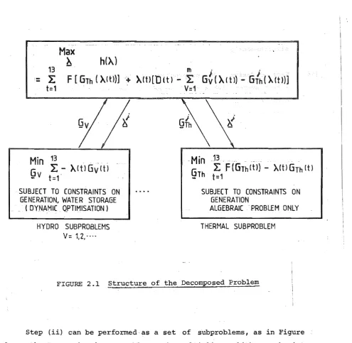
FIGURE 2.1 structure of the Decomposed Problem
Step (ii) can be performed· as a set of subproblems, as in Figure
2.1, as the Lagrangian is separable. The multipliers, A(t), can be inter~
preted as incremental costs of generation, or "price". The thermal
sub-problem is simple - generation with incremental cost less than or equal to
A(t) is operated. Hydro generation is more difficult. These subproblems,
finding the optimal G (t) sequence for the given A(t) set handed down by
v
the co-ordinator, make up the bulk of the work in f;nding the solution.
To summarise, the subproblems are solved with a given set of
incre-mental costs, producing generation schedules. The co-ordinator looks at
the total generation for each time interval, then adjusts A(t) upwards to
increase generation if the total is less than demand, or vice versa. When
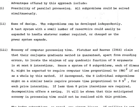
[image:32.563.51.547.45.528.2]Advantages offered by this approach include:
(i) possibility of parallel processing. All subproblems could be solved
simultaneously.
(ii) Ease of design. The subproblems can be developed independently.
A test system with
a
small number of reservoirs could easily be expanded to handle whatever number required, or changed as thepower system expands.
(iii) Economy of computer processing time. Fletcher and Reeves (1964) claim
that their conjugate gradients method is guaranteed, apart from rounding
errors, to locate the minimum of any quadratic function of N arguments
in at most N interations. Hence a system of 8 subproblems, each of dimension
N, might be expected to require computer time proportional to (BN)2 if solved as a whole by this method. If decomposed, the 8 individual subproblems
. 2
might on a similar basis require prOCeSs time proportional to 8 N , for
each price interation. If less than 8 price iterations are required, decomposition offers a saving. It will be shown that this anticipated
economy in processing time could not be realised with this problem.
The hydro subproblems, as posed, are almost linear. If spilling is not permitted, or does not occur, they are linear. As a result, if. A (t
l)
=
then Gv(tl ) and Gv(t2) might be able to take on a whole range of values giving
the same subproblem cost, i.e. increasing Gv(t
l) while decreasing Gv(t2) by the
same amount will have no effect on subproblem v cost, but will affect ~(~(t) ),
the co-ordination problem. This is because the demand/generation mismatch will
[image:33.563.56.539.69.442.2]be affected.
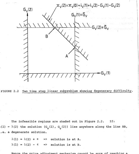
Figure 2.2 shows this difficulty fora simp~e two time step subproblem. The cost to be minimised is:
where x (0), x (2) are given
v
v
x (1)
=
x (0) + i (l)-G (1)v v v v
x (2)
=
x (1) + i (2)-G (2)v v v v
o ~ G (y) ~
G
v
v
x
=
storage vi == inflow v
FIGURE 2.2 Two time step linear subproblem showing degeneracy difficulty.
The infeasible regions are shaded out in Figure 2.2. If:
"(1) ; : "(2) the solution (G (1), G (2» lies anywhere along the line AB,
v v
i.e. a degenerate solution.
"(1)
=
"(2)+
€ => solution is at A. "(1)=
"(2)-
€ => solution is at B.Hence the price adjustment mechanism cannot be sure of reaching a
solution as the solution might be a specific point between A and B.
Introducing a non-linearity, such as quadratic transmission losses, would
put a curve into the cost function, eqn (2.6). As this is only a small
effect, the curvature would not be great, and convergence is ··likely to be
slow or unreliable. Losses also result in (relatively
between subsystems, with non-zero off diagonal terms in
weak) coupling
a
2Fy 2 • [image:34.563.51.520.53.572.2]From Lasdon (1970), the method will, in general, converge if ~(~ *(t) is differentiable, where. ~* (t) is the value of A (t) at the solution. One of the conditions for differentiability is that F(G
Th (t) ) be strictly convex. Straight lines define only a convex region, so the optima~ A*(t) does not
necessarily give the optimal releases, G (t).
v
Lasdon also points out that linear subsystems can only arrive at activity
levels which are extreme points of their constraint sets. The optimal activity
levels of the overall system may be interior to the sub-system constraints and
only by weighting the various extreme points can these interior points be generated.
So complete decomposition of a linear system is not possible. Dantzig-Wolfe
solution by decomposition of linear programs is actually only partial decomposition,
functioning in the manner outlined by Lasdon, above, i.e. the co-ordination level
weights subsystem solutions.
As the problem is almost linear, it was found that the expected square
relationship between problem dimension and computer time does not apply. The model
described in Chapter 3 has non-linearities due to the spilling of excess water, and
quadratic transmission line losses. Three and eight reservoir models have been
solved (neither using decomposition), by the same conjugate gradients method. The
eight reservoir problem required about l5% more function evaluations than the three
reservoir version. Hence processing time is approximately proportional to problem
dimension, and the square relationship mentioned earlier does not apply. This
indicates that each price interation of a decomposed problem would require as
much computer time as the complete solution without decomposition.
Difficulties caused by the "nearly linear" nature of the problem led to the
rejection of the decomposition approach. The lack of any savings in computer time
did not become evident until much later. Modelling transmission losses produces
some curvature in the sub-problem objective functions, but this is only a small
effect. It appeared to be insuffici~nt to prevent small changes in price from
one iteration to the next causing switching from one corner point to another
(as for the completely linear case). As a result, attention turned to the method
of Chapter 3, solving one large non-linear progra~ by a reliable conjugate
2.6 CONCLUSIONS
The methods reviewed generally fell into four groups:
(i) Deterministic, excessively simple problems, so the method is unproved
or inapplicable for large, realistically complicated systems.
(ii) Deterministic, realistic models, with the potential to assist power
system operating organisations to varying extents.
(iii) Stochastic one reservoir models giving a true stochastic solution
for that model, but not applicable to multi-reservoir pystems.
(iv) Multi-reservoir stochastic methods neglecting various aspects such
as transmission losses, or some non-linear effects, or only crudely
approximating stochastic inflows.
Experience with the decomposition method of section 2.5 led to the
choice of a single large nonlinear programming solution technique as most
likely to succeed. Also, the non-linear programming approach is the least
restrictive on the model, of the methods considered. Decomposition was
considered likely to be unreliable, have greater difficulty in handling
coupling between reservoirs (non-separable benefits), and to have, at besti
advantages that are declining in significance as computers become more
CHAPTER 3
OUTLINE OF A GENERAL MODELLING AND SOLUTION TECHNIQUE
FOR RESERVOIR SCHEDULING
3.1 INTRODUCTION
In Chapter 2 various possible approaches to hydro-thermal scheduling
were discussed. It was concluded that a mathematical programming method
was most likely to succeed. A generalised description of the deterministic
hydro thermal scheduling model will be given in this chapter. Chapter 5
presents the application of these principles to the New Zealand power system,
and includes extensions to handle a D.C. link.
The algorithm is designed for use over a one year time horizon, with
a time step of from one to four weeks.
Modelling of physical components of the power system will be described
first, including details of the development of the D.C. loadflow loss
coeff-icients. The means of converting a general time dependent problem into a
static equivalent by forming a Hamiltonian follows. Then this method is
applied to the model, constraint enforcement described, and gradient
cal-CUlations given. The result is a set of equations suitable for solution
by an unconstrained static hill climbing algorithm. Chapter 4 describes
the conjugate gradients method used to do this.
Throughout the model development the most simplifying assumptions
possible have been made, unless there is a good reason for doing otherwise.
Only those components of the power system likely to be limiting
factors need be modelled. If some factor is not thought to be worth
considering by those involved in the present planning methods, then it is
likely not to be worth including in the model. If well designed,the power
system will not be limited in its performance by, for example, the rating
of a single transformer at some substation, so there is no need for it to
The level of model detail must be consistent with the time scale
of the problem. It is not possible to ensure that all components of the
system will always be within their normal operating range when dealing
with a one week time step as the exact load pattern is not known, nor
could it be modelled. Also, there is no point in devising a model so
complicated that it can not be solved.
Consequently transmission system constraints have not been modelled,
but constraints on power transfer between two regions can be incorporated,
as is done for the New Zealand example. Transmission losses are modelled
by the D.C. loadflow loss coefficients calculated before the optimisation
commences. Losses are thereafter calculated from the generator outputs
and these coefficients only.
All thermal stations and large reservoirs are modelled individually.
Reservoirs in series are possible, and uncontrollable tributary inflows
can be handled. Run-of-river hydro stations are modelled with little
effort. Constraints on reservoir levels, reservoir releases, and
gener-ation can be enforced, and may be time varying.
3.2 DEMAND
Power demand and other time-dependent quantities are expressed as
average values over discrete time intervals. One week is likely to be
the most convenient interval in practice, as loads have a weekly cycle.
Short duration peaks often require the use of higher co~t thermal stations
than consideration of average weekly energy requirements would suggest.
Some means of representing load fluctuation during each week is needed.
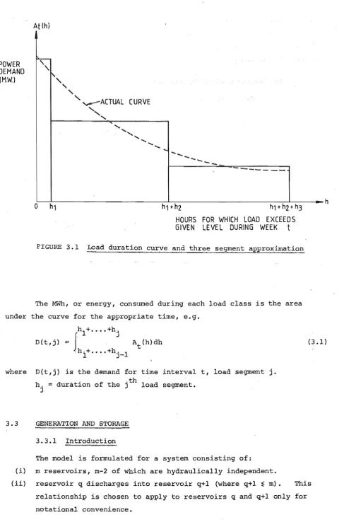
Figure 3.1 is a load duration curve, giving the demand At(h) in MW
which is exceeded for h hours, in week t. This curve is approximated by
~ load classes. (~=3 for example of Chapter 5). The load classes can, and will usually, be selected to be of different durations. The peak
load segment might be made shorter than the others to ensure that the
weekly maxima are represented well, as these can require very expensive
. POWER 'DEMAND
IM'w)
Atlhl
~
\
r--.,
"
"
,
...-ACTUAL CURVE
"
,
[image:40.563.38.526.31.770.2]...
,
...
,
... ...
...
o
...
-
----h1 + h2
HOURS GIVEN
--
...---h1 + h2 + h3
FOR WHICH LOAD EXCEEDS
LEVEL DURING WEEK
t
FIGURE 3.1 Load duration curve and three segment approximation
The MWh, or energy, consumed during each load class is the area under the curve for the appropriate time, e.g.
h
D(t,j) (3.1)
where D(t,j) is the demand for time interval t, load segment j.
h
j = duration of the jth load segment.
3.3 GENERATION AND STORAGE
3.3.1 Introduction
The model is formulated for a system consisting of:
(i) m reservoirs, m-2 of which are hydraulically independent.
(ii) reservoir q discharges into reservoir q+l (where q+l ~ m). This
relationship is chosen to apply to reservoirs q and q+l only for
(iii) n-m thermal stations.
(iv) p run of river stations.
(v) 52 time intervals (weeks).
(vi) ~ load segments.
The indices used in various summations include:
v indexing reservoirs and thermal stations,
t indexing time segments,
j indexing load segments.
Specific features of each type of station follow.
3.3.2 Hydro Reservoirs
The most important assumption made in this model is that all hydro
stations fed by a given long term reservoir, but upstream from the next
long term reservoir if it exists, can be lumped into one equivalent station.
It is a~sumed that the individual scheduling of stations, from an aggregated
figure, can be done without upsetting the long term schedule significantly.
This process would require another optimisation with a shorter time scale.
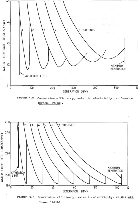
Generation at a hydro station is a function of head, flow rate, and
tail water elevation. Figures 3.2 and 3.3 show how the water to electrical
power conversion factor (in CUSECS/MW) varies with generation for Benmore
and Waitaki stations. The various curves are for when all machines actually
in use are equally loaded, as this gives the most efficient operation by the
equal incremental cost principle.
Clearly these characteristics are impossible to model for weekly
outputs as the exact loadings on each station are not known - only the
average output of the whole chain of stations over each load segment. Even
when a reservoir feeds only one station, the fact that average, not
instant-aneous, loadings are calculated by the scheduling algorithm prevents the
use of exact conversion factors.
Head variations are only known for stations drawing water directly
from their long term storage reservoir. At other stations head effects
can not be modelled, as the variations are unknown.
Using the available information, some approximations must be made.
Here, head effects have been neglected, and constant water to electrical
energy conversion factors have been used.
simplification. So:
45r---y---.----.---.--~~--,---~
-
U'l u w U'l ::> uw 43
~
0::
:3
9
u...~ 42
I -<t :3 250 240
-U'l u w U'l ::> u 220 w I -<t 0:: 3: 0 ....J u... 0:: w I-~
190 06 MACHINES
'CAVITATION LIMIT
100 200 300 400
. GENERATION 1M W)
/ '
MAXIMUM GENERATION
500
FIGURE 3.2 Conversion efficiency, water to electricity, at Benrnore
(Green, 1971b).
20 40
7 MACHINES
60
GENERATION (M W)
80
MAXIMUM GENERATION
'"
100 110
FIGURE 3.3 Conversion efficiency, water to electricity, at Waitaki
(Green 1971b).
[image:42.564.45.527.58.769.2] [image:42.564.54.533.58.411.2]R =.K x volume of water released
v v
where: R is the energy generated, in MWh, by all stations in a river v
system,
K is the constant conversion factor, v
v
E [}.,m]
(3.2)
Water can now always be expressed in terms of its. generation potential in MWh.
A further simplification is that leakage and evaporation losses from large storage reservoirs need not be considered in most cases. This is because lake inflows are measured by recording lake level and outflow.
No other method is practical for a large lake with many small rivers flowing into it. Hence the lake's losses do not appear at all, being automatically subtracted from inflows. This will be an accurate result if the surface area of the lake does not change too much with its level.
The water storage equation for all lakes except q+l, with all quantities expressed as their electrical equivalents in MWhis:
and
x
(t+l) vG (t,j) v
x
(t)-v R v (t,j) + I (t) - S (t) v v
= R (t,j) + T (t)
v v ~
I
i=l h· l.
where X (t)
=
storage in lake v at beginning of time interval t. vR (t,j)
=
release from lake during time t for load segment j. vI (t)
=
storable inflow. vs
(t)=
spill.v
G (t,j)
=
generation from all stations fed by the reservoir.v
T (t)
=
tributary flows, non storable, but may be non-existantv
for some reservoirs.
h.
=
duration of load segment j (hours).J
Spill is calculated from
(3.3)
S (t)
=
vx
v 0 Jl,(t)
-
1:
j=lif
otherwise
R (t,j) v
X (t) v
+ I (t)
-
X(t) vJl,
1:
R (t,j) + I (t) >X
(t)j=l v v v
(3.5)
i.e. lake levels are simply clipped off at their maximum values, the excess
being "spill". This strategy is in contrast to the approach of, for
example, Dillon (1974) who applies a penalty to minimise spill.
is justified in section 3.6.5.
OUr strategy
Constraints on the variables of eqns (3.3) and (3.4) must be enforced.
Lower limits on storage exist.
x
(t) ::: X (t)-v
v
where X (t)
=
minimum storage, which may be time varying.-v
Limits on generation are:
G -v (t,j) ~ G v (t,j) ~ G (t ') v ,J where G (t,j) = minimum generation,
-v
G··(t,j)· == maximum generation,
v
and for reservoir releases:
R (t,j) ~ R (t,j) ~
R
(t,j)-v v v
where R ·(t,j) == minimum release,
-v
R (t,j)
=
maximum release. v(3.6)
(3.7)
(3.8)
The releases, R v (t,j), are the control variables in this model, so .
restrictions on generations, G (t,j), must be converted into constraints on v
R (t,j) for the optimisation procedure.
v The state (dependent) variables
are reservoir storages.
Tributary flows are assumed to occur uniformly over the whole of
each time interval. The limited storage behind individual dams is assumed
to be sufficient to smooth out fluctuations over a time interval. Spilling
of tributary flows is allowed only when they are so high that generation
limits are exceeded with minimum permitted controllable releases, i.e.
G (t,j) ... R (t,j)
v -v
i f T (t) v h. J ~
L
i=l h. ~> G (t,j) - R (t,j) for any j.
Tributary flows are considered to be fully utilised otherwise, imposing a
restriction on the minimum possible generation:
h. G (t,j) ~ T (t)
-v
v
-.II----
x, J,-- +: R ( -v t , j )L
i==lh.
J.
Maximum reservoir releases are also restricted - they can not exceed
generation capacity remaining after tributary flows have been utilised:
R
(t,j) ~G
(t,j) - T (t)v v v
h.
)
i=l h.
].
For the lower reservoir of the cascaded pair of reservoirs only
equation (3.3) need be changed:
$/.,
Xn+l(t+l) = Xn+l(t). -
L
R l(t,j) + I 1 (t) - S 1 (t)~ ~ j=l q+ q+ q+
(3.10)
(3.11)
(3.12)
where k
I
1 converts generation from stations fed by reservoir q to give q q+the generation potential of the water they have used when it flows into
reservoir q+l.
Equation (3.12) assumes that the spill S (t) is lost completely, q
but the equation could be modified so that spill also. goes into reservoir q+l.
The time delay of flow from one reservoir to the next is neglected - valid
if it is much less than a week.
3.3.3 Run-of-River Hydro
Any hydro station with only short term stor,age facilities, or any
other station for which output can be predetermined is treated in a very
simple way. This category can include for example geothermal stations,
which have zero marginal cost, and so will be operated whenever available.
The output of these stations is treated as negative demand. Total
run of river output is therefore subtracted from total demand figures for
each time and load segment. When calculating loss coefficients, their