3D modelling using partial differential equations (PDEs).
OSMAN, Abdusslam.
Available from Sheffield Hallam University Research Archive (SHURA) at:
http://shura.shu.ac.uk/20153/
This document is the author deposited version. You are advised to consult the
publisher's version if you wish to cite from it.
Published version
OSMAN, Abdusslam. (2014). 3D modelling using partial differential equations
(PDEs). Doctoral, Sheffield Hallam University (United Kingdom)..
Copyright and re-use policy
Sheffield Hallam University Learning and Information Services
Adsetts Centre, City Campus Sheffield S1 1WD
ProQuest Number: 10697460
All rights reserved
INFORMATION TO ALL USERS
The quality of this reproduction is dependent upon the quality of the copy submitted.
In the unlikely event that the author did not send a com plete manuscript and there are missing pages, these will be noted. Also, if material had to be removed,
a note will indicate the deletion.
uest
ProQuest 10697460
Published by ProQuest LLC(2017). Copyright of the Dissertation is held by the Author.
All rights reserved.
This work is protected against unauthorized copying under Title 17, United States C ode Microform Edition © ProQuest LLC.
ProQuest LLC.
789 East Eisenhower Parkway P.O. Box 1346
3D Modelling Using Partial Differential
Equations (PDEs)
Abdusslam Osman
A thesis submitted in partial fulfilment of the requirements of Sheffield Hallam University
for the degree of Doctor of Philosophy
Table of Contents
List of Figures v
List of Tables vii
Abstract xi
Acknowledgements xii
1 Introduction 1
1.1 Scope of the Research... 1
1.2 Background and Motivation ... 3
1.3 Aims and O b je c tiv e s... 8
1.4 Contributions to K n o w led g e... 9
1.5 Thesis O rganisation... 9
2 The Related Work 11 2.1 Introduction... 11
2.2 3D Representation ... 11
2.3 Compression ... 13
2.5 D iscussion... 19
3 Partial Differential Equations and their Solutions 21 3.1 Introduction to Partial Differential Equations ... 21
3.2 Boundary Value P ro b lem ... 24
3.3 Classic Fourier S e rie s... 25
3.4 Dirichlet Boundary for Laplace’s Equation... 27
3.4.1 The solution by separation of variables ... 27
3.4.2 The solution by the method of l i n e s ... 30
3.5 Signal Representation... 33
3.5.1 The Discrete Fourier Transform (DFT) ... 34
3.5.2 The Discrete Cosine Transform (DCT) ... 36
3.5.3 The Discrete Wavelet Transform (D W T)... 36
3.5.4 The PDE-based A p p ro a c h ... 38
3.6 Interpolation and C om pression... 39
3.7 3D Geometry Formats ... 40
3.8 D iscussion... 43
4 Data Modelling and Pre-Processing 45 4.1 Introduction... 45
4.2 Data Representation... 46
4.3 Creating Scattered Interpolation P o in ts... 48
4.4 M odelling... 51
4.5 M e th o d ... 53
4.5.1 Polygon Reduction by Explicit Structured Vertices . . . . 53
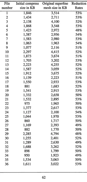
4.6 Discussion 61
5 Efficient 3D Data Compression Through Parameterization of
Free-Form Surface Patches 66
5.1 Introduction... 66
5.2 Polynomial Interpolation... 67
5.3 R esults... 72
5.3.1 Data Compression by P o ly n o m ial... 72
5.3.2 3D R econstruction... 74
5.3.3 Evaluating the F i t ... 76
5.4 D iscussion... 78
6 Partial Differential Equations for 3D Data Compression and Recon struction 80 6.1 Introduction... 80
6.2 M e th o d ... 81
6.2.1 Data P rep aratio n ... 81
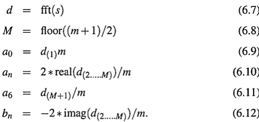
6.2.2 Fourier Series A pproxim ation... 82
6.2.3 PDE M odelling... 86
6.3 Experimental R e su lts... 90
6.4 Assessing the Quality of 3D R econstruction... 92
6.5 Discussion... 95
7.2 M e th o d ... 98
7.2.1 The DFT M eth o d ... 98
7.2.2 The DCT M ethod... 99
7.2.3 The DWT M e th o d ... 101
7.3 Experimental Data ... 104
7.4 R esults... I l l 7.4.1 DFT, DCT and DWT Applied to Vertices Lying in a Sin gle P l a n e ...I l l 7.4.2 Extending DFT, DCT and DWT to Multiple Planes . . . . 114
7.5 D iscussion...124
8 Conclusions and Further Work 126 8.1 S u m m a ry ...126
8.2 C onclusions... 129
8.3 Future W o rk ... 131
References 133
Appendix A Published papers 152
List of Figures
3.1 Defining Laplace’s equation over a rectangular domain... 28
3.2 The given boundary c o n d itio n ... 31
4.1 The GMPR scanner maps light planes hitting the target to surface points (x,y,z)... 48
4.2 The implicit triangulation method between two planes • • • 49 4.3 Connected path of triangulation mesh... 50
4.4 Textured and shaded 3D m o d e l... 53
4.5 Sampling points on a regular g rid ... 54
4.6 The bounding box and structured cutting planes... 56
4.7 Original 3D m e s h ... 58
4.8 Horizontal p la n e s ... 58
4.9 Vertical planes... 59
4.10 The intersection points of each horizontal and vertical plane . . . 59
5.1 Polygonal mesh detail... 67
5.2 Polynomial interpolation along cutting p la n e s ... 70
5.3 Polynomial interpolation of degree 3 ... 72
5.5 Polynomial interpolation degree 20 to 4 0 ... 75
5.6 Polynomial interpolation degree 8 0 ... 75
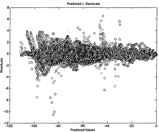
5.7 Scatter plot of Predicted Values against R esid u als... 77
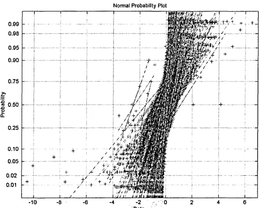
5.8 The normal-probability plot of the re sid u a ls... 78
6.1 The illustration of PDEs compression and reconstruction... 82
6.2 Rectangular domain for solving Laplace’s equation... 87
6.3 The effects of iteration steps on convergence... 89
6.4 Left: original superfine meshes; right: PDE reconstructed 91 6.5 Visualisation of the error su rfa c e ... 94
6.6 Scatter plot of Predicted Values against R esid u als... 94
7.1 Example of a textured and colour map 3D model ...104
7.2 The 3D model used for illustration of compression techniques. . . I l l 7.3 DFT and DCT reconstruction... 112
7.4 DWT 3-level decomposition and reconstruction... 113
7.5 Reconstructed models quality Q = 1 0 0 ...115
7.6 Reconstructed models quality <2 — 5 0 ...116
7.7 PDE based reconstruction quality Q = 1 0 0 ... 117
7.8 PDE based reconstruction quality Q = 5 0 ...118
7.9 Average RMSE errors ...118
List of Tables
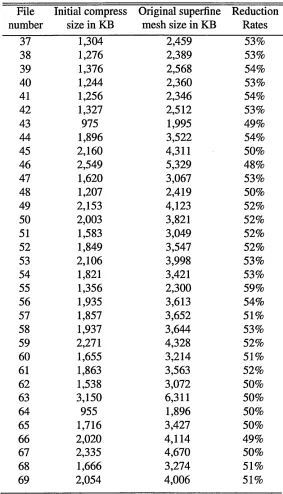
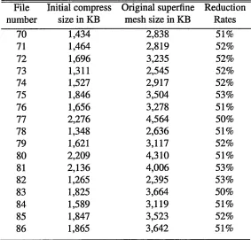
4.1 Initial compression by re-meshing operation... 62
4.2 Initial compression by re-meshing operation... 63
4.3 Initial compression by re-meshing operation... 64
5.1 Compression rates in percentage... 74
5.2 Trend of increasing R2 ... 78
6.1 Text file format for 3D compression using D F T ... 85
7.1 Text file format for 3D compression using D C T ...100
7.2 Text file format for 3D compression using D W T ...103
7.3 Data files experiments 1 ...105
7.4 Data files experiments 2 ...106
7.5 Data files experiments 3 ...107
7.6 Load and display PDE data 1 ...108
7.7 Load and display PDE data 2 ...109
7.8 Load and display PDE data 3 ...110
7.9 Compressed data files and CPU tim e ... 121
7.10 Compressed data files and CPU tim e ... 122
Acronyms & Abbreviations
API Application programming interface
ASCII American Standard Code for Information Interchange
B-spline Basis spline
CAD Computer aided design
CAM Computer Aided Manufacturing
COLLADA COLLAborative Design Activity
CPU Central Processing Unit
DCT Discrete Cosine Transform
DE Differential Equation
DFT Discreate Fourier Transform
DWT Discrete Wavelet Transform
DirectX A collection of application programming interfaces (APIs)
EB Exabytes
EBCDIC Extended Binary Coded Decimal Interchange Code
FDM Finite Difference Method
FEM Finite Element Method
FFT Fast Fourier Transform
FWT Fast Wavelet Transform
HPF High pass filtration
HTML HyperText Markup Language
JPEG Joint Photographic Expert Group
JSON Java Script Object Notation
Java3D 3D application programming interface for the Java platform
LPF Low pass filtration
MLS The moving least squares
MOL The method of lines
MPEG-4 Moving Picture Experts Group
Matlab Matrix laboratory
NURBS Non-uniform rational basis spline
OBJ An object file
ODE Ordinary Differential Equation
OpenGL ARB The OpenGL Architecture Review Board
PB Petabytes
PC Personal Computer
PDE Partial Differential Equation
QoS Quality of Service
R2 Coefficient of determination
RAM Random access Memory
SSE Sum of Squared Errors of Prediction
SST Total Sum of Squares
VRML Virtual Reality Modeling Language
XML Extensible Markup Language
iDCT Inverse Discrete Cosine Transform
iDWT Inverse Discrete Wavelet Transform
Abstract
Acknowledgements
The successful completion of this study would not have been possible without the involvement of a number of people and institutions. First, I wish to acknowledge my sincere gratitude to my supervisor, Professor Marcos Rodrigues. His keen enthusiasms for work and constant good humoured spirits have been a source of encouragement to me. His comments and criticisms have been appreciated as much as his learned guidance and advice during the past three years of study and preparation of this thesis.
Second, I would like to sincerely thank my examiners, Dr. Leonardo Bottaci and Dr. David Cooper, for their valuable comments, and for raising interesting points in their report, leading to improvements in this thesis.
Third, I gratefully acknowledge the financial support provided by the Libyan higher education, and Sheffield Hallam University for granting me the opportunity to pursue the Doctor of Philosophy Degree in this institution.
Forth, there is a long list of people who provided help and support. It is impos sible to mention all of them, but my special thanks go to my second supervisor Dr Alan Robinson, Prof Ann Macaskill, Tracey Holmes, and all colleagues from the GMPR research group for their guidance and support. To all those who supported me in one way or another but have not been mentioned individually, please accept my gratitude.
Chapter 1
Introduction
1.1 Scope of the Research
Within three dimensional computer graphics, 3D modelling is the process of cre ating the numerical rendering from the three-dimensional surface or volumetric/- solid representation of the object via specialised software. Models could be shown like a two-dimensional image via a course of action referred to as 3d render or even used in your personal computer simulation associated with actual phenom ena. Such graphical models (a surface or volumetric) are normally designed and constructed using CAD-Computer Aided Design software or acquired through 3D scanners. Once defined in an appropriate format, any 3D model can be printed out using specialised 3D printing devices. This thesis is only concerned with 3D sur face data; in particular, surface patches defined on a regular xy-grid where the depth of each point is defined in the z-axis. Such surface patches are typical of data acquired using conventional 3D scanners based on stereo system perspective, structured light or time-of-flight techniques.
while lossless means no loss of information. This research only describes lossy compression. Data uncompressing is the process of recovering the original data from the compressed data and normally this is achieved by reversing each step of the process of the compression algorithm. When one refers to compression it normally means both the process of compression and uncompressing. Unless specifically stated otherwise, this thesis uses the word ‘compression’ in this con text.
The research approach to 3D compression described in this thesis follows four steps:
1. To investigate a method to define structured geometric information;
2. To investigate polynomial interpolation techniques;
3. To investigate the use of partial differential equations; and
4. To perform comparative analyses with related data compression techniques applied to the 3D case, such as Discrete Fourier, Wavelet, and Cosine trans forms.
In the techniques proposed in this dissertation, first, a polygon reduction described in Chapter 4 is applied to the mesh resulting in a set of vertices lying in structured planes of a sparse, regular grid. The data defined on such grids with their prac tical implementation issues and incorporation into compression techniques are discussed in Chapters 5-7.
The first approach to compression described in Chapter 5 is by using polyno mial interpolation. The technique is applied to surface patches and it is shown to be capable of decreasing the mesh by more than 99%. However, there are some limitations such as lack of precision, and for polynomials of higher degree the 3D surface becomes unstable and with smaller compression rates.
methods are tested in various experimental setups and their effectiveness is evalu ated and discussed.
In Chapter 7 new methods for 3D data compression and reconstruction are proposed and demonstrated. Upon applying a method of polygon reduction, the vectors describing the data are parametrically defined and a comparative analysis is presented via the Discrete Fourier Transform (DFT), Discrete Cosine Trans form (DCT) and Discrete Wavelet Transform (DWT). The transform coefficients are further processed according to a quality factor, which substantially decreases the amount of data. The file formats are defined with the necessary parameters for a full reconstruction of the sparse mesh. Finally, in order to recover the vertex density of the original mesh, the reconstructed data are represented by elliptic Par tial Differential Equations (PDE) and iteratively solved between adjacent planes in connection with the Laplace equation. Experiments demonstrate the effective ness of the methods allowing compression rates of over 98% compared to the OBJ file format and over 91% compared to a list of vertices in ASCII format.
1.2 Background and Motivation
Current improvements in three dimensional modelling have led to a common num ber of applications in most areas of science and engineering. Three dimensional objects are now widely used in applications such as games, mechanical and archi tectural design, archaeology, as well as medical engineering among others. The actual common integration associated with 3D models in different fields motivates the need to be able to store, list, classify, and recover 3D objects automatically and efficiently.
to share CAD/CAM models with e-commerce clients, to upgrade material with regard to entertainment applications, or to support collaborative design, research, and show of technological innovation as well as scientific data sets. Bandwidth limitations and storage space restrict the transmission and use of 3D data over the network.
Data compression techniques tend to be centred on representing the actual geometry and connectivity of the vertices in the triangulated mesh. There has been no systematic approach to the geometric parameterization associated with arbitrary 3D objects aiming at efficient representation and compression. As a result, a major concern of this research is to define the possibilities associated with the compression of 3D data for fast transmission over the Internet, without lack of precision and performance.
To achieve this, the thesis involves both theoretical and practical work. The main theoretical work involves the development of mathematical methods for effi cient representation and parameterization of PDE-based models as well as geom etry optimisation methods for efficient fitting of PDE models to data and efficient encoding of the residuals. This really is achieved by solving a second order, ellip tic PDE uses the method of lines to generate a surface from the solution to those equations. Practical work involves the implementation of the methods within the software; what is addressed here is 3D compression by a number of methods and techniques, which is subject to experimentation regarding overall performance and stability.
which is explored in this study involves 3D facial biometric verification at airports. The method is non-intrusive and aims at minimal disruption. It is based on our past experience with 3D biometrics at Heathrow Airport (London, UK) in 2005. In this scenario, an enrolment shot is taken and reconstructed in 3D at an automated check-in desk, where a new database is created for each flight. At the gate before boarding the plane another 3D shot is taken for verification.
The created databases are transmitted to the local Police who perform a search against their records. If the Police find no information to warrant keeping the data for longer, all data must be erased after a time lapse, normally within 24 hours. For international flights and where no mechanisms for sharing information between Police Forces are available, the data can be transmitted to the destination
Police authorities before the flight actually arrives at the destination. A significant
constraint of this scenario is that 3D files are very large; a high definition 3D model of a person’s face is around 20MB. For a flight with 400 passengers, this would mean dispatching 8GB of data. If one considers the number of daily flights in a medium sized airport, it can be concluded that this may be unworkable. It is clear that methods to compress 3D data would be beneficial to the scenario considered here but, more importantly, would represent an enabling technology for a large number of other potential applications. For instance, the application of simple texture mapping would lead to the creation of naturally-looking facial images, but on the other hand, conceal the individuality of the subject in the 3D face geometry. Apart from the aspects of privacy, confidentiality, and security concerns, the point being made here is that without data compression it is impossible to make such a scheme work. About 70 million passengers go through London Heathrow per year, almost 200,000 per day. Each high density facial scan takes about 20MB of disk space, so one would be contemplating about 4TB (terabytes) of data per day and 1.4PB (petabytes) per year. To dispatch such a vast amount of data over the network to the local police station and potentially to the origin and destination police authorities is unworkable with current technologies.
Internet. In general, there are three methods one can use to share 3D data. The first method is based on image compression where each snapshot of a 3D scene is compressed as a 2D image. The second method is based on hierarchical im provement of a 3D structure with regard to transmission, where a coarse mesh is followed by increasing refinements until the original, full 3D model is recon structed in the other end. The third method is based on mesh compression where algorithms traverse the mesh for a local compression of polygonal relationships.
The principle of compression proposed here is inspired by the GMPR scanning method and its resulting mesh properties. The first step described in Chapter 4 is to cut an arbitrary triangulated mesh with a suitable number of horizontal and vertical cutting planes and detect the intersection point of such planes on the mesh. In order to code the mesh, the (x,y) coordinates are directly given by
the distances between the planes, so there is no need to code any (x,y) values
explicitly. Only the z-values are subject to compression schemes. The method is
not lossless and this research investigates compression techniques for the z- values
based on polynomial interpolation and also using PDEs for surface reconstruction. Therefore, for a generic surface path the method involves cutting a number of planes parallel to the y-axis (or X-axis) of the 3D unconstrained point cloud; then for each plane, finding the points in the structure intercepted by each plane (within a threshold). In this way, an equivalent scan line structure as in the GMPR scanning method is obtained.
This thesis investigates new methodologies on geometric coding of single value functions where the connectivity is explicitly derived from geometry. Meth ods for single-value functions are demonstrated in Chapter 5 where connectivity is not coded at all. Once the geometry is coded, compressions over 99% are achieved through the method of re-meshing the structure and representing the (;t,y,z), in parametric form using polynomial interpolation.
models are proposed in a way rather different from the previous work on polyno mial interpolation highlighted above. Here it is proposed to represent the geome try and connectivity of the mesh by means of solving an elliptic PDE. A perceived advantage of the PDE-based approach is that it defines shapes by means of data distributed around the shape boundaries and feature points only. This approach contrasts with mesh models and spline surfaces, which often require hundreds of control points in order to represent a realistic object. However, it is noted that to date there has been no systematic approach to the geometric parameterization of arbitrary 3D objects aiming at efficient representation and compression.
The main idea is to compress the geometry of each (sparse) cutting plane sep arately using either Fourier, Discrete Cosine or Discrete Wavelet transforms. And then on the uncompressing stage, use each pair of such planes in turn as boundary conditions for an elliptic PDE and iteratively solve the Laplace equation between the boundaries by the method of lines. The connectivity of the mesh is directly de rived from solutions to the Laplace equations and the boundary planes. Therefore, information on the number of vertices as well as a scale of the surface together with the set of points lying in each cutting plane are integral components of the PDE parameters. Cutting planes are used as boundary conditions and there is no dependency on time.
approximation error distance of different methods.
1.3 Aims and Objectives
The aims of research are to demonstrate that PDE based modelling with geometry re-meshing operations can effectively be used for 3D data compression of mesh geometry and connectivity. The approach is different from current methods that are based on coding, connectivity having geometry as a dependent property; the proposed methods are based on geometry coding with connectivity derived from geometry.
The objectives are identified as follows for arbitrary surface patches:
• To define a re-meshing method for efficient geometry coding through mesh cutting planes in ZY-directions.
• To define the possibilities associated with the compression of 3D data for fast transmission over the Internet. Assuming that effective compression can be achieved, would the proposed scheme yield satisfactory results?
• To collect statistics on the bit rate of such representation and compare with existing polynomial as defined in [Rodrigues et al., 2010], and related work in the literature.
• To investigate and define methods for PDE representation of plane intersec tions using Laplace and Fourier spaces and alternative representations.
• To define an optimal method for PDE representation from the results of the investigation.
Given an arbitrary surface patch, the proposed method is based on determining the mesh intersection of structured cutting planes in horizontal and vertical directions.
Each intersection point is a vertex defined on a regular xy-grid where the z-value
proposed is an interpolation of the z- values by high degree polynomials. Second, a method is proposed for Fourier based data compression and PDE based data uncompression. Finally, a comparative analysis of the PDE method is presented via the DFT, DCT and DWT methods.
1.4 Contributions to Knowledge
This thesis presents a novel approach to accurate, efficient representation and compression of 3D data compression centred on the parameterization of surface patches. The major contributions made by this work are as follows:
• In the first approach using interpolation of polynomials of high degree from 30 to 80 degrees, the result shows a mesh reduction of over 99% compared to the OBJ file format.
• A new approach was taken for 3D compression and reconstruction using the method of lines to solve elliptic PDE, achieving a compression rate of over 98% compared to the OBJ file format. The methods are based on DFT to reconstruct the original data from the vertices lying in each plane. Theoret ical results, in addition to numerical illustrations indicate the superiority of this method, compared to the previous approaches used so far.
• The thesis provides a comparative analysis of DFT, DCT, and DWT in con nection with PDEs to recover the full vertex density of the original mesh. Results indicate that both DCT and DWT are more robust than DFT for compressing the data mesh.
1.5 Thesis Organisation
1. Chapter 2 presents an overview of related work, with the history of the numerical analysis using different methods of solving the PDEs.
2. Chapter 3 introduces the basic concepts of Partial Differential Equations and their solution. Direct methods and iterative methods are formulated, and their feasibility is considered.
3. Chapter 4 presents the data modelling and the pre-processing to be used in all experiments in the thesis. This is the first step of the compression method.
4. Chapter 5 presents a polynomial interpolation method for efficient 3D data compression through parameterization of free-form surface patches.
5. Chapter 6 introduces Partial Differential Equations for 3D data compression and reconstruction. The focus of this cFhapter is on data interpolation using the Fourier Transform.
6. Chapter 7 describes a comparative analysis of data compression via the Fourier Transform, Discrete Cosine Transform, Discrete Wavelet Transform and Partial Differential Equations.
Chapter 2
The Related Work
2.1 Introduction
In this chapter, an overview is provided of research work with the relevant back ground related to the work presented in the thesis. It is beyond the scope of this thesis to give a comprehensive overview of all related work. Thus, this chapter will concentrate mainly on research closely related to the work presented later, categorised in groups according to the method used. The first category is 3D rep resentation, the second is compression and the third is PDE-based approaches.
2.2 3D Representation
may not define a volume degree. Solid modelling extends the actual techniques of surface modelling to deal with the representation as well as manipulation of volumes, totally surrounded by surfaces, say, for example a cube, buildings, and the human body.
There are three well-known methods to represent a model:
1. Polygonal meshes: Points in 3D space, known as vertices, are connected through a line segments to form the polygonal mesh. Most of 3D models today are built as textured polygonal models, as they are flexible and com puters can render them so rapidly. Furthermore, polygons are planar and can only estimate rounded surfaces that use many polygons [Foley, 1996; King et al., 2000]. A triangular mesh is a mesh in which all the faces are triangles. Any polygonal mesh can be transformed into a triangular mesh by triangulating each polygonal face. Even though polygonal meshes can precisely approximate any objects with planar surfaces, this approximation can be made arbitrarily close to the curved surface being modelled by using small enough polygons.
2. Curve modelling: Surfaces are defined as a curve blending control point. Curve types include splines, non-uniform rational B-splines (NURBS), pat ches and geometric primitives. These types can be given either within the implicit or parametric form. The implicit form makes it simple to deter mine if a point is actually on the surface, and if not, which side it is located. However, the implicit form will not lend itself to computing the points on the surface within a simple way, when sketching for instance and even less to local modifications of the shape. Furthermore, it is very difficult to model free-form objects using the implicit form [Akkouche and Galin, 2001; Bloo- menthal, 1988; Witkin and Heckbert, 1994].
[Catmull and Clark, 1978]. The algorithms produce a surface, which is a B-spline surface everywhere, except at a limited number of extraordinary points [Doo and Sabin, 1978].
An algorithm with one refinement step and no corner cutting was proposed in which the refinement step is used to isolate the irregularities of the mesh [Loop, 1994]. In addition, a modified Butterfly subdivision scheme, which is smooth on irregular meshes, is presented in [Zorin et al., 1996]. Subdivi sion schemes lend themselves to the representation of surfaces of arbitrary topology in addition to surfaces represented by bivariate functions [Dyn and Levin, 2002],
This dissertation is focused on polygonal meshes.
2.3 Compression
The compression schemes for geometric data models have recently been the sub ject of intensive research. Data compressions are crucial with regard to decreasing
space for storage or transfer over the network. There are two types associated with compression, the first lossy data compression, which is not guaranteed to get the same output bit for a bit for example, JPEG. Second is the lossless compression, which is guaranteed to get the same output bit for a bit at decompression example PNG, ZIP and TGZ.
coding of 30-80% which is smaller than an approach based on randomly splitting quads into triangles [King et al., 2000; Rossignac, 2001],
Other techniques for triangulated models include the work of [Shikhare et al., 2002] and vector quantization based methods [Qian et al., 1998] where rates of over 98.75% have been achieved. However, a significant drawback to this tech nique in the use of vector quantization, which adds to computation and throws valuable information away. A new compression algorithm that encodes the con nectivity of surface meshes directly into their polygonal representation, by im proving the triangulated mesh prior to data compression, is able to recover the polygons by marking the edges along with 70% compression rate [Isenburg and Snoeyink, 2000]. Some other local compression and decompression algorithms, which are sufficiently fast for real time applications, accomplished compression rates of more than 60% [Gumhold and Strafier, 1998]. Regarding geometry en coding, recently reported data compression methods for the vertex coordinates (geometry) have used vertex quantization, and geometric predictors, as well as adjustable duration encodings associated with corrective vectors in order to shrink the actual vertex coordinates [Deering, 1995; Kronrod and Gotsman, 2000; Li and Kuo, 1998; Taubin and Rossignac, 1998; Touma and Gotsman, 1998].
pression, current compression rates are still too low for general sharing of 3D geometry files over the internet. The GMPR research group has developed and demonstrated original methods and algorithms for fast 3D scanning for a number of applications with a particular focus on security [Brink et al., 2008; Robinson et al., 2004; Rodrigues and Robinson, 2010, 2011; Rodrigues et al., 2008]. The algorithms can perform 3D reconstruction in 40 milliseconds and recognition in near real-time, but saving such 3D facial models has resulted in a severe bottle neck due to the size of the data files. All data used in this research have been previously acquired using the GMPR scanner.
2.4 PDE-based Approaches
Recently, several approaches for solving PDE-based modelling have been de veloped. In particular, various methods were discussed in [Bloor and Wilson, 1997, 1989; Jain and Jain, 1978; Malcolm Bloor and Wilson, 1996; Mathews and Fink, 1994]. However, surface modelling techniques tend to be fundamental for many visual processing applications including interactive graphics, CAD/CAM, animation, and digital environments. Frequently-used representation schemes for free-form surface modelling such as spline-based approaches take advantage of simple polynomial functions in collaboration with control points [Bohm et al., 1984; de Boor, 2001; Farin, 1996; Forsey and Bartels, 1988; Piegl, 1991; Piegl and Tiller, 1987; Ugail et al., 1999]. Nevertheless, an over-all way of establish ing distinction strategies in order to determine the numerically particular quasi- linear PDE through Levenberg-Marquardt kind algorithms with regard to elliptic as well as parabolic problems may be referred to [Wiegmann and Bube, 1998]. Consequently, the problem of regularisation of the Cauchy problem for Laplace’s equation is considered to be close to the exact solution [Ang et al., 1998].
gular, finite element areas, a posteriori error estimate, adaptivity of the mesh, con forming mesh-refinement algorithms for triangulations, along with a full multi grid method for resolving linear systems [Bartels et al., 2006; Grebennikov, 2005; Rivara, 1984; Van Schijndel, 2003]. This research favours the method of lines (MOL) which is a convenient method for the numerical integration of PDEs; for example, the Korteweg-de Vries equations have been formulated to model shallow water flow [Saucez et al., 1998; Schiesser, 1994] and are solved by the method of lines.
Point datasets routinely generated via optical and photometric variety finders are usually corrupted through the noise. In order to remove these kind of deficien cies from scanned stage, clouds, a large variety of denoising approaches based on low-pass filtering are used [Linsen, 2001]. Typically, the moving least squares (MLS) surface, used for modelling and also rendering with point clouds fitting [Adamson and Alexa, 2003; Alexa et al., 2003; Amenta and Kil, 2004; Bremer and Hart, 2005; Dey and Sun, 2005] and partial differential equations (PDEs) [Lange and Polthier, 2005; Shu et al., 2003] has been proposed.
The Trefftz method along with the method of particular solutions provides an attractive mesh-free alternative for solving non-linear Poisson equations in two and three dimensions [Balakrishnan and Ramachandran, 1999]. Moreover, for finding the approximate solution of a second order, non-linear PDE by transform ing the problem into an optimisation problem and considering it as a distributed parameter control system [Gachpazan et al., 2000; Mai-Duy and Tran-Cong, 2001; Sharan et al., 1997]. Furthermore, the new multi resolution scheme has been pro posed based on an image transform by a discretized elliptic partial differential operator and use of a multi grid operator, leading to a pyramidal representation [de Zeeuw, 2005].
der problems to generate free surfaces that fulfil artistic requirements that close triangle mesh is described in [Golbabai and Javidi, 2007; Qian et al., 2006; Schnei der and Kobbelt, 2001; You et al., 2008]. Solving a fourth order PDEs with three vector valued shape parameters to generate complex free form surfaces has been described in [Zhang and You, 2002]. It has been shown that solving a fourth order PDE with boundary conditions divided into a closed and non-closed form solu tions lead to a mixed PDE solution that can be applied to a number of surface modelling types [Du and Qin, 2005; Duan et al., 2004; Zhang and You, 2004Z?]. On the other hand, second order PDEs can be improved by introducing fourth order PDEs for one of the components leading to mixed order PDEs, which have many more degrees of freedom, and hence are able to generate a family of surfaces with sophisticated geometric features [Zhang and You, 2001].
An additional approach for optimisation is based on a PDE formulation en abling efficient shape definition and shape parameterization. It has been showed how the choice of an elliptic PDE enables surfaces to be created that correspond to complex shapes [Ugail, 2003; Ugail and Wilson, 2003]. In particular, an ac curate numerical solution of nonlinear PDEs can be obtained by using high order approximation in space and time by solving the fourth order Runge-Kutta method [Kassam and Trefethen, 2005]. The closed form solution associated with PDE has often been either non-existent or not obtainable, depending on the boundary conditions and the coefficients of the PDE; only a small proportion of them result
in a closed form solution [Zhang and You, 2004a], whereas solving the C2 con
The actual formulation associated with 3D surface reconstruction utilizing spectral active surfaces with edge fines could be put in place within spherical ge ometry. The spectral method uses the dual Fourier sequence being an orthogonal base to resolve the series associated with elliptic PDEs within the unit sphere [Li and Hero, 2004]. Discrete surface patches obtained by solving various geometric PDEs to model geometric shapes can be used to choose suitable PDEs for each problem shape [Qing, 2005]. Accurate modelling results are obtained by solv ing Laplace’s equation for anisotropic 3D magnetic resonance imaging (MRI). A fast and accurate algorithm for generating the thickness map from the potential function is shown to yield better results compared to other methods [Haidar et al., 2005]. Mikhlin’s method for solving Laplace’s formula in increase linked exte rior websites with Dirichlet boundary data obtained highly accurate alternatives in exterior domains [Helsing and Wadbro, 2005].
The reconstruction of the 3D geometry of human faces based on the use of elliptic PDEs using a set of boundary conditions to generate surface patches from the original scanned data is described in [Elyan and Ugail, 2007]. Therefore, the fourth order PDE method is inherently capable of generating smooth facial anima tions with a complicated face design, by modifying only a relatively small number of boundary curves. The solution of nine various PDEs along with twenty-eight boundary curves was required to generate an entire face model. The continu ity within the model is actually assured through prescribing at least one typical boundary condition for surrounding patches [Sheng et al., 2008; Ugail and Sourin, 2008].
Furthermore, a solution to PDE models in 3D provides an ideal platform on which researchers from various fields can communicate with each other. With regard to most cancers modelling, particularly, 3 as well as 4 dimensional visu alisation can be handy with regard to doctors in order to localise the actual be lieved tumour placement inside the site with regard to surgical treatment as well as preparing the remedy. [Enderling et al., 2006].
2.5 Discussion
This Chapter has reviewed various popular schemes for the representation of a complex shape. The most typical techniques tend to be polygonal works, paramet ric areas as well as subdivision methods, which appear to be better solutions for free form surfaces. The other reviewed techniques Spline and B-spline (NURBS) can only describe a limited set of shapes or are not adequate for modelling pur poses. While simple and flexible, polygonal meshes are not capable of accurately representing smooth surfaces. The early compression methods were mainly fo cused on speeding up the transfer of model data from the CPU to the graphics board, for rendering purposes, across a bus of limited bandwidth. Such methods have to be of low complexity so as to be easily executed by the hardware on the graphics board and therefore they only obtain modest compression ratios.
using the boundaries defined by the cutting planes and given that the patches are adjacent to one another, they use the same boundaries, so the issue of smoothing between the boundaries will not occur. Laplace’s equation has been used in a number of mesh post-processing methods, notably in hole filling, with similar re sults (that is, no smoothing issues between mesh boundary and inserted vertices) [Rodrigues and Robinson, 2010].
Chapter 3
Partial Differential Equations and
their Solutions
This chapter features some numerical concepts, that is to be needed during the entire thesis. The partial differential equation (PDE) discretization methods con sidered here are the method of lines for solving Laplace’s equation.
Definition 3.0.1. Any equation involving an unknown function along with some or all of its derivatives is called a differential equation (DE) [Hale and Lunel,
1993; Zill, 2012; Zwillinger, 1998].
Differential equations break down into two major kinds: ordinary differential equations (ODEs) and partial differential equations (PDEs).
3.1 Introduction to Partial Differential Equations
Partial differential equations (PDEs) provide a quantitative description for many primary models in physical, biological, and the social sciences. Typically the description is furnished in terms of unknown functions of two or more in dependent variables, and the relation between partial derivatives with respect to those variables. A PDE is said to be nonlinear if the relations between the un known functions and their partial derivatives involved in the equation are nonlin ear. Regardless of the apparent simplicity of the fundamental differential relations, nonlinear PDEs governs a vast array of complex phenomena of motion, response, diffusion, equilibrium, conservation, and more. Because of their pivotal role in technology and engineering, PDEs tends to be studied extensively by experts and practitioners. Indeed, these studies have found their method into many entries throughout scientific literature. They reflect a rich development of mathematical theories and analytical techniques to solve PDEs and illuminate the phenomena they govern. Nonetheless analytical theories provides simply a limited account for the selection of complex phenomena governed by simply non-linear PDEs [Babuska, 1995; Griffiths and Schiesser, 2010; Hamdi et al., 2007; Ritger and Rose, 1968; Schiesser, 1991].
The general linear partial differential equations (PDEs) of order two in two independent variables has, the form [Bhamra, 2010; Farlow, 2012; Pinsky, 2011; Sapiro, 2006; Treves, 1975]
A{x,y)UxxJtB (x ,y )U xy JrC{x,y)Uyy-VD{x,y)Ux -\-E{x,y)Uy^r F {x,y)U = G(x,y) (3.1) where A, B, C, D, E, F, G, may depend on x and y but not on U. Ux is the first partial
derivative of U with respect to *, dU/dx, and Uy is the first partial derivative of U
with respect to y, dU/dy, Uxx is the second partial derivative of U with respect to x,
d2U/dx2, and Uyy is the second partial derivative of U with respect to y d2U/dy2,
and Uxy is the second partial derivative of U with respect to y then with respect to x,
d2U/dydx, and Uyx is the second partial derivative of U with respect to x then with
respect to y, d2U/dxdy. A second order equation with independent variables x and
homogeneous if G(x,y) = 0, while if G(x,y) ^ 0 it is called non-homogeneous. Equation 3.1 is often classified as:
• if B2 — 4AC < 0 the equation is elliptic (Laplace’s equation)
• if B2 — 4AC > 0 the equation is hyperbolic (wave equation)
• if B2 - 4AC = 0 the equation is parabolic (heat or diffusion equation).
This thesis focuses on Laplace’s equation, which is a classical Elliptic PDE. There are several ways to solve Laplace’s equation, in the experiments of this the sis the focus on two methods, first using a separation of variables which involves the fast Fourier Transform, and second solved by the method of lines on a grid. The method of lines is regarded to be a unique finite difference method, however, is more effective with respect to accuracy as well as computational time than the normal finite difference method. Furthermore, the method of lines is not just a sin gle, straightforward, clearly defined approach to PDE problems, but alternatively, is a general concept that could need a specification of information for each new PDE issue [Schiesser, 1994]. The technique associated with the method of lines has got the subsequent qualities:
• Replace the spatial derivatives in the PDE with algebraic approximations.
• Needs approximately ten times less storage than conventional finite differ ence methods.
• Mathematical stability: by splitting the difference, it is easy to set up stabil ity and convergence for a variety of problems.
• Decreased programming effort: by a approximating system of ODEs.
• Decreased computational time: since only some discretisation lines are nec essary in the calculations, there is no need to fix a large system of equations.
system of ODEs are solved analytically. Any method can be used to discretised the independent variables. This includes Fourier Transform or the finite differ ence method. The technique being used in this thesis was to replace all the partial derivatives with the central finite difference approximation that gives a system of ODEs. Although this formulation may differ from other approaches, it is clearly advocated by [Liu et al., 2004; Lord et al., 2014; Trefethen, 2000] as an alternative approach, as the fundamental principles are the same. The method of lines which is used in the thesis involves solving the elliptic PDEs over a rectangular domain. The domain is defined by mesh cutting planes yielding vertices on a regular grid that define the top and bottom boundaries of the domain. All vertices on the top boundary can be paired to their corresponding vertices on the opposite bottom boundary. The left and right boundaries are defined by interpolating between the first top and first bottom vertices and last top and last bottom vertices using the finite difference method. The number of interpolated vertices is user defined. All interior vertices to the rectangular domain are initialised to zero and are interpo lated by iteratively solving Laplace’s equation over the domain. Therefore, we approximate Laplace’s equation at each grid point, and the resulting equations are solved by iteration through implementing the Matlab function 'gmprLaplace .m '. Further description is given in Section 6.2.3.
3.2 Boundary Value Problem
Boundary conditions need to be carefully defined to create a design that performs efficiently and is a good approximation of the phenomenon being modelled. There are three significant kinds of boundary value problems that occur in most applica tions:
1. Dirichlet boundary condition: “The solution has some value at the endpoint or along the boundary.” [Duffy, 2008]
[Duffy, 2008]
3. Mixed boundary condition (Robin): “A mixture of the values of the func tion and its normal derivative is specified on the boundary of the bounded domain.” [Duffy, 2008; Koch and Segev, 1998]
3.3 Classic Fourier Series
Fourier sine and cosine series are consistently known as half range series since only half of a symmetrical period is applied in the integrals interpreting the coef ficients. To obtain these series one symbolizes that the function / is an even or an odd function [Edwards, 1979; Grafakos, 2004; Tolstov, 2012; Walker, 1996; Young, 2001].
One can observe that if / is even, then f(x)cos(nnx/L) are also even. The coef
ficient an has an even integrand on (—L,L). We write twice the integral over half
the interval and obtain
2 f L x /nnx\ ,
an==L Jo f ^ C0S \ ~ J ^ J dx
Since f(x) sin(mix/L) is odd and bn has an odd integrand over a symmetric inter
val, we have
b n =
0
With f(x) even, to obtain
oo _
/ M ~ y + L « n co s(^7- ) . (3-3>
Z
n=1
^
where
“n = l f 0 f { x ) c o s ( ^ p ) d x (3.4)
The interval in this case is (0,L), but the even periodic extension of f(x) presumes
If f ( x) is an odd function, then f(x)sin(nnx/L) is an even function. Just in case such as this
bn = I Jo
^3'5^
The product f(x) cos{n%x/L) are odd, and
an = 0
As a result, we may write
/ M ~ y + £ fl^sin ( ^ ) , (3.6)
z /j=i L
where
bn = l I o f W s in ( ~ J ~ ) dx (3*7) Again the interval is (0,L) and a period of 2L is assumed when the odd periodic
extension of f(x) is considered. This is a Fourier sine series.
Definition 3.3.1. A Fourier series is an infinite series of the form
x / x 1 ( , n n x. , . ,m i xs \
<|>(*) = - a0 + 2^ ^nC os(— ) + &„sin(— )). (3.8)
Assuming the series converges, the function defined by the series is periodic on
the interval [—L,L] but it may not be continuous. The coefficients {an}n,{bn}n
are generally known as the Fourier coefficients of the function (J) [Brown and
Churchill, 2012a; Edwards, 1979; Tolstov, 2012].
Joseph Fourier (1768-1830) applied this particular concept of writing a func tion as a sum of trigonometric functions within his research from the numerical concept associated with heat conduction [Grattan-Guinness and Ravetz, 2003].
Definition 3.3.2. A function f(x) is said to be periodic with a period L if f ( x +
3.4 Dirichlet Boundary for Laplace’s Equation
In this section solutions to Laplace’s equation with Dirichlet boundary problems are discussed. The first solution is through the method of separation of variables which involves the fast Fourier Transform, and the second solution involves the method of lines on a grid.
3.4.1 The solution by separation of variables
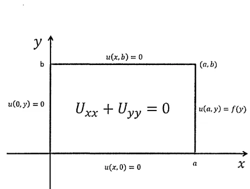
To solve the Dirichlet boundary value problem of Laplace’s equation in a rectan gular domain by separation of variables (see Figure 3.1) [Babuska, 1995; Gakhov, 1990; Haberman, 1983; Ritger and Rose, 1968; Wazwaz, 2002]:
where u(x,y) satisfies the non-homogeneous boundary condition, and / is a given
function.
By using the technique of separation of variables (a solution can be expressed as a product of unknown functions each of which depends only on one of the inde pendent variables), assume the solution to Laplace’s equation is separable form,
u(x,y) = X(x)Y(y). To compute the partial derivatives that we require within the equation, we note that
Uxx
+
U yy —0
where u(x,y) satisfies the homogeneous boundary conditions, and
(3.9)
w(0,y) = u{x,b) — u(x,0) = 0
u ( a ,y ) = f( y )
(3.10)
Uy{x,y) = ^{X{x)Y(y)) = X{x)Y'(y)
ux(x,y) = ^ (x (* )y (y )) = x '(x )y (y )
(3.11)
u(x, b) = 0
u(0,y) = 0 u(a,y) = f ( y )
[image:44.613.142.392.55.244.2]u(x, 0) = 0
Figure 3.1: Defining Laplace’s equation over a rectangular domain.
thus,
“yyfay) = ^ 2 (X W y W ) = ^ W y/,W
Uxx(x,y) = ^ ( X { x ) Y ( y ) ) = X"(x)Y(y)
(3.13)
(3.14)
Then Laplace’s equation 3.9 can be written as:
X"(x)Y(y)+X(x)Y"(y) = 0 (3.15)
That can be rearranged to form
X"(x) Y"(y)
X(x) Y{y) = X , (3.16)
where X is a separation constant. The left hand side depends only on while the
right hand side depends only on y. Thus Eqs.3.16 is partitioned into two ODEs as
X"(x) = XX(x), (3.17)
and
Let Y (y) satisfy the Dirichlet boundary condition
y(0) = Y(b) = 0. (3.19)
Eqs. 3.17 and 3.18 are ODE and can be solved with basic techniques. There
are three different cases, depending on the sign of X, each will give four different
solutions to Laplace’s equation. Then, solving for Y in Eq. 3.18 with the boundary
condition in Eq.3.19, the nontrivial solution is
K = c s i n ( ^ ) with X = (^ ) 2, (3.20)
v b ' b
where n = 1 ,2 , For the X in Eq.3.20, it is found that the general solution to
Eq. 3.17 is
X ( x ) = A e f x + B e - tT*. (3.21) or
n7L nTZ
X(x) = ci cosh [— l b (x — L)1 + J C2 sinh [— (* — L)1. b (3.22) The shift in x by L is selected to satisfy the boundary condition at x = L. It is
assumed thatX(L) = 0, which implies c\ = 0. Thus
yiTT
X(x) = C2sinh [— (x — L )]. (3.23)
Thus, it is found that the nontrivial product solutions to Laplace’s equation to gether with the homogeneous boundary conditions are constant multiples of
tVJZ
u(x,y) = C2sinh [— (* —L)] sm(nny/b). (3.24)
By the superposition principle theorem, we obtain
° ° M l
The coefficients cn are identified by the boundary condition
u(a,y) = Y i cn sin (nna/b) sinh(«7ty/&) = f(y). (3.26)
n= 1
Therefore the quantities cn sinh(nna/b) must be the coefficients in the Fourier sine
series of period 2b for / and are given by
An==l I o ^ Sin~b~^y' (3'27^
Thus, it can be written:
* - 5 h F ^ ] - <3-28)
Thus the solution to the partial differential Equation 3.9 satisfying the boundary
condition 3.10 as given by Eq 3.25 with the coefficients cn computed from Eq.
3.27. From Eqs.3.25 and 3.27 it can be seen that the solution contains the factor
sinh(mu:/&)/sinh(nna/b).
To estimate this quantity for large n one can use the approximation sinh^ = e^/2,
and thereby obtain
sinh(njw/fc) ^ \exp{nnx/b)
sinh(nna/b) ~ \ e x p [ ^ [ b ) ~ (3’29) Thus, this factor has the character of a negative exponential; consequently, the
series 3.25 converges quite rapidly unless a — A: is very small.
3.4.2 The solution by the method of lines
Therefore, another alternative method is to solve Laplace’s equation on a grid by the method of lines [Lord et al., 2014; Strang and Aarikka, 1986],
Uxx + Uyy = 0 (3.30)
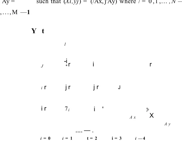
In Figure 3.2 divided the interval into N and M sub-intervals with Ax = ^ 1 ) ’
and Ay = such that (Xi,yj) = (/Ax, j'Ay) where / = 0 ,1 ,... ,N — 1, and j =
0,1,...,M — 1
Y t
1
-i . r
J *r i
i r j r j r j
'
i r 7i i
.... — .
"p A x X
A y
[image:47.614.101.401.182.422.2]i = 0 i = 1 t = 2 i = 3 i — 4
Figure 3.2: The value in green is given by the boundary condition, the only un
knowns are Utj marked in red.
The domain has four boundaries;
Ui,0 = g(Xi, 0), U w - i= g { x i, b ) / = 0, l,...,iV — 1 (3.31)
Uoj = g{0,yj), f /v - i j = 7—0,1,... ,M — 1.
The boundary conditions are simplified along the boundary (green), and the inte rior points (red) are unknowns.
Finite difference approximations must now be used to replace £/** and Uyy in the
Laplace’s equation. Focusing on an interior point (x/,yy), the simplest approxima tions to replace the second derivatives with it is a central finite difference approx imation as follow,
j, cv v \ ~ 17(* '-i ’>v) ~ 2 u (x‘>yj)+ u (x i+1 >yj) n
Uxx\Xhyj)~ (Ax)2 ’
and
* u{xhyj- ' ] - 2U^ J ) + u { x i'yj+l) (3.33)
Eqs 3.32 and 3.33 tend to be just like individuals for that regular second deriva
tives, d^u/dx2 and d2u/dy2, only that in Eqs. 3.32 y is held constant (all terms in
Eqs. 3.32 have the same j) and in Eqs. 3.33 x is held constant (all terms have the
same /). Eqs. 3.32 and 3.33 are equivalent to
u „ ( x ,y )« (Ax)z (3.34)
,, U ( x , y - A y ) - 2 U { x ,y ) + U(x,y + Ay)
Uyy\x ^y) ~ (Ay)2 IP
Connecting Eqs. 3.32 and 3.33 into the unique Laplace equation and by the used of the method of lines approximation, to obtain a system of ODEs
Ui—\,j~'ZUijJrUi+\j Uj j - \ — 2 /j + Uij+\
(Ae)2--- + ---( A ^ --- at the grid pointy,;).
(3.36) or
U i-ij + ty+ij — 4C//J + Uij-i + Uij+1 = 0 (3.37)
Assuming that Ax = Ay, where Uij = U (iAxJAy). That gives
y . . = Ui-l,l + Ui+lJ + UlJ-l + U‘J +1 (3-38)
Thus, Uij should be the average of its nearest neighbours. When the average
average have the potential to reach higher values after some iterations. Therefore,
when U reaches a highest on a few internal levels, then a similar highest can also
be achieved by each neighbour within this level. We can continue iterating this technique right up until we cover all the points in the rectangle, and we get the
vector U.
( Un ^
Vl2
Ui3
U = U2i , (3.39)
\ Umn
Moreover, Eq. 3.38 is an approximation of Laplace’s equation, and it is an M x N
matrix that can be solved as Jacobi iteration
(3.40)
where the superscript denote the iteration number and Uij is the solution at the i,j
grid point,
lim u } j +l) = UU . (3.41)
V->00 >4
Therefore, Uij is an excellent approximation to the exact solution to Laplace’s
equation.
3.5 Signal Representation
one-dimensional signals that can be represented by the following:
1. The Discrete Fourier Transform (DFT).
2. The Discrete Cosine Transform (DCT).
3. The Discrete Wavelet Transform (DWT).
4. The PDE-based Approach.
3.5.1 The Discrete Fourier Transform (DFT)
The discrete Fourier transform is a numerical approximation to the Fourier trans form, which is very useful in data compression, because a few coefficients of the Fourier expansion may be sufficient for the reconstructed signal to be close enough to the original function. It has already been found that the use of the FFT techniques has considerably enhanced the strength of digital techniques for a very wide range of problems such as spectral research, sign managing, graphic con trols, and also the solution of differential equations [Cooley et al., 1969; Hanna and Rowland, 2008]. The fast Fourier transform is an efficient algorithm for com puting the discrete Fourier transform DFT and its inverse, which takes a regularly spaced data value, then returns the value of the Fourier transform for a set of values in frequency space. Moreover, the FFT algorithm can decrease the pro cessing time of a standard Discrete Fourier Transform from several minutes to a few milliseconds, and it is global problem solving technique. The significance of Fourier Transform comes from allowing the evaluation of particular relationships in a problem domain from an entirely different viewpoint. Studying the behaviour of a function and its Fourier Transform is often the key to efficient problem solv ing [Weinberger, 2012].
defined as
/ M = £ [/(* ) ](v) (3.42)
f(t)e~ i2mdt. (3.43)
If the integral exists for each value of the parameter / then Eqs 3.43 defines /(v ), the Fourier Transform of /(/*)•
Now consider the generalisation to the situation of a discrete function, f ( t ) —> f(tic) by letting fa = f f a ) , where tk = kA , with k = 0 ,1 , — 1. Writing this
out gives the Discrete Fourier Transform Fn = fa {fa}^Q (n) as
F n = Z f k e ~ i2mk/N■ (3.44)
*=0
The inverse transform fa = (k) is then
fk = T, Z F»eiMn/N-
/V
(3'45>n
=0
Discrete Fourier Transforms are useful because they reveal periodicities in data views as well as the relative importance of regularity elements. There are a few details on the interpretation of Discrete Fourier Transforms, however. Typically, the Fourier Transform of an actual series will be a series of an actual and complex variant of the same duration. Particularly, if fa are real, then F^/-n and Fn are approximated by:
FN-n = Fn, (3.46)
for n = 0 ,1 ,..., N — 1, where z signifies the actual complex conjugate. Exactly
3.5.2 The Discrete Cosine Transform (DCT)
The Discrete Cosine Transform (DCT) are important to numerous types of lossy compression of audio and image, to solve PDE by spectral techniques where the different version of the DCT matches to slightly different even/odd border circum stances at the two ends of the range. The use of cosine rather than sine features is crucial in these applications: for compression, it can be seen that cosine functions are much more effective.
In particular, the DCT is equivalent to a DFT, but with only real values: the DCT is comparable to a DFT of approximately twice the length since the FFT of a real and even function is real and even, where in some versions the output is shifted by half a sample.
The most common DCT definition applied to 2D image compression is the fol lowing [Halpem et al., 2002]:
for m,v = 0 ,1 ,2 ,... , N — 1.
3.5.3 The Discrete Wavelet Transform (DWT)
The term ‘wavelet’ is used to describe a spatially localized function. ‘Localized’ means that the wavelet has compact support or it almost has compact support in the sense that outside some interval the amplitude of the wavelet decays expo nentially [Jameson, 1993]. Just like the Fourier sequence, wavelets are statistical features that are used to signify information or other features, by analysing the
n / \ / \ W r/ \ [7C(2*-F 1)k1
C(h,v) = cc(w)cx(v) £ £ / ( * , ? ) cos —
---;c=0 >’=0
for m, v = 0 ,1 ,2, . . . , N — 1. The inverse transform is defined as
2y + l ) v
N - l N - l
data according to scale. This function has developed mostly over the last 15 years and has generated tremendous interest in many areas of research in mathematics, physics, computer science, as well as architectural. However, most applications of wavelets have focused on analysing data and using wavelets as a tool for data compression.
Wavelet methods combine the advantages of both spectral (Fourier) and finite dif ference methods and allow both space and time dependent coefficients [Beylkin, 1993; Dahmen et al., 1999; Schneider and Vasilyev, 2009; Vasilyev and Kevlahan, 2005; Vasilyev et al., 1997; Xu and Shann, 1992]. Wavelets allow decomposition of a signal or an image into its components with respect to a whole cascade of levels. This decomposition is done by the fast wavelet transform (FWT) which is of linear complexity as long as the wavelet is compactly supported [Meyer,
1990]. Decomposition and reconstruction allow a signal or an image to be trans formed from one representation to a different one; namely, from a single scale to a multi-scale representation. However, successive application of these two opera tions, gives back the original signal or image as long as the corresponding filters are chosen appropriately. The reason why wavelets are so successful in signal and image processing lies in the fact that the multi-scale representation allows the modification of the signal or image for different purposes.
3.5.4 The PDE-based Approach
The PDE-based approach to global sensitivity analysis gives access to a profound theory and broad methodology. Methods of lines are generally simple to imple ment due to the possibility of using standard ODE solvers. Concerning error control, adaptive ODE solvers straightforwardly allow for temporal adaptivity. However, spatially adaptable methods of lines commonly rely on a posteriori er ror estimates, that require a complete solution of the system, before the spatial discretization can be adapted [see for instance [Adjerid et al., 1999]]. In that re spect, both methods offer a substantial advantage, since the temporal and spatial discretization can be adjusted in each integration step.
The method of lines is a technique that transforms a PDE into a set of ODEs with a single variable. The transformation is done by discretizing the PDE in space, leaving a number of unknowns and their time derivatives. For the space discretization, the techniques referred to previously may be used. For instance, when the finite difference technique can be used, the area discretization results in one unknown and its time derivative at each grid point in the domain, that is a set of ODEs. One advantage of the method of lines is that advanced numerical solution techniques can be found with regard to resolving common ODEs which not necessarily nevertheless are available regarding PDEs. There are, for instance, solvers with automatic step adjustment to find a solution with needed precision. An additional benefit is actually which combined techniques containing both ODE and PDE based models become much easier to solve since the space discretiza tion of the actual PDEs outcomes in ODEs that may be resolved with the already existing ODEs.
We-ickert, 2009; Peloquin, 2009; Sturmer et al., 2008] with promising results in 2D images that can be seen as single-value functions from pixel intensities. How ever, such methods have not attempted to encode arbitrary 3D geometries. Hence, the method of lines (MOL) given in Section 3.4.2 will be implemented in Sec tion 6.2.3.
3.6 Interpolation and Compression
Definition 3.6.1. Interpolation is the term used for methods that construct new data points from a discrete set of data points. Usually this means to construct a continuous function from a discrete set of function values.
Approximation (a curve fitting in ID) is similar to interpolation, but it does not necessarily pass through all data points. The advantage of this particular technique is that it frequently leads to a smoother reconstruction. The drawback is generally a reduction in accuracy, image resolution or maybe precision. Moreover, with
interpolation a function is sought that allows to approximate f( x) such that func
tional values between the original data set values may be determined. With the curve fitting, one simply requires a function that is a good fit to the original data points.
Definition 3.6.2. Compression is the process of encoding data by using as few information-bearing units (usually bits) as possible, such that the inverse process, called decoding, will return the original information [Pennebaker and Mitchell,
1993].
compressing a 3D object is to deal with geometry and connectivity (since prop erties can be dealt with in the same way as geometry) and a number of methods have been proposed since the early 1990s.
In general, there are three methods one can use to compress 3D data:
1. Image-based compression: where each snapshot of a 3D scene is com pressed as a 2D image. This is a palliative solution (for instance, flash animation of the three dimensional picture) and the shortcomings are that this is not fully interactive and not immersive.
2. Si