warwick.ac.uk/lib-publications
Original citation:
Pozzi, Paola and Stinner, Björn (2018) Elastic flow interacting with a lateral diffusion process
: the one-dimensional graph case. IMA Journal of Numerical Analysis.
doi:
10.1093/imanum/dry004
Permanent WRAP URL:
http://wrap.warwick.ac.uk/97333
Copyright and reuse:
The Warwick Research Archive Portal (WRAP) makes this work by researchers of the
University of Warwick available open access under the following conditions. Copyright ©
and all moral rights to the version of the paper presented here belong to the individual
author(s) and/or other copyright owners. To the extent reasonable and practicable the
material made available in WRAP has been checked for eligibility before being made
available.
Copies of full items can be used for personal research or study, educational, or not-for profit
purposes without prior permission or charge. Provided that the authors, title and full
bibliographic details are credited, a hyperlink and/or URL is given for the original metadata
page and the content is not changed in any way.
Publisher’s statement:
This is a pre-copyedited, author-produced PDF of an article accepted for publication in IMA
Journal of Numerical Analysis following peer review. The version of record Pozzi,
Paola and Stinner, Björn (2018) Elastic flow interacting with a lateral diffusion process : the
one-dimensional graph case. IMA Journal of Numerical Analysis.
is available online at
https://doi.org/10.1093/imanum/dry004
A note on versions:
The version presented here may differ from the published version or, version of record, if
you wish to cite this item you are advised to consult the publisher’s version. Please see the
‘permanent WRAP URL’ above for details on accessing the published version and note that
access may require a subscription.
arXiv:1707.08643v1 [math.NA] 26 Jul 2017
one-dimensional graph case
Paola Pozzi
∗Universit¨at Duisburg-Essen, Fakult¨at f¨
ur Mathematik,
Thea-Leymann-Straße 9, 45127 Essen, Germany
and
Bj¨
orn Stinner
†Mathematics Institute, University of Warwick,
Zeeman Building, Coventry CV4 7AL, United Kingdom
July 28, 2017
Abstract
A finite element approach to the elastic flow of a curve coupled with a diffusion equation on the curve is analysed. Considering the graph case, the problem is weakly formulated and approximated with continuous linear finite elements, which is enabled thanks to second-order operator splitting. The error analysis builds up on previous results for the elastic flow. To obtain an error estimate for the quantity on the curve a better control of the velocity is required. For this purpose, a penalty approach is employed and then combined with a generalised Gronwall lemma. Numerical simulations support the theoretical convergence results. Further numerical experiments indicate stability beyond the parameter regime with respect to the penalty term which is covered by the theory.
Keywords: geometric PDE, surface PDE, operator splitting, finite elements, convergence analysis
MSC 2010: 65M60, 35R01, 65M15
1
Introduction
The objective of this article is the convergence analysis of a semi-discrete finite element approximation to the following problem:
Problem 1.1. Given a spatial intervalI:= (0,1)and a time interval (0, T)with someT >0 and some functionsf :R→R,u0, c0:I→R, andub:∂I→R, find functions u, c:I×(0, T)→Rsuch that
ut
Q =− 1 Q
κx
Q
x
−12κ3+f(c), (1.1)
κ=
u
x
Q
x
, (1.2)
(cQ)t=
cx
Q
x
, (1.3)
∗Email: [email protected]
where
Q(x, t) :=p1 +u2
x(x, t), (x, t)∈I×(0, T),
with the boundary and initial conditions
u(x, t) =ub(x), κ(x, t) = 0, c(x, t) = 0, (x, t)∈∂I×[0, T], (1.4)
c(x,0) =c0(x), u(x,0) =u0(x), x∈I. (1.5)
The equations (1.1) and (1.2) are the graph formulation of the elastic flow for the curve{Γ(t)}t∈(0,T),
Γ(t) := {(x, u(x, t))|x∈I}, with a forcing termf(c) in the direction normal to the curve. This term depends on a conserved field c on the curve which is subject to the advection-diffusion equation (1.3). Such type of problems are motivated by applications in soft matter, see [24, 25, 32], and cell biology ([9, 34, 27]).
Numerical methods for solving forth-order geometric equations such as (1.1), (1.2) may be based on parametric approaches. This work builds up on the graph formulation of the elastic flow (or Willmore flow for higher dimensional manifolds) and on the results which are presented in [11, 10]. More general parametric methods for the above or related problems are presented and analysed in [23, 12, 3, 4] for curves and [1, 19, 38] for surfaces. Often, operator splitting is employed, thus enabling the use of H1
conforming spaces. But also more direct approaches exist, for instance, using finite volume techniques as in [33], employing methods from isogeometric analysis ([6]), or usingC1 conforming finite elements as in
[15, 14]. Alternatively, methods may also be based on interface capturing approaches. This includes level set representations of the curve or surface ([36, 16], see [7] for a comparison with parametric methods) and the phase field methodology ([17, 18, 8, 28]. For an overview we refer to [13] but we remark that the field has seen significant advances since.
The two paradigms of surface representation, parametric approaches versus interface capturing ap-proaches, also underpin techniques for solving PDEs on moving surfaces. The overview by [22] lists a variety of methods. These include Lagrange methods using finite elements on triangulated surfaces as in [20] or generalised spline representations, see [31], diffuse interface approximations ([40, 26]), or Eulerian approaches based on fixed bulk meshes ([41, 21, 35, 29, 37]).
For coupled problems such as (1.1)–(1.3) we are not aware of any convergence results. Schemes for curve shortening flow instead of the above elastic flow have been analysed in [39] (semi-discrete) and [2] (fully discrete). The related work of [30] covers the case of a (weighted) H1 flow instead anL2 flow of
the surface energy. The benefit then is some additional control of the manifold velocity which allows to show convergence of an isoparametric finite element scheme even in the case of surfaces.
Our numerical approach to Problem 1.1 is based on the method in [11, 10] for the elastic flow of the curve in the graph case. Operator splitting and piecewise linear H1-conforming finite elements are used
and, in particular, error estimates for the velocityut, the spatial gradientux, and the length element Q
are proved. However, the diffusion equation involvesQt, whence some control ofuxtis required. Denoting
byhthe spatial discretisation parameter, the idea is to add a suitablyh-weightedH1inner product of the velocity with the test function to the semi-discrete weak problem, see (3.6) and (3.8) below. In principle, this idea already features in the scheme in [39, equation (3.12)] where, thanks to mass lumping, such a term with a weighting scaling withh2is added. For that problem the structure of the geometric equation
could be further exploited in order to derive suitable error estimates for c. In the present case we use a generalised Gronwall inequality (see Lemma 4.9 below) instead. For this to work we need to assume strictly smaller than quadratic growth in h. As a result, we can only prove smaller convergence rates for the geometric fields than in [11]. The slower convergence is also observed in numerical simulations. However, the scheme turns out to be quite stable even for faster growth of the penalty term in h. In particular, if it grows quadratically inh then we essentially recover the rates in [11] (where there is no coupling, i.e.,f = 0).
of the semi-discrete scheme and state the main convergence result (Theorem 3.3 on page 6). This result then is proved by a series of Lemmas in Section 4. In Section 5 we present some numerical simulation results and Section 6 contains some concluding remarks.
2
Variational formulation and assumptions
Instead of working with the scalar curvatureκ, we introduce the variable
w:=−κQ=−κp1 +ux(x, t)2=−
uxx
(1 +ux(x, t)2).
A simple computation gives
−Q1
κ
x
Q
x
−12κ3=
1
Q3wx
x
+1 2
w2
Q3ux
x
.
We thus consider the following weak formulation of the system (1.1)–(1.3):
Z
I
ut
Qϕ dx+
Z
I
1 2w
2uxϕx
Q3 +
wxϕx
Q3 dx−
Z
I
f(c)ϕ dx = 0 ∀ϕ∈H01(I), (2.1)
Z
I
w Qψ dx−
Z
I
ux
Qψxdx = 0 ∀ψ∈H
1
0(I), (2.2)
d dt
Z
I
cQξ dx
+
Z
I
cx
Qξxdx = 0 ∀ξ∈H
1
0(I). (2.3)
Note that if we consider a time dependent test functionξthen the last equation is replaced by
d dt
Z
I
cQξ dx
+
Z
I
cx
Qξxdx=
Z
I
cQξt. (2.4)
Iff = 0 then the system (2.1), (2.2) coincides with [11, (2.4), (2.5)].
Assumption 2.1. We assume thatf :R→Ris a given continuously differentiable map with
kfkL∞(
R)≤C, kf′kL∞(
R)≤C. (2.5)
Moreover, we assume that the initial-boundary value problem (1.1)–(1.5) has a unique solution (u, c)
which satisfies
u∈L∞((0, T);W4,∞(I))∩L2((0, T);H5(I)), (2.6) ut∈L∞((0, T);W2,∞(I))∩L2((0, T);H3(I)), (2.7)
utt∈L∞((0, T);L∞(I))∩L2((0, T);H1(I)), (2.8)
c∈W1,∞((0, T);H1(I))∩L∞((0, T);H2(I))∩L∞((0, T);H1
0(I)). (2.9)
3
Discretisation and convergence statements
We consider continuous, piecewise linear finite elements on a subdivision 0 =x0< x1<· · ·< xN = 1 of
the spatial interval:
Letϕj, j = 0, . . . , N, denote the nodal basis functions. We set Xh:=span{ϕ0, . . . , ϕN} and denote by
Sj the subintervalSj= [xj−1, xj]⊂[0,1]. Moreover lethj =|Sj|andh= maxj=1,...,Nhjbe the maximal
diameter of a grid element. We assume that for some constant ¯C >0 we have
hj≥Ch¯ for allj= 1, . . . , N. (3.1)
For a continuous function u∈ C0([0,1],R) let I
hu ∈Xh be the linear interpolate uniquely defined by
Ihu(xi) =u(xi) for all i= 0, . . . , N. We shall use the standard interpolation estimates:
kv−IhvkL2(I)≤Chkkvk
Hk(I) fork= 1,2, (3.2)
k(v−Ihv)xkL2(I)≤ChkvkH2(I). (3.3)
Recall also the inverse estimates for anymh∈Xh andj= 1, . . . , N:
kmhxkL2(S j)≤
C hjk
mhkL2(S j)
(3.1)
=⇒ kmhxkL2(I)≤ C
hkmhkL2(I), (3.4)
kmhkL∞(S
j)≤
C
p
hjk
mhkL2(S j)
(3.1)
=⇒ kmhkL∞(I)≤ C
√
hkmhkL
2(I). (3.5)
The discrete formulation that we propose entails a regularization term weigthed by a positive function depending on the parameterh, which is defined by
µ(h) :=Cµhr for somer∈[1,2) and someCµ >0. (3.6)
The reason for introducing this term is motivated below in Remark 4.2 after introducing the necessary notation. The initial data for the discrete problem are denoted by
u0h∈Ih(ub) +Xh0, c0h∈Xh0, (3.7)
respectively, and will be specified in (4.23) below (see also Lemma 4.1).
Problem 3.1(Semi-discrete Scheme). Find functionsuh(·, t)∈Ih(ub) +Xh0andwh(·, t), ch(·, t)∈Xh0,
t∈[0, T], of the form
uh(x, t) = N
X
j=0
uj(t)ϕj(x), ch(x, t) = N−1
X
j=1
cj(t)ϕj(x), wh(x, t) = N−1
X
j=1
wj(t)ϕj(x),
with uj(t), cj(t), wj(t)∈ R, t ∈ [0, T], such that uh(·,0) =u0h, ch(·,0) =c0h as defined in (4.23), and
such that for all ϕh, ψh, ζh∈Xh0
Z
I
µ(h)uhxtϕhx+
uhtϕh
Qh dx+
Z
I
1 2w
2 h
uhxϕhx
Q3 h
+whxϕhx Q3
h
dx=
Z
I
Ih(f(ch))ϕhdx, (3.8)
Z
I
whψh
Qh
dx−
Z
I
uhxψhx
Qh
dx = 0, (3.9)
d dt
Z
I
chQhζhdx
+
Z
I
chxζhx
Qh
dx = 0. (3.10)
Here, µ(h)is defined in (3.6)andQh denotes the discrete length element,
Qh(x, t) :=
q
Note that if we consider a time dependent test functionζh(x, t) =PjN=1−1ζj(t)ϕj(x) in (3.10) then the
last equation is replaced by
d dt
Z
I
chQhζhdx
+
Z
I
chxζhx
Qh
dx =
Z
I
chζhtQhdx. (3.11)
Lemma 3.2. The above system (3.8)–(3.10)has a unique solution on [0,T˜] for any0<T <˜ ∞. Proof. Fix h > 0. Local existence on some time interval [0, Th) follows from standard ODEs theory.
Since uh(t), wh(t), ch(t) have values in a finite dimensional space (whose dimension depends onh), it is
sufficient to bound (uh, wh, ch) in some norm to obtain existence on [0,T˜]. Choosingϕh =uht in (3.8),
ψh =wh in (3.9)t (i.e. in equation (3.9) after differentiation with respect to time), and combining the
thus obtained equations gives
Z
I
µ(h)u2hxtdx+
u2 ht
Qh
dx+1 2 d dt Z I w2 h Qh dx= Z I
Ih(f(ch))uhtdx≤C
Z
I
Qhdx+
1 2 Z I u2 ht Qh ,
where for the last inequality we have used the boundedness off (recall (2.5)). Integration in time gives for anyt′
∈[0, Th)
µ(h)
Z t ′ 0 Z I u2
hxtdxdt+
1 2 Z t ′ 0 Z I u2 ht Qh
dxdt+1 2 Z I w2 h Qh
dx≤C(u0h, w0h) +C
Z t
′
0
Z
I
Qhdxdt.
On the other hand, using (3.9) we observe that
d dt
Z
I
Qhdx=
Z
I
wh
uht
Qh ≤ǫ
Z
I
u2 ht
Qhdx+Cǫ
Z
I
w2 h
Qhdx
so that integration in time gives
Z
I
Qh(t′)dx≤C(u0h) +ǫ
Z t′
0 Z I u2 ht Qh
dxdt+Cǫ
Z t′
0 Z I w2 h Qh
dxdt 0≤t′ < T
h.
Combining the above inequalities we obtain
µ(h)
Z t′
0
Z
I
u2hxtdxdt+
1 2
Z t′
0 Z I u2 ht Qh
dxdt+1 2 Z I w2 h Qh dx+ Z I
Qh(t′)dx
≤C+Cǫ
Z t′
0
Z
I
u2ht
Qh
dxdt+Cǫ
Z t′
0
Z
I
wh2
Qh
dxdt 0≤t′< Th,
for some constantC=C(u0h, w0h,T˜). Choosingǫappropriately and using a Gronwall argument we infer
that
µ(h)
Z t ′ 0 Z I u2
hxtdxdt+
Z t ′ 0 Z I u2 ht Qh dxdt+ Z I w2 h Qh
(t′)dx+Z
I
Qh(t′)dx≤C, 0≤t′< Th.
Since all norms are equivalent in a finite dimensional space, this implies thatQh(t′)≤C(u0h, w0h,T , h˜ )
uniformly in [0,1]×[0, Th). Uniform bounds foruh, wh follow immediately.
If we write down explicitly the ODE system for ˙uj then we see that
N−1
X
j=1
µ(h)
Z
I
ϕixϕjxdx+
Z
I
ϕiϕj
Qh dx
˙
with |Fi| ≤C uniformly in time, since f is bounded and since we have uniform bounds onwh and uh.
The (N−1)×(N−1) matrixAwith real entriesAij(h, Qh(t)) =RIµ(h)ϕixϕjx+ϕQiϕj
h dx is symmetric,
tri-diagonal, diagonalizable and positive definite. Its positive eigenvalues depend onhbut are uniformly bounded from below with repect to time (since Qh is uniformly bounded from above and below). For
simplicity we show this fact in the special case of a uniform grid and taking µ(h) =h(the general case is treated in a similar way): for the entries of the matrix A a simple computation gives (using that 1≤Qh(t′)≤C)
Aii =µ(h)
2 h+
Z
I
ϕ2 i
Qh(t′)
dx∈
2 + 1 C
4h 6 ,2 +
4h 6
,
Aii±1=−µ(h)1
h+
Z
I
ϕiϕi±1
Qh(t)
dx∈
−1 + 1 C
h 6,−1 +
h 6
.
It is well known (Gerschgorin theorem) that the eigenvaluesλ(t) ofA=A(t′) are elements of the set
{z∈R :|z−Aii| ≤ |Ai,i+1|+|Ai,i−1|}
giving that
5≥λ(t)≥ h
C, for 0≤t
′< T
h.
In conclusion we are able to infer a uniform bound on the ˙uj,j= 1, . . . , N−1 and hence onuhxt (taking
into account that ˙u0= ˙uN = 0 due to the boundary conditions).
Next, testing (3.11) withζh=ch and using the bounds onuh, uht we infer
d dt
Z
I
c2 hQhdx
+
Z
I
c2 hx
Qh
dx =
Z
I
chchtQhdx=
1 2
d dt
Z
I
c2 hQhdx
−1
2
Z
I
c2 h
uhx
Qh
uhxtdx
≤ 1
2 d dt
Z
I
c2hQhdx
+C
Z
I
c2hdx≤
1 2
d dt
Z
I
c2hQhdx
+C
Z
I
c2hQhdx.
With a Gronwall estimate we get kch(t′)kL2(I) ≤C = C(u0h, w0h,T , c˜ 0h, h) uniformly in 0 ≤t′ < Th.
The flow can be now extended up to time ˜T. Sincehwas chosen arbitrarily the claim follows.
We now state our main result which will be proved in the subsequent section by a series of lemmas:
Theorem 3.3. Let f :R→Rsatisfy (2.5). Assume that (1.1)–(1.5)has a unique solution(u, c)on the interval [0, T], which satisfies (2.6)–(2.9). Let (uh, ch)denote the solution of Problem 3.1. Then there is
someh0>0such that for all h≤h0
sup
0≤t≤Tk
(u−uh)(t)kL2(I)+ sup
0≤t≤Tk
(w−wh)(t)kL2(I)
+ sup
0≤t≤Tk
(u−uh)x(t)kL2(I)≤Ch,
Z T
0 k
(u−uh)t(t)k2L2(I)dt+
Z T
0 k
(w−wh)x(t)k2L2(I)dt≤Ch2,
sup
0≤t≤Tk
(c−ch)(t)k2L2(I)+
Z T
0 k
(c−ch)x(t)k2L2(I)dt≤Ch
2.
Moreover, we have that
Z T
0 k
(u−uh)tx(t)k2L2(I)dt≤C h2
µ(h) =Ch
2−r.
4
Error estimates
4.1
Nonlinear Ritz projections
Our error analysis relies strongly on results presented in [11], which are based on suitable nonlinear Ritz projections for u and w. We recall here their definition and properties. Let ˆuh be defined by:
ˆ
uh−Ih(ub)∈Xh0 and
Z
I
ˆ uhxξhx
ˆ Qh
=
Z
I
uxξhx
Q ∀ξh∈Xh0, (4.1)
ˆ
Qh(x, t) :=
q
1 + ˆu2 hx(x, t).
Note that timethere is a parameter only. For the error
ρu:=u−uˆh
we have the following estimates (see [11,§2] and references given in there; to simplify notation we write ρux for (ρu)x and so on):
sup
0≤t≤Tk
ρu(t)kL2(I)+h sup
0≤t≤Tk
ρux(t)kL2(I)≤Ch2, (4.2)
sup
0≤t≤Tk
ρu(t)kL∞
(I)+h sup 0≤t≤Tk
ρux(t)kL∞
(I)≤Ch2|logh|, (4.3)
sup
0≤t≤Tkρut(t)kL
2
(I)≤Ch2|logh|2, (4.4)
sup
0≤t≤Tk
ρutx(t)kL2(I)≤Ch. (4.5)
We also define a projection ˆwh∈Xh0ofw with the help of ˆuh as follows:
Z
I
E(ˆuhx) ˆwhxϕhxdx=
Z
I
E(ux)wxϕhxdx+
1 2
Z
I
w2 ux
Q3 −
ˆ uhx
ˆ Q3
h
!
ϕhxdx ∀ϕh∈Xh0 (4.6)
where we set
E(p) := 1 (1 +p2)3
2
forp∈R. (4.7)
Note that there is some constantC >0 such that|E(p)−E(q)| ≤C|p−q|for allp, q∈R. The proof of the following bounds for the error
ρw:=w−wˆh
is given in [11, Appendix, Lemma A.1]:
sup
0≤t≤Tk
ρwx(t)kL2
(I)≤Ch, (4.8)
sup
0≤t≤Tk
ρw(t)kL2(I)≤Ch2|logh|, (4.9)
sup
0≤t≤Tk
ρwtx(t)kL2(I)≤Ch, (4.10)
sup
0≤t≤Tk
The equations (2.6), (2.7), (4.3)–(4.5), (4.8)–(4.11) together with interpolation and inverse estimates imply that
kuˆhkW1,∞(I),kuˆhtkW1,∞(I),kwˆhkW1,∞(I),kwˆhtkW1,∞(I)≤C (4.12) uniformly inhand time.
4.2
Discrete initial data and first estimates
Let (uh, wh, ch) be the discrete solution on the time interval [0, T]. Define
C0:= sup x∈I, t∈[0,T]
Q(x, t), C1:= sup
x∈[0,1], t∈[0,T]|
w(x, t)|, (4.13)
C2:=kckC([0,T],H1(I)), C3:=kckL2((0,T),H1(I)). (4.14)
For the discrete solution we observe that on the time interval [0,¯t] (for ¯tsufficiently small) we have that
sup
x∈I, t∈[0,¯t]
Qh(x, t)≤2C0, sup
x∈I, t∈[0,¯t]|
wh(x, t)| ≤2C1, (4.15)
kchkC([0,¯t],L∞
(I))≤2 ˆC(I)C2, kchkL2((0,¯t),H1(I))≤2C3 (4.16)
thanks to the choice of initial conditions (see Lemma 4.1 below), the smoothness assumptions on (u, c), and a continuity argument (here, ˆC(I) denotes the constant for the embedding H1(I)֒→L∞(I) which
depends on the length ofI; in our caseI= (0,1) one can actually bound ˆC(I) by one). Define
Th:= sup{¯t∈[0, T]|(4.15),(4.16) hold on [0,¯t]}. (4.17)
We employ the well known strategy to first derive error estimates on the time interval [0, Th) and then
use these bounds to infer that Th = T. Therefore in what follows we shall assume (4.15) and (4.16)
(without specifying this in every statement). We decompose the errorsu−uh andw−whaccording to
u−uh= (u−uˆh) + (ˆuh−uh) =ρu+eu, whereeu:= ˆuh−uh,
w−wh= (w−wˆh) + ( ˆwh−wh) =ρw+ew, whereew:= ˆwh−wh.
Sometimes it is convenient to work with the smooth and discrete unit normals
ν= (−ux,1)
Q , νˆh:=
(−uˆhx,1)
ˆ Qh
, νh:=
(−uhx,1)
Qh
.
Note that in [11, (3.4)] it is shown that
|νˆh−νh| ≤ |(ˆuh−uh)x| ≤(1 + sup I |
ˆ
uhx|)Qh|νˆh−νh|, (4.18)
which leads to
|νˆh−νh| ≤ |(ˆuh−uh)x|=|eux| ≤C|νˆh−νh|, (4.19)
where the constantC depends onC0 and on the constant appearing in (4.12). Clearly
|Qˆh−Qh| ≤
|(ˆuhx,−1)| − |(uhx,−1)|
≤
(ˆuhx,−1)−(uhx,−1)
=|uˆhx−uhx|=|eux|. (4.20)
In the estimates that will follow we will also use the fact that
|Q−Qh| ≤ |ux−uhx| ≤ |ρux|+|eux|, (4.21)
|ν−νh|=
(Qh−Q)
Qh
1
Q(ux,−1) + 1 Qh
(ux−uhx,0)
≤
which easily follow employing the boundedness ofQandQh.
We pick the following initial values in (3.7):
u0h(x) := ˆu0(x), c0h(x) :=Ih(c0)(x), x∈I,¯ (4.23)
where ˆu0 is the non-linear projection ofu0defined in (4.1).
Lemma 4.1. For the choice of initial data in (4.23) we have that
eu(0)≡0, kew(0)kL2(I)≤Ch.
Proof. The first statement follows directly from the definition. For the error estimate ofew(0), observe
that since ˆuh(·,0) =u0h(·) then by (3.9), (4.1), and (2.2)
Z
I
wh(0)ξh
Qh(0) =
Z
I
u0hxξhx
Qh(0) =
Z
I
u0xξhx
Q(0) =
Z
I
w(0)ξh
Q(0)
for anyξh∈Xh0. Subtraction gives
Z
I
w(0)
Q(0)− wh(0)
Qh(0)
ξh= 0 ∀ξh∈Xh0.
Testing withξh=Ih(w(0))−wh(0) gives
Z
I
|w(0)−wh(0)|2
Qh(0) =
Z
I
w(0)(w(0)−wh(0))Q(0)−Qh(0)
Q(0)Qh(0)
+
Z
I
(w(0)−wh(0))
Qh(0)
(w(0)−Ih(w(0)))
+
Z
I
w(0) Q(0)Qh(0)
(Qh(0)−Q(0))(w(0)−Ih(w(0))).
We infer thatkw(0)−wh(0)kL2(I)≤Chby a standardǫ-Young argument, (4.2), (2.6), (3.2), (4.12), and
the boundedness of 1≤Qh(0)≤C0+CkρuxkL∞ ≤3
2C0by (4.3), (4.12), andhsmall enough. The claim
now follows by writingew(0) =−ρw(0) + (w(0)−wh(0)) and using (4.9).
Remark 4.2. In the discrete formulation of the problem we have introduced a regularization term weigthed by µ(h). This is motivated by the necessity of finding an error estimate for |(Q−Qh)t| in Lemma 4.8
below (cf. term K1 in the proof ). Note that we can write
|(Q−Qh)t|=
uhx
Qh
(uxt−uhxt) +uxt(ux
Q − uhx
Qh
)
≤ |
ρuxt|+|euxt|+C|ν−νh|.
The regularisation helps in deriving an estimate for the “tricky” term |euxt|, see (4.37) below.
4.3
Error estimates for
e
uand
e
wThe following error estimates for eu and ew are obtained through appropriate modification of the
Lemma 4.3. Suppose that F :R→Ris twice continuously differentiable and thatζ∈H1
0(I). Then
Z
I
(F(ux)−F(ˆuhx))ζ dx=
Z
I
ρu ∂
∂x(ζF
′
(ux))dx+R,
where Rsatisfies|R| ≤Ch2|logh|kζk L2(I).
Proof. See [11, Lemma 3.1]. It uses a mean value theorem, the smoothness ofF andu(recall (2.6)) and the bounds (4.2), (4.3), and (4.12).
Lemma 4.4. For every ǫ >0 there existsCǫ such that
keux(t)k2L2(I)≤ǫkew(t)k2L2(I)+Cǫkeu(t)k2L2(I)+Ch4|logh|2, 0≤t < Th.
Proof. See [11, Lemma 3.2]. Here one starts from the equation
Z I uˆ hx ˆ Qh
−uQhx
h
ϕhxdx=
Z I w Q− wh Qh
ϕhdx ∀ϕ∈Xh0,
which follows from (4.1), (2.2), and (3.9), and tests withϕh=eu.
Lemma 4.5. For 0≤t < Th we have
kewx(t)k2L2(I)≤C(keux(t)k
2
L2(I)+keut(t)k
2
L2(I)+kew(t)k
2
L2(I)+h
4
|logh|4)
+Ck(c−ch)(t)k2L2(I)+Cµ(h)2kuhxt(t)k2L2(I)+Ch2(1 +kchx(t)k2L2(I)).
Proof. The definition (4.6) of ˆwhand (2.1) yield
Z
I
ˆ uhtϕh
Qh
+
Z
I
E(ˆuh) ˆwhxϕhx+
1 2 Z I ˆ w2 h ˆ Q3 h ˆ uhxϕhx
=
Z
I
(ˆuht−ut)ϕh
Qh + Z I ut 1
Qh −
1 Q
ϕh+
1 2
Z
I
( ˆwh2−w2)
ˆ uhx
ˆ Q3
h
ϕhx+
Z
I
f(c)ϕh
for allϕh∈Xh0. Subtracting (3.8) we obtain
Z
I
eutϕh
Qh +
Z
I
(E(ˆuhx) ˆwhx−E(uhx)whx)ϕhx+
1 2 ˆ w2 h ˆ Q3 h ˆ uhx−
w2 h Q3 h uhx !
ϕhx (4.24)
=−
Z
I
ρutϕh
Qh + Z I ut 1 Qh −
1 Q
ϕh+1
2
Z
I
( ˆw2h−w2)
ˆ uhx ˆ Q3 h ϕhx + Z I
(f(c)−Ih(f(ch)))ϕh+µ(h)
Z
I
uhxtϕhx.
After insertingϕh=ew∈Xh0we derive
Z
I
(E(ˆuhx) ˆwhx−E(uhx)whx)ewx=−
Z
I
eutew
Qh −
1 2 ˆ w2 h ˆ Q3 h ˆ uhx−
w2 h Q3 h uhx !
ewx−
Z
I
ρutew
Qh (4.25) + Z I ut 1 Qh−
1 Q
ew+1
2
Z
I
( ˆwh2−w2)
ˆ uhx ˆ Q3 h ewx + Z I
(f(c)−Ih(f(ch)))ew+µ(h)
Z
I
For the last two terms we observe that
µ(h)
Z
I
uhxtewx
≤ǫkewxk
2
L2(I)+Cǫµ(h)2kuhtxk2L2(I),
and Z I
(f(c)−Ih(f(ch)))ew
≤ Z I
(f(c)−f(ch))ew
+ Z I
(f(ch)−Ih(f(ch)))ew
≤Ckc−chkL22(I)+Ch2(1 +
Z
I|
chx|2) +Ckewk2L2(I) (4.26)
where we have used (2.5) and (3.2). From now on we argue exactly as in [11, Lemma 3.3]. The error bound relies on the fact that it can be shown that
Z
I
(E(ˆuhx) ˆwhx−E(uhx)whx)ewx≥ 1
2p
1 + 4C2 0
kewxk2L2(I)−Ckeuxk2L2(I).
The estimates for the remaining terms on the right-handside of (4.25) are carefully explained in [11, Lemma 3.3], hence we do not repeat the arguments here.
Lemma 4.6. For 0≤t < Th we have
µ(h) 2 keutxk
2 L2(I)+
1 4C0k
eutk2L2(I)+
Z
I
(E(ˆuhx) ˆwhx−E(uhx)whx)eutx+
1 2 Z I ˆ w2 h ˆ Q3 h ˆ uhx−
w2 h Q3 h uhx ! eutx
≤ −dtd
Z
I
utux
Q3euxρu+
1 2 d dt Z I
( ˆw2h−w2)
ˆ uhx
ˆ Q3
h
eux+Ckeuxk2L2(I)+Ch4|logh|4
+Ckc−chk2L2(I)+Cµ(h)2+Cµ(h)h2+Ch2(1 +kchxk2L2(I)).
Proof. Choosingϕ=eut∈Xh0 in (4.24) and using (4.15) we obtain
Z
I
e2 ut
2C0
+
Z
I
(E(ˆuhx) ˆwhx−E(uhx)whx)eutx+
1 2 ˆ w2 h ˆ Q3 h ˆ uhx−
w2 h Q3 h uhx ! eutx ≤ − Z I
ρuteut
Qh + Z I ut 1
Qh −
1 ˆ Qh
eut+
Z I ut 1 ˆ Qh − 1 Q
eut+
1 2
Z
I
( ˆw2 h−w2)
ˆ uhx ˆ Q3 h ϕhx + Z I
(f(c)−Ih(f(ch)))eut+µ(h)
Z
I
uhxteutx=:I+II+III+IV +V +V I.
The termsI, II, III, IV are treated and estimated as in [11, Lemma 3.4]. Again we refrain from giving details here since the original paper gives all argument in detail. For the fifth term we proceed as in (4.26) but with an ǫweight and obtain that
Z I
(f(c)−Ih(f(ch)))eut
≤
Cǫkc−chk2L2
(I)+ 2ǫkeutk2L2
(I)+Cǫh2(1 +
Z
I|
chx|2).
For the last term we compute using integration by parts (recall that eut= 0 on∂I)
V I =µ(h)
Z
I
uhtxeutx=µ(h)
Z
I
(uhtx−uˆhtx)eutx+
Z
I
(ˆuhtx−utx)eutx+
Z
I
utxeutx
=−µ(h)keutxk2L2(I)−µ(h)
Z
I
ρutxeutx−µ(h)
Z
I
utxxeut
≤ −µ(h)keutxk2L2(I)+ µ(h)
2 keutxk
2 L2(I)+
µ(h) 2 Ch
2+ǫke
where we have used (4.5) and (2.7). An appropriate choice ofǫtogether with the estimates for the terms I–V Igives the claim.
Lemma 4.7. For 0≤t < Th we have
1 2 d dt Z I e2 w
Qh −
1 2 Z I e2 w Q2 h
Qht−
Z I ˆ wh ˆ Qht ˆ Q2 h
−QQht2 h
!
ew−
Z
I
(E(ˆuhx)ˆuhtx−E(uhx)uhtx)ewx
≤ǫkewxk2L2(I)+Cǫ(keuxk2L2(I)+kewk2L2(I)) +Cǫh4|logh|4.
Proof. See [11, Lemma 3.5]: the main idea is to take equation (2.2) together with the definition of ˆuh
(recall (4.1)) to infer
Z I wξh Q = Z I
uxξhx
Q =
Z
I
ˆ uhxξhx
ˆ Qh
∀ξh∈Xh0,
and from which differentiation with respect to time gives
Z
I
wtξh
Q −
Z
I
wξh
Q2 Qt−
Z
I
E(ˆuhx)ˆuhtxξhx= 0 ∀ξh∈Xh0. (4.27)
Differentiation with respect to time of (3.9) gives
Z
I
whtξh
Qh −
Z
I
whξh
Q2 h
Qht−
Z
I
E(uhx)uhtxξhx= 0 ∀ξh∈Xh0. (4.28)
The claim now follows by taking the difference of (4.27), (4.28), and testing withξh=ew.
It follows now from Lemma 4.6 and Lemma 4.7 that
µ(h) 2 keutxk
2 L2(I)+
1 4C0k
eutk2L2(I)+
1 2 d dt Z I e2 w Qh +1 2 Z I ˆ w2 h ˆ Q3 h ˆ uhx− w
2 h Q3 h uhx !
eutx−1
2 Z I e2 w Q2 h
Qht−
Z I ˆ wh ˆ Qht ˆ Q2 h
−QQht2 h ! ew + Z I
(E(ˆuhx) ˆwhx−E(uhx)whx)eutx−
Z
I
(E(ˆuhx)ˆuhtx−E(uhx)uhtx)ewx
≤ −dtd
Z
I
utux
Q3euxρu+
1 2 d dt Z I
( ˆw2h−w2)
ˆ uhx
ˆ Q3
h
eux+Cǫh4|logh|4
+ǫkewxk2L2(I)+Cǫ(keuxk2L2(I)+kewk2L2(I))
+Ckc−chk2L2(I)+Cµ(h)2+Cµ(h)h2+Ch2(1 +kchxk2L2(I)). (4.29)
The terms appearing is the second and third line are dealt with as in [11, p34–37] where the lengthy calculations are presented in detail. We thus only list the relevant results. Precisely one finds that (see [11, (3.15), (3.18), (3.19)])
1 2 Z I ˆ w2 h ˆ Q3 h ˆ uhx−
w2 h Q3 h uhx !
eutx−
1 2 Z I e2 w Q2 h
Qht−
Z I ˆ wh ˆ Qht ˆ Q2 h
−Qht
Q2 h
!
ew (4.30)
≥12dtd
Z
I
ˆ w2h
( 1 2 Qh ˆ Q2 h
|νˆh−νh|2−
1 QhQˆ2h
( ˆQh−Qh)2
)
−C(kewk2L2
(I)+keuxk2L2
as well as
Z
I
(E(ˆuhx)−E(uhx))(ˆuhtx−uhtx) ˆwhx (4.31)
≥ d
dt
Z
I
Q
h
ˆ Qh
−1
(ˆνh−νh)−
1 2
Qh
ˆ Qh
|νˆh−νh|2νˆh
·( ˆwhx,0)t−Ckeuxk2L2(I),
and
Z
I
(E(ˆuhx)−E(uhx))ˆuhtxewx
≤
ǫkewxk2L2(I)+Cǫkeuxk2L2(I). (4.32)
Observing that
(E(ˆuhx) ˆwhx−E(uhx)whx)eutx−(E(ˆuhx)ˆuhtx−E(uhx)uhtx)ewx
= (E(ˆuhx)−E(uhx))(ˆuhtx−uhtx) ˆwhx−(E(ˆuhx)−E(uhx))ˆuhtxewx,
and inserting (4.30), (4.31), (4.32) into (4.29) we obtain
µ(h) 2 keutxk
2 L2(I)+
1 4C0k
eutk2L2(I)+
1 2
d dt
Z
I
e2 w
Qh
≤ −dtd
Z
I
ut
ux
Q3euxρu+
1 2
d dt
Z
I
( ˆw2h−w2)
ˆ uhx
ˆ Q3
h
eux
−12dtd
Z
I
ˆ wh2
(
1 2
Qh
ˆ Q2
h
|νˆh−νh|2− 1
QhQˆ2h
( ˆQh−Qh)2
)
−dtd
Z
I
Q
h
ˆ Qh
−1
(ˆνh−νh)−1
2 Qh
ˆ Qh
|νˆh−νh|2νˆh
·( ˆwhx,0)t
+Cǫh4|logh|4+ǫkewxk2L2(I)+Cǫ(keuxk2L2(I)+kewk2L2(I))
+Ckc−chk2L2(I)+Cµ(h)2+Cµ(h)h2+Ch2(1 +kchxk2L2(I)).
Integration with respect to time for some ¯t ∈(0, Th), application of Lemma 4.4 and Lemma 4.5, (4.12),
(4.19), (4.15), (4.16), (4.2), and using the approximation order of the initial data (recall Lemma 4.1) yields
Z ¯t
0
µ(h)keutxk2L2(I)dt+
Z ¯t
0 k
eutk2L2(I)dt+kew(¯t)k2L2(I)
≤Ckew(0)k2L2(I)+Ckeux(¯t)kL2(I)(kρu(¯t)kL2(I)+kew(¯t)kL2(I)+keux(¯t)kL2(I))
+Ckeux(0)kL2(I)(kρu(0)kL2(I)+kew(0)kL2(I)+keux(0)kL2(I))
+Cǫh4|logh|4+ǫ
Z ¯t
0 k
ewxk2L2(I)dt
+Cǫ
Z ¯t
0
(keuxk2L2(I)+kewk2L2(I))dt+C
Z t¯
0 k
c−chk2L2(I)dt
+Cµ(h)2+Cµ(h)h2+Ch2(1 +
Z ¯t
0 k
chxk2L2(I)dt)
≤ǫ kew(¯t)k2L2(I)+
Z t¯
0 k
eutk2L2(I)dt
!
+ǫCµ(h)2
Z ¯t
0 k
+Cǫ keu(¯t)k2L2(I)+h4|logh|4+
Z ¯t
0
(keuk2L2(I)+kewk2L2(I))dt
!
+C
Z t¯
0 k
c−chk2L2
(I)dt+Cµ(h)
2+Cµ(h)h2+Ch2. (4.33)
Thanks to (4.12) and asµ(h)≤1 for allh≤h0 with some sufficiently smallh0we have that
ǫCµ(h)2
Z t¯
0 k
uhxtk2L2(I)dt
≤ǫCµ(h)2
Z t¯
0
(keutxk2L2
(I)+C)dt≤ǫCµ(h)
Z ¯t
0 k
eutxk2L2
(I)dt+ǫCµ(h)
2. (4.34)
Moreover, using that eu(0) = 0 we obtain that
keu(¯t)k2L2(I)=
Z ¯t
0
d dt
eu(t)
2
L2(I)dt=
Z ¯t
0
Z
I
2eueutdxdt≤ǫ
Z ¯t
0 k
eutk2L2(I)dt+Cǫ
Z ¯t
0 k
euk2L2(I)dt.
Using this and (4.34) with ǫsmall enough in (4.33) yields
Z ¯t
0
µ(h)keutxk2L2(I)dt+
Z ¯t
0 k
eutk2L2(I)dt+kew(¯t)k
2
L2(I)+keu(¯t)k
2 L2(I)
≤C
Z ¯t
0
(keuk2L2(I)+kewk2L2(I))dt+C
Z t¯
0 k
c−chk2L2(I)dt+Cµ(h)2+Cµ(h)h2+Ch2. (4.35)
A Gronwall argument and using that µ(h) ≤ Ch for all h ≤h0 (after eventually reducing h0) finally
yields
kew(¯t)k2L2(I)+keu(¯t)k2L2(I)≤C
Z t¯
0 k
c−chk2L2(I)dt+Ch2, ¯t∈[0, Th), (4.36)
from which also conclude that
µ(h)
Z ¯t
0 k
eutxk2L2(I)dt+
Z t¯
0 k
eutk2L2(I)dt≤C
Z ¯t
0 k
c−chk2L2(I)dt+Ch2, ¯t∈[0, Th). (4.37)
4.4
Error estimate for
(
c
−
c
h)
In order to proceed we need to analyse the error betweenc andch. We here basically follow the lines of
[39], Lemma 4.2. But we need to provide all details as the treatment of the terms with the time derivative of the length element is different here.
Lemma 4.8. We have that for any ¯t∈[0, Th)
kc(¯t)−ch(¯t)k2L2(I)+
Z ¯t
0 k
cx−chxk2L2(I)dt
≤Ckeux(¯t)k2L2(I)+C
Z ¯t
0 k
c−chk2L2(I)dt+C
Z ¯t
0 k
euxk2L2(I)dt+C
Z t¯
0 k
eutk2L2(I)dt
+C
Z t¯
0 k
euxk2L2(I)keutxk2L2(I)dt+Ch2
Z ¯t
0 k
Proof. The difference between the continuous (2.4) and the discrete version (3.11) reads
Z
I
(cQ−chQh)tζhdx+
Z
I
cx
Q − chx
Qh
ζhxdx= 0
for all test functionsζh(x, t) of the formζh=PN
−1
j=1 ζj(t)ϕj(x). Choosing
ζh=Ih(c)−ch=c−ch+Ih(c)−c
a calculation (cf. [39, Lemma 4.2]) yields that
d dt
Z
I
1
2(c−ch)
2Q hdx
+
Z
I
|(c−ch)x|2
Qh
dx
=
Z
I
c(Qh−Q)t(c−ch)dx−
Z
I
1
2(c−ch)
2Q htdx
+ d dt
Z
I
(cQ−chQh)(c−Ih(c))dx
−
Z
I
(cQ−chQh) c−Ih(c)tdx
+
Z
I
(c−ch)x(c−Ih(c))x
Qh
dx
+
Z
I
cx(c√−ch)x
Qh
Q−Qh
√
QhQ
dx+
Z
I
cx(Ih(c)−c)xQ−Qh
QhQ
dx
=
7
X
j=1
Kj. (4.38)
For the first term we can write
−K1=
Z
I
ct(Q−Qh)(c−ch)dx+
Z
I
c(Q−Qˆh)t(c−ch)dx+
Z
I
c( ˆQh−Qh)t(c−ch)dx
=:K1,0+K1,1+K1,2.
Using (4.21), the smoothness assumptions onc(recall (2.9)) and (4.2) we infer immediately that
|K1,0| ≤Ckc−chkL2
(I)(kρuxkL2
(I)+keuxkL2
(I))≤Ckc−chk2L2(I)+Ckeuxk2L2(I)+Ch2.
Next we write using (4.5), (4.12), the fact that|ν−νˆh| ≤C|ρux|and (4.2)
|K1,1|=
Z
I
c(Q−Qˆh)t(c−ch)
=
Z
I
c(c−ch)(ux
Q − ˆ uhx
ˆ Qh
)ˆuhtx+
Z
I
c(c−ch)ux
Q(utx−uˆhtx)
≤Ckc−chkL2(I)kν−νˆhkL2(I)+Ckc−chkL2(I)kρutxkL2(I)
≤Chkc−chkL2(I)≤Ckc−chk2
L2(I)+Ch
For the last term we observe using partial integration that
K1,2=
Z
I
c( ˆQh−Qh)t(c−ch) =
Z
I
c(c−ch)
uˆ
hx
ˆ Qh
ˆ uhtx−
uhx Qh uhtx = Z I
c(c−ch)ˆuhtx
uˆ
hx
ˆ Qh
−uhx
Qh
+
Z
I
c(c−ch)
u
hx
Qh −
ux
Q
(ˆuhtx−uhtx)
+
Z
I
c(c−ch)
ux
Q(ˆuhtx−uhtx) =
Z
I
c(c−ch)ˆuhtx
uˆ
hx
ˆ Qh
−uhx
Qh
+
Z
I
c(c−ch)
u
hx
Qh −
ux
Q
(ˆuhtx−uhtx)
− Z I ∂ ∂x
c(c−ch)
ux
Q
(ˆuht−uht).
Therefore we infer using (4.12), (4.19), (4.22), (4.2), and embedding theory that
|K1,2| ≤Ckc−chkL2(I)keuxkL2(I)+CkeutkL2(I)(kc−chkL2(I)+k(c−ch)xkL2(I))
+Ckc−chkL∞
(I)kν−νhkL2(I)keutxkL2(I)
≤Ckc−chk2L2(I)+Ckeuxk2L2(I)+ǫk(c−ch)xk2L2(I)+Cǫkeutk2L2(I)
+Ckc−chkH1(I)(h+keuxkL2(I))keutxkL2(I)
≤Ckc−chk2L2(I)+Ckeuxk2L2(I)+ǫk(c−ch)xk2L2(I)+Cǫkeutk2L2(I)
+Cǫkeuxk2L2(I)keutxk2L2(I)+Cǫh2keutxk2L2(I).
Putting all previous estimate together we infer that
|K1| ≤Ckc−chk2L2(I)+Ckeuxk2L2(I)+ǫk(c−ch)xk2L2(I) (4.39)
+Cǫkeutk2L2(I)+Cǫkeuxk2L2(I)keutxk2L2(I)+Cǫh2keutxk2L2(I)+Ch2.
The term K2 can be estimated as follows using integration by parts, the fact that kc−chkL∞ is bounded (thanks to (4.16)), (4.12), and (4.4):
|K2|=
1 2 Z I
(c−ch)2Qht
≤ 1 2 Z I
(c−ch)2Qt
+ 1 2 Z I
(c−ch)2(Qht−Qt)
≤Ckc−chk2L2(I)+
1 2 Z I
(c−ch)2
h
(uhx Qh −
ux
Q)uhtx+ ux
Q(uhtx−utx)
i
≤Ckc−chk2L2
(I)+kc−chkL∞(I)
1 2 Z I
(c−ch)(
uhx
Qh −
ux
Q)(uhtx−uˆhtx)
+kc−chkL∞(I)
1 2 Z I
(c−ch)(
uhx
Qh −
ux
Q)ˆuhtx
+ 1 2 Z I ∂ ∂x
(c−ch)2
ux
Q
(uht−ut)
≤Ckc−chk2L2(I)+Ckc−chkL∞(I)kνh−νkL2(I)keutxkL2(I)+Ckνh−νk2
L2(I)
+ǫk(c−ch)xk2L2(I)+Cǫkeutk2L2(I)+Cǫh4|logh|4.
The second term in the last line of above inequality can be treated as the same term appearing in K1,2,
so that we obtain
|K2| ≤Ckc−chk2L2(I)+Ckeuxk2L2(I)+ǫk(c−ch)xk2L2(I) (4.40)
+Cǫkeutk2L2
(I)+Cǫkeuxk2L2
(I)keutxk2L2
(I)+Cǫh2keutxk2L2
The remaining termsK3, . . . , K7are estimated as in [39, Lemma 4.2]. Precisely: ForK3we note that
by (2.9), (4.15), (3.2), (4.21), and (4.2)
Z
I
(cQ−chQh)(c−Ih(c))dx
= Z
I
(c−ch)Qh(c−Ih(c))dx+
Z
I
c(Q−Qh)(c−Ih(c))dx
≤εˆ
Z
I
(c−ch)2Qhdx+C
Z
I
(Q−Qh)2dx+Cεˆh4kck2H2(I)
≤εˆ
Z
I
(c−ch)2Qhdx+Ckeuxk2L2(I)+Cεˆh2 (4.41)
with ˆε >0 that will be picked later on. We will refer to this estimate later on when integrating (4.38) with respect to time.
For the termK4we infer from (3.2), (4.15), (2.9), (4.21), and (4.2), that
|K4|=
Z
I
c(Q−Qh)(ct−Ih(ct))dx+
Z
I
(c−ch)(ct−Ih(ct))Qhdx
≤C
Z
I
(Q−Qh)2dx+C
Z
I
(c−ch)2Qhdx+Ckctk2H1(I)h2
≤Ckc−chk2L2(I)+Ckeuxk2L2(I)+Ch2.
By the interpolation estimates (3.2), (3.3), embedding theory, (2.9), (4.21), and (4.2) we have the following estimates for the terms involving spatial gradients (forǫ >0 arbitrarily small):
|K5| ≤ǫ
Z
I
|(c−ch)x|2
Qh
dx+Cǫ
Z
I
|(c−Ih(c))x|2
Qh
dx
≤ǫ
Z
I
|(c−ch)x|2
Qh
dx+Cǫkck2H2
(I)h 2,
|K6| ≤ǫ
Z
I
|(c−ch)x|2
Qh
dx+Cǫkeuxk2L2
(I)+Cǫh2,
|K7| ≤Ckck2H2(I)h2+Ckeuxk2L2(I)+Ch2.
Summarizing all these estimates and using (4.15) we obtain from (4.38) that
d dt
Z
I
1 2|c−ch|
2
|Qh|dx
+
Z
I
|cx−chx|2
Qh
dx
≤ǫC
Z
I
|cx−chx|2
Qh
dx
+ d dt
Z
I
(c−ch)Qh(c−Ih(c))dx+
Z
I
c(Q−Qh)(c−Ih(c))dx
+C
Z
I|
c−ch|2Qhdx+CǫkeuxkL22(I)+Cǫkeutk2L2(I)
+Cǫkeuxk2L2(I)keutxk2L2(I)+Cǫh2keutxkL22(I)+Cǫh2.
enough that
Z
I|
c(¯t)−ch(¯t)|2dx+
Z ¯t
0
Z
I|
cx−chx|2dxdt
≤C
Z
I|
c0−c0h|2dx+
Z
I|
(c0Q(0)−c0hQh(0))(c0−Ih(c0))|dx
+Cεˆ
Z
I|
c(¯t)−ch(¯t)|2dx+Ckeux(¯t)k2L2(I)
+C
Z t¯
0
Z
I|
c−ch|2dxdt+C
Z ¯t
0 k
euxk2L2(I)dt+C
Z t¯
0 k
eutk2L2(I)dt
+C
Z t¯
0 k
euxk2L2(I)keutxk2L2(I)dt+Ch2
Z ¯t
0 k
eutxk2L2(I)dt+Cεˆh2.
Note that thanks to our choice of the discrete initial data (4.23)
Z
I|
c0−c0h|2dx=
Z
I|
c0−Ih(c0)|2dx≤Ckc0k2H1(I)h2.
Moreover with the arguments used to estimate K3, and using the fact that keux(0)k2L2(I) = 0 (recall
Lemma 4.1) we get that
Z
I
|(c0Q(0)−c0hQh(0))(c0−Ih(c0))|dx≤Ckc0k2H1(I)h2+Ch2+Ckeux(0)k2L2(I)≤Ch2.
Choosing ˆεsmall enough and using the above estimates for the initial data finishes the proof.
4.5
Proof of the main Theorem
From Lemma 4.8 and Lemma 4.4, and then using (4.36) and (4.37) we infer for ¯t∈[0, Th) that
k(c−ch)(¯t)k2L2(I)+
Z ¯t
0 k
(c−ch)xk2L2(I)dt
≤Cǫkew(¯t)k2L2
(I)+Cǫkeu(¯t)k2L2
(I)+C
Z ¯t
0 k
c−chk2L2
(I)dt
+C
Z ¯t
0
ǫkewk2L2(I)+Cǫkeuk
2 L2(I)
dt+C
Z ¯t
0 k
eutk2L2(I)dt
+C
Z ¯t
0
ǫkewk2L2(I)+Cǫkeuk2L2(I)+Ch4|logh|2
keutxk2L2(I)dt
+Ch2
Z ¯t
0 k
eutxk2L2(I)dt+Ch2
≤C
Z ¯t
0 k
c−chk2L2(I)dt+Ch2+Ch2
Z t¯
0 k
eutxk2L2(I)dt
+C
Z ¯t
0
Z t
0 k
(c−ch)(s)k2L2
(I)ds
keutx(t)k2L2
(I)dt
≤C
Z ¯t
0 k
c−chk2L2(I)dt+Ch2+Ch2
Z t¯
0 k
eutxk2L2(I)dt
+C
Z t¯
0 k
(c−ch)(t)k2L2(I)dt
! Z ¯t
0 k
eutx(t)k2L2(I)dt
≤C
Z ¯t
0 k
c−chk2L2(I)dt+Ch2+C h2
µ(h)
Z ¯t
0 k
c−chk2L2(I)dt+h2
!
+C 1 µ(h)
Z ¯t
0 k
c−chk2L2(I)dt
! Z t¯
0 k
c−chk2L2(I)dt+h2
!
.
Using thatµ(h)∼hrwithr∈[1,2) and the Cauchy-Schwarz inequality we finally obtain for any ¯t∈
[0, Th) that
k(c−ch)(¯t)k2L2(I)+
Z ¯t
0 k
(c−ch)xk2L2(I)dt
≤C
Z ¯t
0 k
c−chk2L2(I)dt+Ch2+ C µ(h)
Z ¯t
0 k
(c−ch)k4L2(I)dt. (4.42)
We now employ the following generalized Gronwall lemma, whose proof can be found in [5, Prop. 6.2]:
Lemma 4.9. Suppose that the nonnegative functionsa and yi, i = 1,2,3 with y1 ∈C([0,T¯]), y2, y3 ∈
L1(0,T¯),a∈L∞(0,T¯), and the real number A
≥0 satisfy
y1(T′) +
Z T′
0
y2(t)dt≤A+
Z T′
0
a(t)y1(t)dt+
Z T′
0
y3(t)dt
for all T′∈[0,T¯]. Assume that for some B≥0, some β >0, and every T′∈[0,T¯], we have that
Z T
′
0
y3(t)dt≤B sup t∈[0,T′]
y1β(t)
! Z T
′
0
(y1(t) +y2(t))dt.
Set E:= exp(RT¯
0 a(t)dt) and assume that
8AE≤ 1
(8B(1 + ¯T)E)1/β. (4.43)
We then have
sup
t∈[0,T¯]
y1(t) +
Z T¯
0
y2(t)dt≤8AE= 8Aexp(
Z T¯
0
a(t)dt).
In our situation we take ¯T = ¯t, y1(t) = k(c−ch)(t)k2L2(I), A =Ch
2 where C is the constant from
(4.42) (which depends on u, c, T but not on hor Th), a(t) =C, B = µC(h), y3 = µC(h)y12, β = 1, y2= 0.
For 0<t < T¯ h≤T we see that 8AE= 8Ch2exp(C¯t)≤8Ch2exp(CT) and that
1
(8B(1 + ¯T)E)1/β =
µ(h)
8C(1 + ¯t) exp(Ct¯) ≥
µ(h)
8C(1 +T) exp(CT).
With our choice (3.6) for µ(h) wherer <2 we get that (4.43) is satisfied for allh≤h0 if
8Ch20exp(CT)≤
Cµhr0
8C(1 +T) exp(CT) ⇔ h
2−r
0 ≤
Cµ
64C2(1 +T) exp(2CT).
Thus we infer that forh≤h0 and any ¯t∈[0, Th) (and, by continuity, in fact up to timeTh)
k(c−ch)(¯t)k2L2
(I)+
Z t¯
0 k
(c−ch)xk2L2
(I)dt≤Ch
Plugging this result back into (4.36), (4.37), and using Lemma 4.4, we obtain for any ¯t∈[0, Th] that
kew(¯t)k2L2(I)+keu(¯t)k2L2(I)+keux(¯t)k2L2(I)+
Z ¯t
0
keut(¯t)k2L2(I)dt+µ(h)
Z ¯t
0
keutxk2L2(I)dt≤Ch2. (4.45)
Now that we have achieved error estimates on the time intervall [0, Th] with a constantC that does
not depend on hor Th we are able to show that in fact it must be Th = T for allh sufficiently small.
Indeed, observe that by (4.21), (4.3), (3.5), (4.45), we get
kQh(¯t)kL∞
(I)≤C0+k(Q−Qh)(¯t)kL∞
(I)≤C0+kρux(¯t)kL∞
(I)+keux(¯t)kL∞
(I)
≤C0+Ch|logh|+C
h
√
h ≤ 3 2C0
provided thath≤h0 (after decreasingh0if required). Similarly, by (4.9), (3.5), (3.2), (4.45), and (4.44),
we obtain
kwh(¯t)kL∞(I)≤ kewkL∞(I)+kwˆh−IhwkL∞(I)+kIhwkL∞(I)
≤C√h
h+ C
√
hkwˆh−IhwkL
2(I)+C1
≤C1+C√h
h+ C
√
h(kρwkL
2(I)+kw−IhwkL2(I))≤
3 2C1,
kch(¯t)kL∞(I)≤ kIhc(¯t)kL∞(I)+k(ch−Ihc)(¯t)kL∞(I)
≤ kckC([0,T],L∞(I))+ C
√
hk(ch−Ihc)(¯t)kL 2(I)
≤Cˆ(I)kckC([0,T],H1(I))+ C
√
h(k(ch−c)(¯t)kL
2(I)+k(c−Ihc)(¯t)kL2(¯t))
≤Cˆ(I)C2+
C
√
h(h+hkckC([0,T],H 1(I)))≤
3
2Cˆ(I)C2,
kchkL2((0,T
h),H1(I)) ≤
3 2C3,
for all h≤ h0 independently of Th (after decreasing h0 if required). If we had that Th < T then we
could establish (4.15) and (4.16) on the time intervall [0, Th+δ] for someδ >0 which would contradict
the maximality ofTh. HenceTh=T. The first three error estimates stated in Theorem 3.3 follow from
(4.45), (4.44), (4.2), (4.4), (4.9), Lemma 4.5, (4.16), (4.34), and (4.8). The last statement in Theorem 3.3 follows from (4.45) and (4.5).
5
Numerical simulations
We now aim for assessing and supporting our theoretical convergence results by some numerical simula-tions. We prescribe functions (u, w, c) and ensure that they solve (1.1)–(1.5) by accounting for suitable source terms su, sc:I→Rforuandc, respectively.
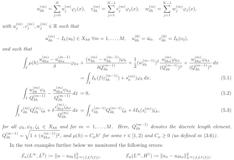
Problem 5.1 (Fully discrete scheme). Find functionsu(δhm)∈Xh andw(δhm), c (m)
δh ∈Xh0,m= 0, . . . , M, of the form
u(δhm)=
N
X
j=0
u(jm)ϕj(x), c(δhm)= N−1
X
j=1
c(jm)ϕj(x), w(δhm)= N−1
X
j=1
w(jm)ϕj(x),
with u(jm), c (m) j , w
(m)
j ∈Rsuch that
u(δhm)−Ih(ub)∈Xh0 ∀m= 1, . . . , M, u(0)δh = ˆu0, cδh(0)=Ih(c0), and such that
Z
I
µ(h)u
(m) δhx−u
(m−1) δhx
δ ϕhx+
(u(δhm)−u(δhm−1))ϕh
δQ(δhm−1) + 1 2(w
(m−1) δh )
2 u (m) δhxϕhx
(Q(δhm−1))3 +
w(δhxm)ϕhx
(Q(δhm−1))3dx
=
Z
I
Ih(f(c(δhm−1)) +s(um))ϕhdx, (5.1)
Z
I
wδh(m)ψh
Q(δhm−1) −
u(δhxm)ψhx
Q(δhm−1) dx = 0, (5.2)
Z
I
c(δhm)Q(δhm)ζh+δc (m) δhxζhx
Q(δhm) dx =
Z
I
c(δhm−1)Q(δhm−1)ζh+δIh(s(cm))ζh, (5.3)
for all ϕh, ψh, ζh ∈ Xh0 and for m = 1, . . . , M. Here, Q(δhm−1) denotes the discrete length element,
Q(δhm−1)=
q
1 + (u(δhxm−1))2, andµ(h) =C
µhr for somer∈[1,2)andCµ≥0 (as defined in (3.6)).
In the test examples further below we monitored the following errors:
Eu(L∞, L2) :=ku−uδhk2L∞(J,L2(I)), Eu(L
∞
, H1) :=kux−uδhxk2L∞(J,L2(I)),
Eu(H1, L2) :=kut−uδhtk2L2(J,L2(I)), Eu(H
1, H1) :=
kutx−uδhtxkL22(J,L2(I)),
Ew(L∞, L2) :=kw−wδhk2L∞(J,L2(I)), Ew(L2, H1) :=kwx−wδhxk2L2(J,L2(I)),
Ec(L∞, L2) :=kc−cδhk2L∞
(J,L2(I)), Ec(L2, H1) :=kcx−cδhxk2L2(J,L2(I)), (5.4)
where J = (0, T) and uδh has been extended by linearly interpolating on each time interval so that, for
instance, uδht= (u(δhm)−u (m−1)
δh )/δ fort∈(t(m−1), t(m)). We used sufficiently accurate quadrature rules
on each rectangle [t(m−1), t(m)]×[x
j−1, xj].
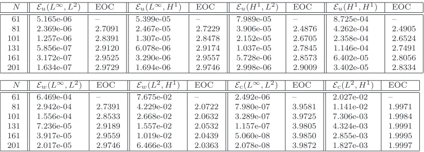
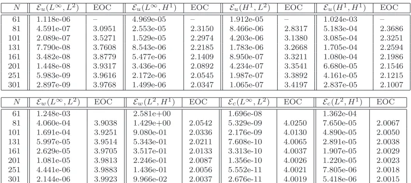
In a first example, letT = 1 and
f(c) =1−2c 10 , and consider
u(x, t) = 5
2cos(2πt)(x−1)
3x5,
c(x, t) = 1
10sin(7πx) sin(4πt).
(5.5)
The source functionssu(x, t) andsc(x, t) are picked such that the above functions solve (1.1)–(1.5). Note
that then ub= 0. We remark that the function uhas also been considered in [11].
[image:22.612.82.545.138.454.2]For varying values of N (h = 1/N, δ = h2) the errors and corresponding EOC’s are displayed in
N Eu(L∞, L2) EOC Eu(L∞, H1) EOC Eu(H1, L2) EOC Eu(H1, H1) EOC
61 5.454e-06 – 5.701e-05 – 8.398e-05 – 9.160e-04 –
81 3.258e-06 1.7910 3.389e-05 1.8080 5.271e-05 1.6193 5.696e-04 1.6516
101 2.155e-06 1.8524 2.236e-05 1.8637 3.600e-05 1.7087 3.870e-04 1.7315
131 1.310e-06 1.8967 1.357e-05 1.9042 2.258e-05 1.7777 2.417e-04 1.7941
161 8.779e-07 1.9283 9.081e-06 1.9334 1.544e-05 1.8306 1.649e-04 1.8426
201 5.683e-07 1.9490 5.874e-06 1.9524 1.018e-05 1.8680 1.085e-04 1.8771
N Ew(L∞, L2) EOC Ew(L2, H1) EOC Ec(L∞, L2) EOC Ec(L2, H1) EOC
61 6.840e-04 – 7.722e-02 – 2.492e-06 – 2.027e-02 –
81 4.060e-04 1.8129 4.361e-02 1.9864 7.992e-07 3.9536 1.141e-02 1.9971
101 2.677e-04 1.8660 2.796e-02 1.9908 3.299e-07 3.9647 7.306e-03 1.9984
131 1.624e-04 1.9055 1.657e-02 1.9938 1.165e-07 3.9690 4.324e-03 1.9991
161 1.087e-04 1.9341 1.095e-02 1.9958 5.108e-08 3.9693 2.855e-03 1.9995
[image:23.612.86.501.117.265.2]201 7.030e-05 1.9530 7.013e-03 1.9970 2.108e-08 3.9668 1.827e-03 1.9997
Table 1: Errors (5.4) and EOCs for the first test problem (5.5) described in Section 5 withµ(h) = 40h.
N Eu(L∞, L2) EOC Eu(L∞, H1) EOC Eu(H1, L2) EOC Eu(H1, H1) EOC
61 1.233e-05 – 1.289e-04 – 1.731e-04 – 1.882e-03 –
81 4.828e-06 3.2587 5.019e-05 3.2795 7.588e-05 2.8672 8.146e-04 2.9105
101 2.155e-06 3.6146 2.236e-05 3.6239 3.600e-05 3.3417 3.870e-04 3.3350
131 7.925e-07 3.8129 8.215e-06 3.8164 1.390e-05 3.6256 1.514e-04 3.5777
161 3.517e-07 3.9128 3.646e-06 3.9124 6.336e-06 3.7851 7.033e-05 3.6923
201 1.455e-07 3.9556 1.509e-06 3.9517 2.674e-06 3.8666 3.067e-05 3.7192
N Ew(L∞, L2) EOC Ew(L2, H1) EOC Ec(L∞, L2) EOC Ec(L2, H1) EOC
61 1.591e-03 – 8.962e-02 – 2.499e-06 – 2.027e-02 –
81 6.053e-04 3.3586 4.604e-02 2.3152 8.008e-07 3.9557 1.141e-02 1.9971
101 2.677e-04 3.6552 2.796e-02 2.2345 3.299e-07 3.9738 7.306e-03 1.9984
131 9.802e-05 3.8299 1.585e-02 2.1631 1.160e-07 3.9849 4.324e-03 1.9991
161 4.344e-05 3.9198 1.023e-02 2.1088 5.064e-08 3.9913 2.855e-03 1.9995
[image:23.612.86.501.318.466.2]201 1.796e-05 3.9589 6.442e-03 2.0733 2.077e-08 3.9947 1.827e-03 1.9997
Table 2: Errors (5.4) and EOCs for the first test problem (5.5) described in Section 5 withµ(h) = 4000h2.
N Eu(L∞, L2) EOC Eu(L∞, H1) EOC Eu(H1, L2) EOC Eu(H1, H1) EOC
61 5.165e-06 – 5.399e-05 – 7.989e-05 – 8.725e-04 –
81 2.369e-06 2.7091 2.467e-05 2.7229 3.906e-05 2.4876 4.262e-04 2.4905
101 1.257e-06 2.8391 1.307e-05 2.8478 2.152e-05 2.6705 2.358e-04 2.6524
131 5.856e-07 2.9120 6.078e-06 2.9174 1.037e-05 2.7845 1.146e-04 2.7491
161 3.172e-07 2.9525 3.290e-06 2.9557 5.728e-06 2.8573 6.402e-05 2.8056
201 1.634e-07 2.9729 1.694e-06 2.9746 2.998e-06 2.9009 3.402e-05 2.8334
N Ew(L∞, L2) EOC Ew(L2, H1) EOC Ec(L∞, L2) EOC Ec(L2, H1) EOC
61 6.469e-04 – 7.675e-02 – 2.492e-06 – 2.027e-02 –
81 2.942e-04 2.7391 4.229e-02 2.0722 7.980e-07 3.9581 1.141e-02 1.9971
101 1.556e-04 2.8533 2.668e-02 2.0632 3.289e-07 3.9725 7.306e-03 1.9984
131 7.236e-05 2.9189 1.557e-02 2.0532 1.157e-07 3.9805 4.324e-03 1.9991
161 3.917e-05 2.9559 1.019e-02 2.0439 5.060e-08 3.9850 2.855e-03 1.9995
201 2.017e-05 2.9746 6.466e-03 2.0363 2.078e-08 3.9872 1.827e-03 1.9997
[image:23.612.86.500.518.667.2]