Accreting neutron stars and black holes

(1)

A Thesis Submitted for the Degree of PhD at the University of Warwick

Permanent WRAP URL:

http://wrap.warwick.ac.uk/127764

Copyright and reuse:

This thesis is made available online and is protected by original copyright.

Please scroll down to view the document itself.

Please refer to the repository record for this item for information to help you to cite it.

Our policy information is available from the repository home page.

(2)

Accreting Neutron Stars and Black Holes

by

Zhuqing Wang

Thesis

Submitted to the University of Warwick

for the degree of

Doctor of Philosophy

Department of Physics

(3)

“A journey is a person in itself; no two are alike.

And all plans, safeguards, policies and coercion are fruitless.

We find after years of struggle that we do not take a trip; a trip takes us.”

(4)

List of Tables

1.1 A list of observed optically bright, active low-mass X-ray binaries . . . 24

3.1 Observations of V801 Ara and V926 Sco . . . 54

3.2 Revised system parameters for V801 Ara and V926 Sco . . . 64

3.3 Optical observations of GR Mus . . . 68

3.4 Revised system parameters for GR Mus . . . 75

3.5 System parameters for Aql X-1 . . . 80

4.1 XTE J1814-338 emission line parameters . . . 88

4.2 XTE J1814-338 system parameters . . . 104

5.1 Observations of Sco X-1 . . . 110

5.2 Sco X-1 system parameters . . . 125

6.1 A list of observed optically bright, active low-mass X-ray binaries with updated system parameters . . . 131

A.1 RVs determined from 1999 WHT observations . . . 137

A.2 RVs determined from 2011 WHT observations . . . 140

A.3 RVs determined from 2011 VLT observations . . . 144

(8)

List of Figures

1.1 Roche equipotential surfaces in the orbital plane for a binary system . . . . 3

1.2 Disc instability plot . . . 8

1.3 An artist’s impression of a typical low-mass X-ray binary . . . 9

1.4 X-ray burst profiles from 4U 1702 42 . . . 12

1.5 A cartoon depicting the evolution of a ZAMS binary system that results in a binary millisecond pulsar . . . 14

1.6 NS mass-radius curves for typical EOSs . . . 15

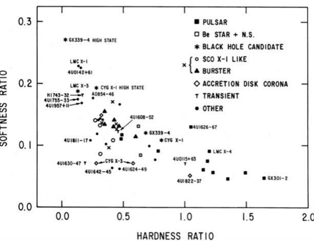
1.7 An X-ray color-color diagram taken from the High Energy Astronomy Ob-servatory 1 A-2 scanning data. . . 16

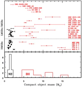
1.8 Masses of NSs and BHs measured in XRBs . . . 17

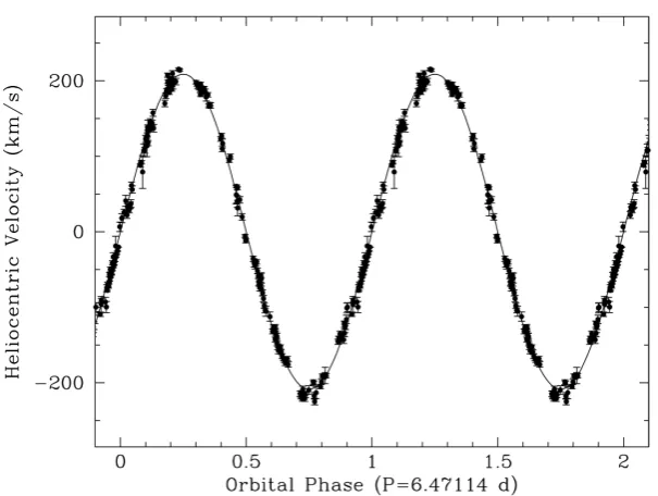
1.9 Radial velocity curve of the secondary star in V404 Cygni . . . 19

1.10 Trailed spectrogram of the Bowen blend and Heii 4686 for Sco X-1 . . . 21

1.11 Radial velocity curves of the sharp Bowen emission components and Heii 4686 emission line . . . 22

1.12 K-correction as function of the mass ratio for di↵erent disc opening angles . 23 1.13 Estimates for the gravitational wave strain amplitude (h0) for a number of known accreting neutron star sources as a function of frequency . . . 27

2.1 Example spectra from the 2011 VLT observations of Sco X-1 . . . 30

2.2 Trailed spectrogram of the Bowen blend for Sco X-1 and V926 Sco . . . . 32

2.3 Model contour map of the disc in velocity space . . . 33

2.4 Schematic view of a CV in both Doppler coordinates and spatial coordinates in the binary frame . . . 35

2.5 Doppler maps of GW Lib and the LMXB X1822-371 . . . 37

2.6 The MEM solution for a 2-pixel image . . . 39

2.7 Doppler maps of ASAS 0025+1217 . . . 40

2.8 2_{versus entropy trajectories (constant C} aim) . . . 42

(9)

2.10 Example bootstrap maps of J1814 338 . . . 44 2.11 Number distribution of the peak height of the donor emission spot

deter-mined from bootstrapped images of J1814 . . . 44 2.12 Number distribution of the peak height of a potential donor emission spot

determined from bootstrapped images of ASAS 0025+1217 . . . 45 2.13 Distribution of the goodness-of-fit level of synthetic maps . . . 46 2.14 Bowen Doppler images of Sco X-1 for an assumed parameter of 77,

113.6 and 150 km s 1 _{. . . 48}

2.15 Bowen Diagnostic diagram for Sco X-1 . . . 49 2.16 Plot of synthetic Kcor models for↵between 0 and 18 as a function of q

determined by our code . . . 50

3.1 Average Doppler corrected spectra of the Bowen region for the systems observed by our team during the period 1999 – 2005 . . . 52 3.2 Toolbox for Bowen data analysis. . . 53 3.3 Trailed spectra of the Bowen blend and Heii 4686 for V801 Ara and V926

Sco . . . 55 3.4 Bowen Doppler images of V801 Ara for an assumed parameter of 19,

31 and 81 km s 1_{. . . 56}

3.5 Number distributions of the phase shift, peak emission and Kemmeasured

from 2000 bootstrap maps of V801 Ara assuming = 31 km s 1 . . . 57 3.6 Bowen Diagnostic diagram for V801 Ara . . . 58 3.7 Bowen Doppler images of V926 Sco for an assumed parameter of 90,

140 and 190 km s 1_{. . . 59}

3.8 Number distributions of the phase shift, peak emission and Kemmeasured

from 2000 bootstrap maps of V926 Sco assuming = 140 km s 1 . . . . 60 3.9 Bowen Diagnostic diagram for V926 Sco . . . 61 3.10 The 68% and 95% confidence regions and projected PDF’s forK2andqfor

V801 Ara . . . 62 3.11 The 68% and 95% confidence regions and projected PDF’s forM1andM2

for V801 Ara . . . 63 3.12 The 68% and 95% confidence regions and projected PDF’s forK1,K2and

qfor V926 Sco . . . 65 3.13 The 68% and 95% confidence regions and projected PDF’s forM1andM2

(10)

3.16 Bowen Doppler images of GR Mus for an assumed parameter of 230, 180

and 130 km s 1_{. . . 70}

3.17 Number distributions of the phase shift, peak emission and Kemmeasured from 2000 bootstrap maps of GR Mus assuming =180 km s 1 . . . 71

3.18 Bowen Diagnostic diagram for GR Mus . . . 72

3.19 The 68% and 95% confidence regions and projected PDF’s forK1,K2and qfor GR Mus . . . 73

3.20 The 68% and 95% confidence regions and projected PDF’s forM1andM2 for GR Mus . . . 74

3.21 RVs of the Bowen emission components determined from the GTC and VLT observations of Aql X-1 . . . 77

3.22 The Doppler tomogram of Niii4640.64/4641.84 Å of Aql X-1 . . . 78

3.23 Distributions of the relative peak height and Kem determined from 2000 bootstrapped maps of Aql X-1 . . . 79

3.24 The Doppler tomogram of N iii 4634/4640 and C iii 4647/4650 of X1822 371 . . . 82

3.25 Number distributions of the phase shift, peak emission and Kemmeasured from 2000 bootstrap maps of X1822 371 assuming = 44 km s 1 . . . . 83

3.26 Bowen Diagnostic diagram for X1822 371 . . . 84

4.1 The average optical spectrum of XTE J1814-338 . . . 88

4.2 Trailed spectra of the strongest emission lines for XTE J1814-338 . . . 89

4.3 The diagnostic diagram of Heii 4686 for J1814 . . . 91

4.4 Doppler maps of the main spectral features for J1814 . . . 92

4.5 Number distributions of the phase shift, peak emission and Kemmeasured from 2000 bootstrap maps of J1814 assuming = 30 km s 1 . . . 94

4.6 Bowen diagnostic diagram for J1814 . . . 96

4.7 Constraints onqusing the K amplitude derived from the Bowen and Heii 5411 spot . . . 98

4.8 Average doppler corrected spectrum of the Bowen region for J1814 . . . 100

4.9 The 68% and 95% confidence regions and projected PDF’s forK2andqfor J1814 . . . 102

4.10 The 68% and 95% confidence regions and projected PDF’s forM1andM2 for J1814 . . . 103

4.11 A comparison of the mass-radius relationships for the companion of J1814 and 3 t-MSPs . . . 105

(11)

5.2 RVs of the Bowen emission components determined from the 1999 WHT, 2011 WHT and 2011 VLT observations of Sco X-1 . . . 114 5.3 The combined Doppler tomogram of the Bowen blend for Sco X-1 for the

1999 & 2011 WHT data . . . 115 5.4 Number distributions of the peak height, RV semi-amplitude and phase shift

determined from 2000 combined, bootstrapped images of Sco X-1 using

= 113.6 km s 1 . . . 116 5.5 Centre of symmetry method for Sco X-1 . . . 120 5.6 The 68 per cent and 95 per cent confidence regions and projected PDF’s for

K1,K2andqfor Sco X-1 . . . 123

5.7 The 68 per cent and 95 per cent confidence regions and projected PDF’s for M1andM2for Sco X-1 . . . 124

5.8 Simulated residual RVs obtained by subtracting the sinusoidal fit from the irradiation model . . . 127 5.9 Posterior PDFs for the apparent eccentricity derived from combined RV

data of Sco X-1 . . . 128

6.1 Impact of the quality of the ephemeris on GW searches during the A-LIGO era . . . 135

(12)

Acknowledgments

I would like to take this opportunity to wholeheartedly thank my supervisor, Danny Steeghs, for all his guidance and encouragement throughout this adventure. My gratitude goes also to Prof. Tom Marsh, for making the new softwares available, and for taking the time to answer my additional questions. Without their expertise and constant support, this work would not have been possible.

I would also like to thank my main collaborators: Jorge Casares, Duncan Galloway, Teo Mu˜noz-Darias, and Felipe Jim´enez-Ibarra. It was fantastic to have the opportunity to work with you. Thanks for providing the data that enabled me to carry out the work described here, and most importantly, for all your advice, patience and support.

To my fellow graduate students, Kristine, Chris and James for lots of little talks over the

co↵ee break and sharing your knowledge and experience. To my office mates, Odette, Mark and

David for being there whenever I needed advice, companionship, or distractions. With a special mention to Anna, who never fails to cheer me up. Thanks for making every day of work more interesting. I cannot wait to hear about your future adventures!

My special thanks go to all my housemates at #87. Katy & Maria: I miss our interesting chats and all the laughs we had. Lily & Shuwen for your signature cheese cake and fried chicken. Lisa & Rain who inspired me to start my plant-based journey. And Jenna for being a constant source of distraction. Best of luck for the road ahead!

To my dearest friends Aggie and Jessie. Thank you for taking chances and risks, both with me and in your own life.

And finally, to my parents, for everything you’ve done to inspire me at every stage of my

life, for putting up with my anxiety and silliness. Thank you, Dad, for being my greatest cheerleader.

(13)

Declarations

This thesis is submitted to the University of Warwick in support of my application for the degree of Doctor of Philosophy. It has been composed by myself and has not been submitted in any previous application for any degree. This thesis represents my own work except where stated otherwise.

Part of Section 3.3has been published in: Jiménez-Ibarra, F., Muñoz-Darias, T., Wang, L., Casares, J., Mata Sánchez, D. and Steeghs, D. et al.;Bowen emission from Aquila X-1: evidence for multiple components and constraint on the accretion disc vertical struc-ture; 2018, Monthly Notices of the Royal Astronomical Society, 474, 4717.

Chapter 4is based on: Wang L., Steeghs D., Casares J., Charles P. A., Mu˜noz-Darias T., Marsh T. R., Hynes R. I., O‘Brien K.;System mass constraints for the accreting millisecond pulsar XTE J1814-338 using Bowen fluorescence; 2017, Monthly Notices of the Royal Astronomical Society, 466, 2261. Observations and reduction of the VLT data were carried out by J. Casares.

(14)

Abstract

X-ray binary systems o↵er the best way to measure the masses of the accreting compact objects.

Following the discovery of the narrow Bowen emission lines in the prototypical low-mass X-ray binary, Sco X-1, arising from the X-ray illuminated atmosphere of the donor star, the Bowen

diag-nostic has been used as a general tool to obtain dynamical information for persistent sources and/or

transients during outburst. Here I exploit the Doppler tomography technique and develop Monte Carlo style bootstrap tests in order to obtain the most robust binary parameter constraints even in the low signal-to-noise ratio regime. Using a new set of analysis tools, I show that we can push the

limit of observations to moderately faint (B⇠19) persistent sources with 8-m class telescopes.

The method has also been applied to the case of the accreting millisecond X-ray pulsar XTE J1814 338, where the Bowen technique played a crucial role in the derivation of the radial

velocity of the secondary,K2. The resulting constraints on the binary component masses suggest

the presence of a ‘redback’ millisecond pulsar in XTE J1814 338 during an X-ray quiescent state. Sco X-1 remains the most important Bowen blend system for benchmarking our method as well as a critical target for continuous gravitational wave searches. I provide revised constraints on key orbital parameters in direct support of continuous-wave observations of Sco X-1 in the Advanced-LIGO era. In light of the new constraints on orbital parameters, the ranges of search parameters

T0and Porbshould be updated with the refined period and ephemeris. More importantly, the range

for the projected semi-major axis (axsini) needs to be expanded in order to cover the full parameter

space.

In the last chapter, I present a summary of the method and the key results of its application to

all 7 systems (including two transients). The list of Bowen targets can be expanded as new transient

outbursts are detected, which may provide us with the opportunities to find stellar-mass black holes.

Finally, I remark that the method developed in this thesis can be used to characterize other features

(15)

Abbreviations

ADC . . . Accretion disk corona

AMXP . . . Accreting millisecond X-ray pulsar

BH . . . Black hole

BHC . . . Black hole candidate

CoS . . . Centre of symmetry

CV . . . Cataclysmic variable

CW . . . Continuous-wave

DIM . . . Disc instability model

EOS . . . Equation of states

E-ELT . . . European Extremely Large Telescope

ESO . . . European Southern Observatory

FORS2 . . . FOcal Reducer and low dispersion Spectrograph 2

FWHM . . . Full width half maximum

GTC . . . Gran Telescopio Canarias

GW . . . Gravitational-wave

HJD . . . Heliocentric Julian Date

HMXB. . . High-mass X-ray binary

ISIS . . . Intermediate dispersion Spectrograph and Imaging System

LIGO . . . Laser Interferometer Gravitational–Wave Observatory

LMXB . . . Low-mass X-ray binary

MCMC . . . Markov–chain Monte Carlo

MEM . . . Maximum entropy method

MSP . . . Millisecond pulsar

(16)

OSIRIS . . . Optical System for Imaging and low-Intermediate Resolution Integrated Spectroscopy

RLOF . . . Roche-lobe overflow

RV . . . Radial velocity

RXTE . . . Rossi X-ray Timing Explorer

SNR . . . Signal–to–noise ratio

SXT . . . Soft X-ray transient

tMSP . . . Transitional millisecond pulsar

UTC . . . Universal time coordinated

UVES. . . Ultraviolet and Visual Echelle Spectrograph

VLT . . . Very Large Telescope

WHT . . . William Herschel telescope

(17)

Chapter 1

Introduction

Compact objects (white dwarfs, neutron stars and black holes) are the end-products of stel-lar evolution. A post-main sequence star will evolve to a red giant when its H-exhausted core exceeds the Sch¨onberg-Chandrasekhar limit after a period of Hydrogen shell burning. For stars less massive than⇠5M , the stellar core contracts down towards forming a white dwarf when contraction of the core is stopped by electron degeneracy. More massive stars fuse progressively heavier elements until iron builds up in the core and a supernova ex-plosion can be triggered when the mass of the star is greater than the Chandrasekhar limit of 1.44M (ignoring chemical composition). Once the central density exceeds⇠1012_kg

m 3_{, electrons will combine with protons to form neutrons and neutrinos that are packed}

(18)

1.1 Binaries

1.1.1 Roche geometry

For a binary system with massesM1andM2and separationa, the Roche potential including

the e↵ects of both the gravitational and centrifugal force is given by

(r)= GM1 |~r r~1|

GM2

|~r r~2|

1

2(~!⇥~r)2 (1.1)

where G is the universal gravitational constant,! is the angular frequency of the orbit (= 2⇡/Porb), and from Kepler’s third law,!2=G(M1+M2)/a3. The dimensionless form of the

Roche potential,

N(x,y,z)= ₍₁2

+q) 1 r1 +

2q (1+q)

1 r2 +

✓

x q

(1+q) ◆2

+y2, (1.2)

describes the shape of the potential surfaces, dependent only on the ratio of masses of the two components, q = M2/M1 < 1. While the binary separation a determines their sizes.

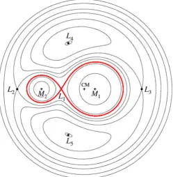
Figure 1.1 shows the equipotential surfaces of the Roche potential ( R(r) =constant) for a binary system withq = 0.25. Close to each component, the equipotential surfaces are nearly spherical as the gravitational potential of one of the component is dominant. Further outwards, the combined gravitational influence of M1 and M2 distorts the surfaces into

teardrop shapes.

There are 5 equilibrium points (L1toL5) where the gravity and the centrifugal force

cancel each other out (r R =0). The critical surface that envelopes both stars and joins at the inner Lagrangian pointL1(between the two stars) defines theRoche lobeof each star.

If one star starts to fill its Roche lobe (and the potential ofL1is lower thanL3), then matter

passing through the L1-point will move from a region where it is gravitationally bound

toM2 into the gravitational potential well ofM1. This process of transferring mass from

one star to the other is calledRoche-lobe overflow (RLOF). The equivalent radius1 _{of the}

secondary’s Roche lobe is approximated (to better than 1%) by

RL2

a

0.49q2/3

0.6q2/3₊ _ln(1₊_q1/3₎, 0<q<1 (1.3)

(Eggleton,1983), valid over the entire range of mass ratiosq; or

RL2

a 0.462 ⇣ q

1+q ⌘1/3

, 0.1_q_0.8 (1.4)

(19)

[image:19.595.197.447.225.480.2]

Figure 1.1: Lines of constant gravitational potential for a binary. Indicated are the positions of the primary and the secondary star and the center of mass of the system (CM). The equipotential surface that encloses both stars and intersects at a pointL1defines the Roche

lobe of each star (red). There are 5 equilibrium points (L1–L5) where the gravity and the

centrifugal force cancel out, and these are known as the Lagrangian points. If starM2fills

its Roche lobe, a particle passing through the first (or inner) Lagrangian pointL1will move

from a region where it is gravitationally bound toM2into the gravitational potential well of

(20)

(Paczy´nski,1971), which is accurate to a few per cent but more convenient than equation (1.3).

1.1.2 Binary evolution

The binary angular momentumJcan be expressed as:

J =M1M2

r Ga

M, (1.5)

whereM= M1 +M2is the total mass of the system. Di↵erentiating the expression for the

angular momentum, the rate of change in the binary separation can be derived as

˙ a a =

2 ˙J J

2 ˙M1

M1

2 ˙M2

M2 +

˙ M

M, (1.6)

and dots represent derivative with respect to time. The mass ratio, the orbital separation and the binary period changes during the periods of mass transfer, and stable mass transfer is subject to the balance between the loss of angular momentum, response of the donor to mass loss and changes of separation. Under the assumption that all the mass lost by one star is gained by the other and that the total angular momentum of the system is conserved ( ˙J=0), equation (1.6) becomes

˙ a a =

2 ˙M2

M2 (1 q). (1.7)

it is clear that the orbit expands (˙a>0) whenM2<M1(and ˙M2<0) while the binary shrinks

whenM2>M1. Further, using the expression for the secondary’s Roche lobe (equation 1.4),

the variation of the Roche lobe radius can be derived as: ˙

RL RL =2

˙ J J +2

˙ M2 M2 ✓₅ 6 q ◆ . (1.8)

Thus ifq<5/6 (and ˙J= 0), the size of the secondary’s Roche lobe will expand ( ˙R2 >0).

Sustained and stable mass transfer (which requires that the mass-losing secondary stays in touch with its Roche lobe) is possible if the system shrinks by losing angular momentum.

Three time scales are important for the study of binary evolution. The dynamical time scale over which a star responds to deviations from hydrostatic equilibrium:

⌧dyn=

r 2R3

GM (1.9)

(21)

to radiate away its gravitational energy:

⌧th= GM

2

RL (1.10)

The third time scale is the main sequence lifetime of a star:

⌧nuc⇡7⇥109yr M M

L

L (1.11)

The heavier star evolves more rapidly because the high mass stars have higher core temperatures and thus burn hydrogen more efficiently. Mass transfer will begin withM2>

M1, and when material is moved further away from the centre of mass, the stellar separation

has to be reduced. This decreases the Roche lobe size; the heavier star overfills its Roche lobe even more, driving further mass transfer. As the lower-mass companion is unable to adjust thermally to the accreted mass, the material overfills both Roche lobes. Within the cloud surrounding the binary components, the more massive star and the secondary spiral toward each other, simultaneously expanding and expelling the ‘common envelope (CE)’. Steady, long-lived mass transfer can occur when the donor expands to fill the Roche lobe due to stellar evolution; or the orbit, and thus the secondary’s Roche lobe, shrinks due to angular momentum loss. There are two main causes of angular momentum loss in a binary: magnetic braking and gravitational radiation.

Magnetic braking

A late-type secondary star filling its Roche lobe in a close binary system is expected to be tidally locked to the orbital period, forcing the star to co-rotate with the orbit. Ionised particles in the stellar wind are forced to follow the magnetic-field lines, and co-rotate with the secondary star. Since these lines are closed near the rotational equator, the particles are mainly released from the stellar poles (with large velocities), essentially extracting angular momentum from the binary orbit, which then shrinks, and the period decreases. A prescrip-tion for the angular-momentum loss due to magnetic braking is given byRappaport et al. (1983):

˙

JMB= 3.8⇥10 30M2R4

✓_R₂ R

◆

⌦3dyne cm, (1.12)

(22)

Gravitational Radiation

As binaries evolve to sufficiently short periods, gravitational radiation becomes a dominant source of angular momentum loss. According to Einstein’s general theory of relativity, matter curves space and the orbital motion of a binary system causes ripples in the fabric of space-time. The energy and angular momentum carried by these ripples is extracted from the binary orbit, causing the stars to spiral inwards, hence decreasing the orbital separation and period. General relativity predicts that the rate of angular momentum loss due to the emission of gravitational waves is described by:

˙

JGWR= 32₅ G

7/2

c5

M2

1M22M1/2

a7/2 (1.13)

Paczy´nski(1967), where c is the speed of light in a vacuum. Dense and compact objects like

neutron stars and black holes are strong distorters of space-time, and gravitational waves produced by orbiting pairs of these objects have been observed by the Laser Interferometer Gravitational-Wave Observatory (see Section 1.4).

1.1.3 Accretion discs

If the primary in asemi-detachedbinary (R?1<RL1andR?2>RL2) is a compact object, the

stream of gas lost from the companion star, viaL1, does not accrete directly onto the

pri-mary. The material will instead go into a circular orbit around it and settle at a distance Rcirc

(the circularization radius), at which the orbiting matter has the same angular momentum as its angular momentum at theL1point. Within the ring of gas, several dissipative processes

(e.g. collisions, shocks, and viscous dissipation) will take place, converting orbital energy into internal gas energy. Some of the energy is eventually radiated, and the material has to sink deeper into the gravity of the compact object (due to loss of kinetic energy). As the stream spirals inwards, a small amount of gas also moves outwards to conserve angular momentum. Anaccretion discis then formed. Matter is ultimately accreted onto the pri-mary from the inner layers of the disc. The outward expansion of the disc is disrupted at a maximum radius (rtidal), where tidal interactions with the mass donor removes the angular

momentum transported outwards and keeps the disk from overflowing the Roche lobe. For a schematic illustration of the disc formation process by RLOF, see Figure 1 fromVerbunt (1982).

The luminosity, Lacc, resulting from the accretion can be written as:

Lacc=⌘Mc˙ 2, (1.14)

(23)

matter into heat for a compact object of massM1and radiusR1, and ˙Mis the mass accretion

rate. The enormous gravitational field of neutron stars and black holes can yield much higher luminosities compared to what white dwarfs can produce from a given amount of in-falling material.

One of the most characteristic phenomena displayed by cataclysmic variables (that have a white dwarf and a normal star companion) and some of the low-mass X-ray binaries (soft X-ray transients; see Section 1.2.1) is the semi-regular outburst where their luminosity increases by several orders of magnitude. However, steady-state accretion flows cannot describe these time-dependent phenomena.Osaki(1974) suggested a cause for the outburst based on an instability in the accretion disc. The rationale is that if the mass transfer rate into the disc from the donor is higher than mass transfer rate through the disc onto the compact primary by viscous interactions, then material would pile up in the disc. For accretion discs with vertical heightH, the viscosity is parametrized as

⌫=↵csH, (1.15)

wherecs is the sound speed in the gas, and ↵. 1 denotes the size of the viscosity as a

fraction of the limiting case. The pile-up might eventually cause the disc to become un-stable, increasing the viscosity and angular-momentum transport, and spreading the excess material both inwards and outwards. The increased accretion onto the compact primary enhances the luminosity of the system and drains the disc of its material. The disc will then return to a quiescent, low-viscosity state. During quiescence, interaction between the gas stream and the disc causes the disc to gradually shrink (since the stream material has an-gular momentum corresponding to the circularisation radius, which is less than the specific angular momentum at the disc edge) until the next outburst occurs.

Disc instability

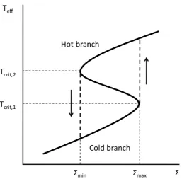
The transient behaviour can be understood as the ‘limit-cycle’ between the surface density and the surface temperature (or equivalently, the accretion rate through the disc) for an annulus of the disc (see Figure 1.2). The S-curve is the line of thermal equilibrium, where the viscous heating balances the radiation from the surface. On the branch with dTe↵/d⌃

< 0, for a small positive perturbation of ⌃, the annulus would have to seek equilibrium at a lower Te↵. However, a small increase in ⌃causes an increase in heating and hence

a movement away from the curve. Such a region is therefore unstable. In contrast, the branches with dTe↵/d⌃>0 are stable.

(24)

[image:24.595.193.451.108.361.2]

Figure 1.2: A plot of the disc’s surface density versus its surface temperature. The S-shaped thermal equilibrium curve forces the disc to follow the limit cycle, see text.

the low-mass X-ray binary lies on the lower branch. However, suppose that the rate of mass transfer arriving at the outer edge of an annulus is greater than ˙Mcrit,1, the surface

density will increase as the annulus cannot pass mass to inner annuli at the same rate as it receives it. Eventually the disc moves towards the maximum surface density⌃maxon the

lower branch. At this point, any further rise in⌃produces a runaway rise in temperature. Since the timescale for heating is far shorter than the time for viscous exchange of material, ⌃stays constant and the ring heats on a thermal timescale until a new equilibrium on the top branch of the S-curve is reached. Here however, with the condition ˙M < M˙crit,2, the

annulus evolves towards lower T until it reaches the left turning point at⌃min, where T and

˙

M must adjust on a thermal timescale again, cooling to the lower branch; and the whole cycle repeats.

In fact, an outburst is initiated in one annulus that reaches the critical surface density. The higher viscosity then spreads hot material into neighbouring annuli, sending heating waves inwards and outwards until most of the disc is on the upper branch. The transition into quiescence is triggered when the surface density is reduced to⌃minat some disc ring,

which is always in the outer disc (since⌃min is the highest here). This annulus returns to

(25)

Figure 1.3: An artist’s impression of a typical low-mass X-ray binary showing a compact object (either a neutron star or a black hole) accreting matter from a Roche-lobe filling low-mass companion star. (Credit: Rob Hynes).

1.2 Low-mass X-ray binaries

X-ray Binarieshave either a neutron star (NS) or black hole (BH) component, and can be separated into two main groups according to properties of the compact object’s companion star: high-mass X-ray binaries (HMXBs) and low-mass X-ray binaries (LMXBs), the main topic of this thesis. In high-mass X-ray binaries, the compact object accretes via a strong stellar wind from a massive star (M2&10M ; usually an O or B type, or a Be type

star), driven by the radiation pressure from photons escaping the star.

A low-mass X-ray binary has a low-mass secondary star (M2 . 2M ; typically

with spectral type G, K or M) that evolves to fill its Roche lobe, and transfers matter to the compact object through theL1 point in the form of a stream. The escaping material

(26)

1.2.1 X-ray transients

LMXBs can be divided into two populations based on their long-term behavior: those that accretepersistentlyat high mass-accretion rates (LX ⇠1036 erg s 1) and thetransient

sys-tems. LMXB transients (often referred to as soft X-ray transients; SXTs) spend most of their lives in a dim quiescent state (LX ⇠ 1030 – 1032 erg s 1), but undergo sporadic

out-bursts when their X-ray luminosity increases by several orders of magnitude on timescales of days to months (or years), making them indistinguishable from persistent sources.

The sporadic outbursts are thought to be triggered by thermal-viscous instabilities in the accretion disc that leads to an increased mass accretion rate onto the compact accretor (see e.g.Lasota 2001). Dynamical studies have shown thataccreting black holes are mostly found (& 70%) in transient LMXBs; whereas persistent LMXBs mostly contain neutron stars, as implied by the detection of coherent pulsations or bursts. The high incidence of BHs among XRTs is a consequence of the low mass transfer rates expected for their evolved low-mass companions. In BH binaries, the lack of a hard stellar surface in the compact star inhibits disc stabilization through X-ray irradiation (which di↵ers sharply for NS and BH systems) atlowaccretion rates (King et al.,1996,1997a,b). Thus the transient behavior of dynamical BH candidates (BHCs) appears to provide direct confirmation of the fundamental property of black holes (which is the lack of a material surface). Using a sample of 52 X-ray binaries, it was shown that the Disc Instability Model (DIM) modified by irradiation e↵ects could successfully explain the transient/persistent dichotomy (Coriat et al.,2012).

Transients are discovered during outburst by X-ray or ray all-sky monitors such as those on board GRO,Swiftand XTE. Monitoring of tens of known transients has allowed detailed studies of the spectral and timing properties over the outburst period. During peri-ods of quiescence when the optical brightness decreases by⇠7 magnitudes, the faint donor star may be entirely responsible for the optical flux. This o↵ers the best opportunity to perform radial velocity studies of the donor, thereby constraining the mass of the compact star (see Section 1.2.5). The main focus of this thesis is the mass measurements for systems in active states, which is possible via theBowen fluorescence technique. We will discuss in later chapters in depth the recent developments of the Bowen technique and the applica-tions to persistent LMXBs and/or transients in outburst to obtain robust dynamical system parameter constraints.

1.2.2 Neutron stars in low-mass X-ray binaries

(27)

be substantially narrower than that of LMXBs with neutron stars (White & van Paradijs, 1996), indicating that NS systems receive much larger kick velocities (when they are born in a supernova) than BH systems may have obtained. If the NS system remains bound after the supernova kick, a binary with a low-mass companion will receive a larger systemic kick than a binary with a high-mass companion (e.g.Brandt & Podsiadlowski 1995;van Paradijs & White 1995). During their lifetime, the systems with the low-mass companion and a long lifetime (⇠107_{– 10}9_{yr) will travel further away from their birth place (assuming they are}

born in the Galactic plane) compared to X-ray binaries with a high-mass companion and a much shorter lifetime (105_{– 10}7_yr).

Many NS-LMXBs exhibit type I X-ray bursts due to unstable thermonuclear burn-ing on the surface of the neutron star (Lewin, van Paradijs, & Taam,1993,1995). The start of the X-ray burst is extremely rapid, with the X-ray flux increasing by at least an order of magnitude (usually within a second) in all energy bands. This is followed by an exponential decay (due to the cooling of the radiating material), lasting from a few seconds to minutes, and persists for a longer time at lower energies (see Figure 1.4 for example Type I burst profiles).

Swank et al.(1977) noted that for a particular burst the X-ray spectrum was best

fitted by a cooling blackbody. Assuming a distance of⇠ 5–10 kpc, the blackbody radius required to radiate the observed X-rays in the cooling tail of the burst was estimated to be in the range 10–15 km (consistent with the size of a neutron star). Therefore, the radiation observed during the X-ray burst must arise from the surface of the compact object, which must be a neutron star. As a sufficient amount of hydrogen accretes onto the neutron star, an underlying surface layer of helium will be built up (via nuclear fusion) due to the extreme conditions prevailing. Once a critical density and temperature in the helium layer is reached, it also starts burning (fusing into carbon), giving rise to an explosive thermonuclear flash of X-ray emission. Once the burst is over, the NS continues to accrete fresh hydrogen and re-accumulate the helium layer, and another burst will be generated after a similar amount of time. The recurrence time between the X-ray bursts ranges from hours to days (but occasionally minutes) depending on the mass accretion rate.

(28)

Figure 1.4: (Type I) X-ray burst profiles from 4U 1702 42 observed with EXOSAT in the 1.2–5.3 keV band (left) and the 5.3–19.0 keV band (right). The burst persists for a longer time at lower energies (it has a cooling tail). Taken fromvan Paradijs(1998).

‘Z-sources’ (for the characteristic Z-shaped pattern that the spectral variations trace in the X-ray color-color diagram;Hasinger & van der Klis 1989).

1.2.3 Millisecond pulsars

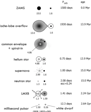
Figure 1.5 illustrates the evolutionary scenario for the formation of an LMXB, and eventu-ally the formation of a binary millisecond radio pulsar, from an initial binary containing a massive supergiant and a low-mass star (.1M ). Since the radius of the progenitor of the compact object must be much larger than the present size of the LMXB, the system must therefore lose a large amount of angular momentum during its evolution (e.g. Kalogera & Webbink 1998). As described in Section 1.1.2, the more massive star evolves much faster than its companion and is the first to fill its Roche lobe. The mass transfer time scale (dictated by the thermal or dynamical time scale of the supergiant) is considerably shorter than the time scale on which the low-mass companion can adjust thermally to the accreted mass. Consequently, the accreted layer will heat up, and the secondary will expand to fill its Roche lobe, thereby forming a common envelope which engulfs the binary. With the formation of the CE, the secondary rapidly spirals towards the core of the primary due to frictional dissipation. As energy is dissipated in the common envelope, the envelope ex-pands and is eventually ejected from the system. The stripped helium core of the progenitor then undergoes a core-collapse supernova explosion to form a NS primary.

(29)

phase is initiated when mass starts flowing from the secondary towards the neutron star. Mass transfer is driven either by the expansion of the mass donor or shrinkage of the orbit due to angular momentum loss from the system. Depending on the nature of the secondary, the physical mechanism responsible for angular momentum losses may be magnetic braking and/or gravitational radiation.

Since the discovery of the first millisecond radio pulsar (MSP;Backer et al.,1982), it has been suspected that long periods of mass transfer onto old NSs hosted in LMXBs might be responsible for spinning up the compact object to the ms regime. A ‘recycled’ MSP is thought to be formed when accretion turns o↵completely (Alpar et al.,1982). The detection of the first accreting millisecond X-ray pulsar (AMXP) SAX J1808.4-3658 in the course of an X-ray outburst episode (Wijnands & van der Klis,1998) provided a nice confirmation of the recycling scenario. The radio pulsar/LMXB link was firmly confirmed with more recent discoveries of transitional millisecond pulsar binaries. The most notable examples include the ‘missing link pulsar’ PSR J1023+0038 that turned on as an MSP after an LMXB phase (Archibald et al., 2009); and the direct evolutionary link IGR J18245-2452, which has shown both an MSP and an AMXP phase (Papitto et al.,2013); and XSS J1227.0-4859 (see, e.g.,de Martino et al. 2014;Roy et al. 2015).

The most precise neutron star masses can be determined from several relativistic e↵ects on the pulse arrival times of double NS systems (e.g. Wolszczan 1991;

Arzouma-nian 1995;Nice et al. 1996). Accurate mass determinations have also been obtained for

(30)

[image:30.595.163.477.185.571.2]

(31)

[image:31.595.160.479.107.350.2]

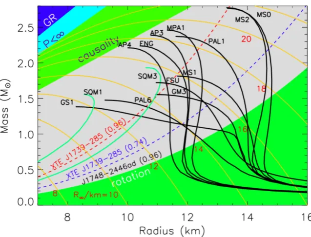
Figure 1.6: Mass-radius curves for neutron stars for typical EOSs (black) and strange quark matter EOSs (green). Taken fromLattimer & Prakash(2007).

(Lattimer & Prakash,2004,2007).

Each available equation of state provides a mass-radius relation for a fixed core density (see Figure 1.6), and the maximum possible NS mass (Mmax

NS ) is a function of the

assumed EOS (Mmax

NS ⇠ 1.5 M forsoft EOSs and up to ⇠ 2.7 M for the sti↵est EOS).

Most EOS curves involving exotic particles (that predict a maximum mass well below 2 M ) are already ruled out. More mass measurements can help reveal even higher mass NSs (see, e.g., the recent constraint byLinares, Shahbaz, & Casares 2018). The e↵ect of rapid rotation can raise the upper limit up to 20% (Friedman et al.,1986). If the mass is greater than'3.2 M , then a black hole is formed.

1.2.4 Black hole candidates

(32)

[image:32.595.167.474.104.339.2]

Figure 1.7: An X-ray color-color diagram taken from the High Energy Astronomy Obser-vatory 1 A-2 scanning data. The spectra are averaged over a& 5 day interval. Cyg X-1 was only observed in the low state; the high-state values were estimated from the high-state spectra given inSanford et al.(1975).

additional emission from a boundary layer in the NSs (Done & Gierli´nski,2003). In spite of the fact that some X-ray spectral characteristics of BHs are also seen in some NSs, the combined presence of these spectral characteristics and rapid variability of the X-ray flux has remained e↵ective in identifying black hole candidates in new transient sources.

Reliable BH masses have been measured in⇠ 22 XRBs. These are displayed in Figure 1.8 along with the observed NS masses. The fact that NS masses tend to be higher in LMXBs than in HMXBs could be a manifestation of the pulsar recycling scenario. Neu-tron stars in HMXBs are less modified by accretion and thus their masses lie closer to the birth values. Figure 1.8 also shows that there is a gap (between⇠2–5M ) in the current distribution of compact remnant masses (see alsoFarr et al. 2011). This property contrasts with numerical simulations byFryer & Kalogera(2001) – including mass loss from stellar winds and binarity e↵ects – which lead tocontinuousmodel distributions. The discrepancy may be caused by selection e↵ects since low-mass black holes might be hiding among other X-ray sources, although several XRBs (e.g. LS 5039, 4U 1957+115 and GX 339 4) have been reported to contain BHs with masses likely between 2–5M (Casares et al., 2005;

Gomez et al.,2015;Heida et al., 2017). However, on the other hand, if the mass gap is

(33)

[image:33.595.184.462.108.404.2]

Figure 1.8: Masses of neutron stars (black) and black holes (red) measured in X-ray bi-naries (Top). Observed mass distribution of compact objects in X-ray binaries (Bottom). Taken fromCasares, Jonker, & Israelian(2017).

depends solely on the growth timescale of the instabilities driving the explosion of massive stars. Instabilities that develop within the first⇠10–20 ms after the bounce and leads to a rapid explosion within 200 ms of the initial stellar collapse can account for the data. For slower-growing turbulent instabilities, significant fallback is expected and compact objects with masses falling between the observed gap are predicted.

(34)

1.2.5 Dynamical mass measurements

With two stars orbiting about the common centre of mass, we haveM1/M2=a2/a1, where

Mis the stellar mass,ais the distance between the stellar components. As observed at an inclinationi, the orbital velocity (K) projected along the line of sight is

K1 = 2⇡a1

Porb sini and K2 =

2⇡a2

Porb sini (1.16)

for the primary and the secondary star, respectively. Combining equation (1.16) and Ke-pler’s law (and usinga=a1 M1_M+₂M2), we can obtain the mass function

f(M)= K

3

2 Porb

2⇡G = M3

1sin3i

(M1+M2)2 =

M1sin3i

(1+q)2, (1.17)

whereq=M2/M1=K1/K2is the mass ratio of the binary components. With measurements

of the two observablesK2and Porb, equation (1.17) gives the absolute minimum allowable

mass of the compact primary (sini.1 and 1+q>1). Therefore, a mass function in excess of⇠3M (the upper limit of the NS mass for any standard EOS) is widely considered as the best signature for a BH.

When an X-ray transient fades into quiescence (corresponding to the lowest accre-tion rates), the contribuaccre-tion to the optical light by the accreaccre-tion disc significantly decreases, which may o↵er the best opportunity to directly detect the faint low-mass companion and probe its nature. The Doppler shift of narrow absorption lines from the donor (as it moves around the centre-of-mass) provides information aboutK2, the absolute phase zero, and the

systemic velocity ( ). Figure 1.9 shows an example radial velocity curve of the donor star in V404 Cyg, obtained by cross-correlation of photospheric absorption lines with the rest wavelength spectrum (of a star of similar spectral type to the companion). Spectroscopic analysis during quiescence revealed a K0 companion star of V404 Cyg moving with a ve-locity amplitude of 211 km s 1_{in a 6.5 d orbit. These two parameters alone imply a mass}

function of f(M)=6.26±0.31M , well above the upper limit of the NS mass. Hence, the compact objectmustbe a BH. This result is so remarkable, as it marks the first unambigu-ous discovery of a stellar mass BH, where no additional assumptions on the inclination nor M2need to be invoked.

As mentioned above, the mass function represents only a lower limit to the mass of the compact object, M1. Precise measurements of the stellar masses also require the

(35)

[image:35.595.170.473.104.332.2]

Figure 1.9: Radial velocity curve of the secondary star in V404 Cygni. The radial velocity semi-amplitudeK2=211±4 km s 1 and the orbital period 6.473±0.001 d yield a mass function of f(M)=6.26±0.31M . Adapted fromCasares et al.(1992).

ratio ofK2to the rotational broadening of absorption lines (Vrotsini) can be approximated

by a function ofq:

Vrotsini

K2 '0.462

⇥₍₁₊_q₎2_q⇤1₃ _(1.18)

(Wade & Horne,1988)2_{. Therefore the usual step towards finding the mass ratio is via the}

determination of Vrotsini.

The rotational broadening can be measured by comparing the spectrum of the Roche-lobe-filling secondary with that of a slowly rotating single star, and determine the optimal broadening that is required for the template to be matched to the target spectrum (through 2

minimization; see e.g.Marsh et al. 1994;Casares & Charles 1994). The rotationally broad-ened versions of the template are computed by convolution with a limb-darkbroad-ened rotational profile (Gray,1992).

Lastly, we need the constraint oni(which can be reliably measured only in eclips-ing systems) to calculate the true value of the compact object massM1. For a few systems,

the binary inclination has been inferred from the orientation of radio jets (e.g. Sco X-1,

Fomalont et al. 2001; GRS 1915+105,Steeghs et al. 2013). However, in most cases, the

(36)

2002). In practice, there are sources of contamination that can seriously distort the true ellipsoidal modulation (e.g. near-quiescence super-hump waves, the hot spot, and flaring activities). Worse still, the cubic dependence of the mass function equation on the inclina-tion angle means that uncertainties on the final mass soluinclina-tion are largely dominated by the errors ini. Thus the search for the relatively rare eclipsing systems (that might be hidden from our view) is needed, in order to obtain more accurate estimates foriand henceM1.

1.3 The Bowen fluorescence technique

The detection of donor star signatures in many LMXBs has remained difficult for decades. For many systems the companion is too faint to study even during quiescence. Sources with bright optical counterparts tend to be the persistent ones, where the mass accretion rate is high. In these active systems, the optical emission is dominated by the reprocessing of hard X-rays in the outer accretion disc, this obviously hampers direct detection of the much fainter companion. For persistent LMXBs or transients during outburst, the use of Bowen emission lines – first discovered in the prototypical LMXB Scorpius X-1 – as tracers of the companion’s motion provides the only opportunity to constrain their system parameters.

1.3.1 Detection of the mass donor in Sco X-1

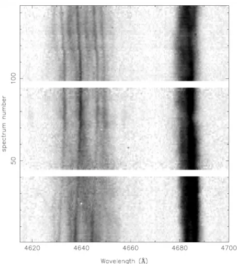
Sco X-1 is one of the brightest optical LMXBs harboring a neutron star that accretes mat-ter from a Roche lobe-filling companion at high accretion rates. Phase-resolved, resolution spectroscopy of Sco X-1 led to the first discovery of extremely narrow, high-excitation emission components in the Bowen region (4630-4660Å), mainly consisting of a blend of Niiiand Ciiilines. These narrow line features show significant Doppler motions as a function of orbital phase, as can be seen from a 2-D trailed spectrogram (Figure 1.10). Closer inspection of the trailed spectra revealed at least 3 narrow Niii/C iii components moving in phase with each other, but in anti-phase with respect to the underlying broad component.

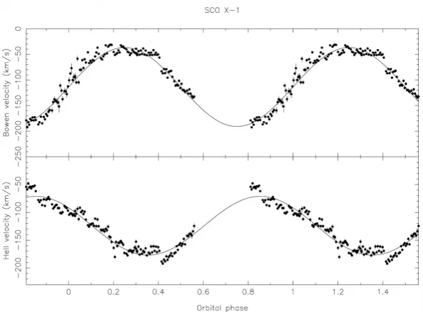
The radial velocity (RV) variation of the Bowen emission blend can be derived from multiple-Gaussian fitting to individual spectra, which gives the (common) velocity of the three sharp components and its formal error. The resulting radial velocity curve is shown in Figure 1.11 (upper panel), together with that of the Heii 4686 emission line (lower panel) based on a double-Gaussian fit.

(37)

[image:37.595.198.443.105.378.2]

Figure 1.10: Trailed spectrogram of the Bowen blend and Heii 4686 for Sco X-1. At least 3 narrow lines within the broad Bowen region can be seen to be present at all orbital phases. Figure fromSteeghs & Casares(2002).

Further support for the hypothesis of donor origin can be drawn from the comparison of the RV curves in Figure 1.11. The blue-to-red crossing point in the RV curve of the narrow lines occurs near the phase of minimum light, at which we face the (un-irradiated) backside of the donor and the visibility of the X-ray heated side of the secondary is minimum. This is therefore the first-ever direct detection of the mass donor in luminous LMXBs. On the other hand, the almost anti-phased line wings of Heiiemission can be attributed to the accretion flow around the compact object, note that a phase delay of⇠ 0.1 – 0.2 with respect to the inferior conjunction of the primary is observed in this case (likely due to residual hot spot contamination).

1.3.2 Parameter constraints via the donor signature

(38)

[image:38.595.172.469.105.324.2]

Figure 1.11: Radial velocity curves of the sharp Bowen emission components (top) and Heii 4686 emission line (bottom). Best-fit sinusoidal waves are overplotted as solid lines. Figure fromSteeghs & Casares(2002).

Since we are using emission line diagnostics (instead of the conventional absorption line) and the narrow Bowen components originate from the irradiated front face of the mass donor, the derived Kemvelocity must be biased towards lower values, i.e., Kem< K2(see

e.g. Figure 1.3). In order to transform the measured Kemamplitude to the true velocity of

the centre of mass of the companion K2, the so-calledK-correctionneeds to be applied to

Bowen blend RVs.

By generating synthetic RV curves using simulated emission line profiles formed by (isotropic) radiation on the illuminated hemisphere, the deviation between the reprocessed light centre and the centre of mass of the Roche-lobe-filling donor (Kcor=Kem/K2<1) can

be extracted.

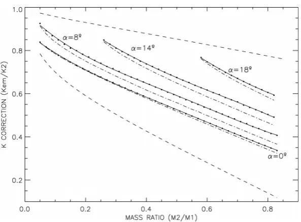
Mu˜noz-Darias et al.(2005) presented numerical solutions for Kcor(see Figure 1.12)

in their extensive study of K-correction modelling. Their main conclusion is that K-correction depends strongly on:

(i) the mass ratio, q=M2/M1;

(ii) disc flaring angle,↵, which represents the disc shadowing e↵ect.

The dependence on the inclination angleiis rather weak. Figure 1.12 plots the K-correction as functions ofqfor both high- (solid lines) and low-inclination angle cases (dash-dotted lines).

(39)

[image:39.595.173.470.101.320.2]

Figure 1.12: K-correction as function of the mass ratio for di↵erent disc opening angles. Kcor is at the minimum when↵=0 (i.e., maximum correction is required), and approaches

unity as↵increases. Figure fromMu˜noz-Darias et al.(2005).

is formed at the inner Lagrange point L1, thus only provides a purely theoretical limit.

The K-correction is e↵ectively constrained between ↵ = 0 when disc shielding can be neglected (maximum displacement), and the geometric limit set by emission from the limb of the irradiated region (minimum displacement; upper dashed line). E↵orts have been made to obtain knowledge of↵(for a system whereK2is known) from direct spectroscopic

measurements and detailed modelling (Jim´enez-Ibarra et al.,2018).

1.3.3 The Bowen survey

(40)

Table 1.1: A list of observ ed optically bright, acti ve lo w-mass X-ray binaries. Estimates of Kem and masses of the accretor were collated from pre viously published w orks using the Bo wen blend diagnostics. System Type Mag Porb Kem M1 Reference (hr) (km / s) ( M ) Sco X-1 Persistent B = 12.2 18 . 9 77 . 2 ± 0 . 4 > 0.2 Stee ghs & Casares ( 2002 ) X1822-371 Persistent B = 15.8 5 . 6 300 ± 8 1.6 2.3 Casares et al. ( 2003 ) GX 9 + 9 Persistent B = 16.8 4 . 2 230 ± 35 > 0.2 Cornelisse et al. ( 2007b ) V926 Sco Persistent B = 17.9 4 . 7 226 ± 22 > 0.5 Casares et al. ( 2006 ) LMC X-2 Persistent B = 18 8 . 1 351 ± 28 > 0.9 Cornelisse et al. ( 2007c ) V801 Ara Persistent B = 18.2 3 . 8 277 ± 22 > 0.8 Casares et al. ( 2006 ) GR Mus Persistent B = 19.1 3 . 9 245 ± 30 1.2 2.6 Barnes et al. ( 2007 ) GX 339 4 a Transient V > 21 42 . 1 317 ± 10 > 6.0 Hynes et al. ( 2003 ) Aql X 1 b Transient V ⇠ 22 19 . 0 247 ± 8 > 1.6 Cornelisse et al. ( 2007a ) XTE J1814 338 c Transient / AMXP V = 23.3 4 . 2 345 ± 19 > 1 Casares et al. ( 2004 )

Notes. a W

(41)

1.4 Gravitational waves

Over the past two decades, interferometric gravitational-wave (GW) detector technology has dramatically improved and now reached sensitivity levels that are sufficient for direct detection of GWs from astrophysical sources. On February 11, 2016, the first detection of the GW signal (GW150914) emitted from a relativistic in-spiral and merger of two large black holes was reported by the Laser Interferometer Gravitational Wave Observatory (LIGO)3 _{and the Virgo}4 _{collaboration (Abbott et al.,}_{2016), opening a new observational}

window for studying astrophysical objects. The subsequent detection of a binary neutron star merger (GW170817;Abbott et al. 2017b) confirmed the excitement of detecting GW transients and demonstrated opportunities for discovering new GW source types in the ad-vanced detector era.

It is therefore timely to target also a di↵erent GW signal: continuous waves (CWs) emitted by spinning neutron stars in LMXBs that may be detectable in the band of ground-based interferometric observatories. The expectations for CW gravitational radiation from LMXBs arise from the cut-o↵observed in the spin frequency distribution (of both LMXBs and millisecond radio pulsars) at around 700 Hz, well below the breakup limit (Chakrabarty

et al.,2003;Patruno,2010). Given the estimated ages (⇠1010_{yrs) and observed accretion}

rates of LMXBs, accretion is expected to spin up the NS to at least>1 kHz (for standard NS equations of state;Cook et al. 1994). Thus, there should exist some braking torque to bal-ance the spin-up from accretion. One possibility is the loss of angular momentum through gravitational radiation (Papaloizou & Pringle,1978;Wagoner,1984;Bildsten,1998). If a NS is asymmetric with respect to its rotation axis, it will emit a CW with frequency f at a given ratio with respect to the star rotational frequency⌫s. Di↵erent mechanisms were

proposed to describe how a small asymmetry in the neutron star might be developed: e.g., crustal mountains (f=2⌫s;Bildsten 1998;Ushomirsky et al. 2000;Melatos & Payne 2005;

Haskell et al. 2006); magnetic deformation (f = 2⌫s; Cutler 2002; Haskell et al. 2008);

and internal r-mode oscillations (f ⇡4/3⌫s;Andersson 1998,2003). Assuming a balance

between the accretion torque and the spin-down torque by the GW radiation, the expected GW signal strength at the Earth can be expressed as:

h0⇡4⇥10 27

✓ _F_X

10 8_{erg cm} 2_s 1

◆1/2✓_{300 Hz}

⌫s

◆1/2

, (1.19)

whereh0= L/L is the strain, i.e., the fractional change in length of an interferometer arm, andFX is the incident X-ray flux. Note that the⌫s1/2 scaling arises only because of the

(42)

torque balance (Lasky, 2015). The most promising targets for periodic GW searches are then the brightest sources with the lowest spin frequencies.

Depending upon thea prioriknowledge of the target source, searches for continu-ous gravitational waves generally fall into three broad categories: 1)targetedsearches in which the star’s position and rotation frequency are precisely known (e.g., known radio, X-ray or -ray pulsars); 2)directed searches where the direction of the source is known but little or no frequency information is available (e.g., non-pulsing LMXBs) and 3)all-sky searches for unknown neutron stars (Riles, 2017). The volume of parameter space over which to search increases by large steps as one progresses through these categories and, for 2) and 3), any unknown binary orbital parameters (if a star is in a binary system) fur-ther increase the search volume. Without accurate determinations of the orbital parameters, an observational ‘penalty’ must be paid. E↵ectively, the signal must be proportionately stronger, compared to a source where the parameters are more precisely constrained, in order to reach the same order of confidence for a detection.

Many directed GW searches on known LMXBs have been carried out, mainly fo-cusing on the potentially most luminous source of continuous GW radiation for LIGO and VIRGO, Sco X-1 (Figure 1.13; see alsoMeadors et al. 2016;Abbott et al. 2017a;Meadors et al. 2017). Since in these cases the source strengths are expected to be small, one must integrate data over long observation times to have any chance of signal detection. So far, only upper limits on the signal amplitude have been obtained (2.3⇥ 10 25 _{for Sco X-1;}

Abbott et al. 2017c). In general, the greater knowledge one has about the source, the more computationally feasible it is to integrate data coherently (preserving phase information) over long observation times. Thus, improvements in the precision of the system parame-ters of candidate persistent GW sources are essential for reducing the volume of parameter space that needs to be searched, which will contribute to computationally cheaper searches and eventually allowing the use of the most sensitive types of approaches (Messenger et al., 2015).

1.5 Goals of this study

(43)

[image:43.595.171.473.225.478.2]

Figure 1.13: Estimates for the gravitational wave strain amplitude (h0) for a number of

(44)

in active LMXBs. Our new analysis toolsets will then be applied to several systems in-cluding the 5th_{accreting millisecond X-ray pulsar XTE J1814-338, which can yield results}

o↵ering insights into the evolutionary scenario involving binary pulsars. Furthermore, we will continue working to improve the precision of the key orbital parameters of Sco X-1 (our Bowen blend benchmark as well as the prime target for continuous GW searches) required by directed searches for continuous waves.

The rest of this thesis is structured as follows: Chapter 2describes the develop-ments of the analysis tools for obtaining dynamical system parameter constraints for Bowen targets.Chapter 3presents the (re-)analysis of Bowen datasets using the newly developed Monte Carlo tools and provides updated binary parameter constraints of five LMXBs. In

Chapter 4, we apply the method to the 5th _{accreting millisecond X-ray pulsar (AMXP)}

(45)

Chapter 2

Methods

2.1 Data analysis

2.1.1 Radial velocity technique

Line profile fitting

We use themgfitroutine within themollyspectral analysis package1to fit Gaussian profiles to emission lines in time-resolved, continuum-normalised spectra. The tool allows for a simultaneous fit of multiple lines, and computes the peak height, the FWHM and the o↵set (relative to the rest wavelengths) of each component following the non-linear least squares fitting technique ofMarquardt(1963). Figure 2.1 shows the results of multiple-Gaussian fits to the three strongest narrow lines Niii 4634 & 4640Å and Ciii 4647 in the Bowen blend of Sco X-1.

It is known that during certain phase ranges, especially near phase zero 0(defined

as the inferior conjunction of the mass donor), the narrow emission lines from the donor could be much weaker than at other phases. In order to pick up weak features near phase zero (see, e.g., lower panel of 2.1), we can optimize the fitting code to take into account the spectrum-to-spectrum variation. For each spectrum, the expected RV of the narrow lines can be calculated (if the orbital phase is known) and used as the initial fit value of the velocity o↵set to guide the optimizer to a reasonable optimum (as was implemented to fit both spectra in 2.1). The quality of individual Gaussian fits should also be assessed by visual inspection, especially for spectra taken near the inferior conjunction of the companion.

(46)

(47)

Circular orbit fit

Assuming that the reprocessed light centre traces the orbit of the companion, and that the intrinsic eccentricity of the binary orbit is negligible (e = 0), the simplest model for the variation of the projected Bowen RVs is a sinusoid of the form

V(t)= +Ksin

✓_2⇡(_{t T}₀₎ Porb

◆

= +Ksin(2⇡( 0)), (2.1)

where is the RV of the system (systemic velocity), K is the measured velocity semi-amplitude, T0 is the epoch of inferior conjunction of the mass donor, Porb is the orbital

period (see Figure 1.11 for an example RV curve). To fit the 4 free parameters (T0, Porb, K,

and ), a least-squares method can be used and each data point is weighted according to the associated error bar given bymgfit. This method of extracting orbital parameters is referred to as the RV technique.

The well-established RV method has completely failed in most other cases where the signal-to-noise ratio is low, and the narrow components are too weak to be detectable in individual spectra. In Figure 2.2, we compare the trailed spectrogram of the Bowen blend for Sco X-1 and a fainter source in Table 1.1 (V926 Sco). The narrow ‘S-wave’ components arising from the heated hemisphere of the donor star can be clearly identified in the excep-tional Sco X-1 case, where we have shown the evolution of the Bowen blend as a function of orbital phase. The Bowen region of V926 Sco looks extremely complicated, probably dominated by many weak and blended S-wave features. In a case like this, there might still be genuine signal from the donor. Nonetheless, two outstanding questions remain: 1. Is there a way to extractKemfrom such noisy datasets? 2. (If yes) how do we estimate the

statistical uncertainty in the measuredKem?

2.1.2 Doppler tomography

(48)

Bowen$data$

Donor$emission$

Sco$X>1$

V926$Sco$

24'

Figure 2.2: Trailed spectrogram of the Bowen blend for Sco X-1 (left; all spectra are from 2011 WHT observations of Sco X-1, as presented inGalloway et al.(2014) and V926 Sco (in 50 phase bins;right).

The principle

The line profile expected from a simple Keplerian disk is broadened by the large velocities of the emitting gas. The contribution of a particular location is Doppler shifted due to its RV relative to the observer. If Doppler-shifting is the dominant broadening mechanism, all emission from within a region of more-or-less equal RV will contribute to the corresponding part of the velocity-resolved line profile (see Fig. 1 ofMarsh & Horne 1988). Hence a spectrum contains information on the integrated flux over the accretion region. Indeed, a line profile observed at a particular orbital phase can be seen as a collapse of the velocity-space image of the accretion flow at an angle defined by the phase. Fig. 2.3 gives an example of such an image in velocity space with an artificial spot of emission. From the two line profiles shown in Fig. 2.3, it is easy to locate the position of the spot by tracing back the peaks in the profile along the projection direction. In light of the idea of the CAT-scanning process, it is not hard to imagine that if a sequence of spectra is taken, ideally covering at least a whole orbital period, visualizations of the line-forming region can then be reconstructed in the form of a tomogram invelocity (or Doppler) coordinates.

To do this, we begin with a starting image and derive the equivalent trailed spectra. The modelled spectra are then compared against the observed spectra by a 2 _{statistic. In}

this way, the image can be modified iteratively until the predicted data is consistent with the observed data. The resultant image is given by auniquesolution that reaches a reasonable goodness-of-fit level (i.e. small 2_{, defined by the user) and occurs with maximum image}

entropy (i.e. the smoothest reconstruction).

(49)

Figure 2.3: Model contour map of the disc in velocity space (i.e. lines of equal radial velocity are straight). The spot is seen to be projected into di↵erent parts of the two example profiles at orbital phase 0.25 (right-most) and 0.5 (lower). The line profile at each orbital phase can then be recognized as the projection of the image along the line of sight. Figure is taken fromMarsh & Horne(1988).

=Ii/PjIj, selects the most uniform of all possible images. This could be a problem in the

case of the distribution of line emission which is generally a strong function of radius and is far from uniform. Doppler tomography instead uses a modified version of entropy that finds the most axisymmetric distribution consistent with the image, and allows the radial dependence to be determined by the data. The modified version ofS is given by

S =

n

X

i=1

pilogpi

qi, pi= Ii

P

jIj

, and qi = PJi jJj

, (2.2)

(50)

The Doppler coordinate system

As a point-like emission source (in the binary system) traces a sinusoidal radial velocity curve (as a function of orbital phase) around the system’s mean velocity ( ),

V( )= Vxcos2⇡ +Vysin2⇡ (2.3)

this eventually causes an S-shaped pattern (S-wave) that is frequently seen in 2-D trailed spectrograms. Depending upon the phase and amplitude of the S-wave, auniquecoordinate can be assigned to this point source, expressed by a velocity vector (Vx,Vy), relative to the inertialframe. This coordinate system has the advantage that it allows blended S-waves to be mapped into clear and separate features in the velocity space image.

We note that there are good reasons fornottrying to produce Doppler tomograms in the Cartesian xy-plane, as this would require unjustified assumptions being made (e.g. Keplerian flow in the disc) in order to translate between velocity and position. Worse still, there is often the danger that one point in the system can produce emission at more than one velocity, e.g., the stream-disc impact region. Given the close relationship between the velocity profile of emission lines and the accretion structure in velocity coordinates, we shall restrict ourselves to reconstructing maps in the velocity space. To get a good handle on Doppler maps, one must first get used to this special coordinate system.

In the Doppler coordinate frame, theVx-axis is conventionally defined by the

direc-tion from the accreting compact object to the mass donor, theVy-axis points in the direction

of motion of the donor star, and the centre of mass of the system is at the origin. Based on this definition, we can predict where key components in binary systems would end up in the reconstructed maps.

Understanding the map

Assume the system’s mean velocity is zero2_{, the centre of mass of the system does not move}

with respect to the observer, therefore appears on the map at (Vx,Vy)=(0, 0). In the case of the Roche-lobe-filling donor star, which is assumed to beco-rotatingwith the binary (v= !_^rfor ‘solid-body’ rotation), the transformation preserves the shape of the Roche lobe, but rotates its position to the positiveVy-axis of the tomogram (as the secondary star moves

in the positive y-direction by definition). The primary is also on theVy-axis, but below the

origin at (0, -K1).

A key point to realize is that the familiar picture of the accretion disc in spatial coordinates (Fig. 2.4,left) gets turned inside-out in velocity coordinates (Fig. 2.4,right).