How Do Sell-Side Analysts Obtain P/E Multiples to Value Firms?
Yuan Yin (Corresponding Author) Independent Scholar E-mail: yuanyin78@gmail.com
Ken Peasnell Professor of Accounting
Lancaster University Management School Lancaster, LA1 4YX
United Kingdom
E-mail: k.peasnell@lancaster.ac.uk
Herbert G Hunt III Professor of Accounting Orfalea College of Business
California Polytechnic State University San Luis Obispo, California 93407, United States
E-mail: hghunt@calpoly.edu
1
How Do Sell-Side Analysts Obtain P/E Multiples to Value Firms? Abstract
Previous studies of analysts’ valuation methods show that sell-side analysts often rely on multiples-based relative valuation methods in deriving target price forecasts, predominantly earnings-based multiples. However, little is known about how analysts actually arrive at the earnings multiples that they apply in their valuations. Based on extant valuation theory, we analyse three benchmarks/reference points that analysts use to select these multiples using U.S. data. By mimicking analysts’ relative valuation processes, we show that analysts tend to assign earnings multiple premiums (discounts) to those firms expected to have growth premiums (higher risk levels) relative to comparable firms. We provide evidence that analysts use firms’ historical earnings multiples as benchmarks, and assign firms that are expected to have more (less) attractive fundamentals than they have had in the past earnings multiples that are at a premium (discount) relative to the average historical earnings multiples at which they traded. The forward P/E multiple for the broad U.S. market index signals the market’s expectations about the growth prospects of the U.S. economy and future economic conditions and we also find that changes in this multiple affect analysts’ choices of firm-specific earnings multiples.
2
1. Introduction
Finance theory suggests that the value of a financial security is equal to the present value of the
cash payoffs that an investor in that security expects to receive (Palepu and Healy 2013).
Accordingly, it is not surprising that standard valuation textbooks place considerable emphasis
on present value models. It has been shown, however, that security analysts often use earnings
multiples-based valuation methods in practice (Cascino et al. 2014). As key information
intermediaries, sell-side analysts play an important role in promoting the efficient allocation of
financial resources in capital markets, but we have limited knowledge regarding how analysts
actually use the multiples method.
There are two main steps involved in applying the P/E multiple valuation method; the first
involves choosing comparable firms and the second is to determine the earnings multiple for the
firm under appraisal (the target firm). Graham and Dodd’s Security Analysis (1951, p. 507) states
that ‘The selection of an appropriate capitalization rate for expected earnings is just as important
in the determination of a common stock’s investment value as is a correct forecast of earnings.
The two might be called the primary determinants of value’. However, despite its importance in
the valuation process, the procedure of selecting an appropriate P/E multiple has received scant
attention from researchers, who often simply adopt industry average multiples and focus on the
selection of comparable firms (e.g., Bhojraj and Lee 2002, Liu et al. 2002, Nissim 2013).
Some progress has been made recently. Using hand-collected data from a small sample of
analyst reports, Yin et al. (2014) show that the P/E multiples applied by analysts to value firms
(i.e., analyst target P/E multiple)1 are positively associated with their near-term and long-term
earnings growth forecasts and negatively associated with risk measures such as financial
3
leverage and book-to-market. However, since the sample in that study comprises only 321
research reports issued by six brokerage firms for 260 firms for less than two years (October
2010 to March 2012), it remains an open question as to whether the results are generalizable to
the wider population of U.S. security analysts and firms or to a longer time frame.2 Most
importantly, there are two questions essential for the understanding of analysts’ multiples-based
valuations that remain unexplored. First, how do analysts determine the magnitudes of the P/E
multiples that they apply to value the firms they follow? While knowing that higher expected
earnings growth (risks) warrants a higher (lower) earnings multiple (Yin et al. 2014) is
important, ultimately analysts need to obtain the earnings multiples which they can then apply to
their earnings forecasts. Second, what, if any, practical mechanisms and techniques do analysts
employ to help obtain the appropriate P/E multiples for target firms? The present study attempts
to seek answers to these two questions by examining three P/E multiple benchmarks (i.e.,
comparable firms’ average, long-term historical average, and the market index’s multiple) which
analysts appear to use in their valuations.
Ohlson and Juettner-Nauroth’s (2005) theoretical model suggests a positive (negative)
relationship between a firm’s intrinsic forward P/E multiple and the firm’s near- and long-run
expected earnings growth rates (the cost of capital). We follow Ohlson and Juettner-Nauroth
(2005) and Graham and Dodd (1951) (hereinafter referred to for brevity as OJ and GD,
respectively) in our identification of pertinent variables. Our research design includes using
proxies for analyst target P/E multiples that we obtain through reverse engineering the analysts’
valuation procedures, by dividing the target price forecast by the capitalized earnings per share
4
estimate (provided that the P/E multiple is the method used). This approach allows us to examine
a large sample of U.S. firms across different economic sectors.
The results of our study show that by using the average P/E multiples of comparable firms as
benchmarks, analysts appear to assign P/E multiple premiums to firms with growth premiums in
the next fiscal year and in the medium-term, relative to comparable firms. They also seem to
assign P/E multiple discounts to firms with higher levels of risk (e.g., earnings volatility,
financial leverage). Firms with higher growth prospects relative to their long-run historical
averages receive higher P/E multiples from the analysts than the average historical P/E multiples
at which they traded. The results show that firms with increased levels of financial risk and stock
price volatility, compared to their long-run averages, are assigned lower P/E multiples relative to
the average P/E multiples at which they have historically traded. Finally, we find that revisions
in analyst target P/E multiples are positively associated with changes in the forward P/E
multiples of the Standard and Poor’s 500 Composite Stock Index (S&P 500 Index), suggesting
that analysts’ valuations incorporate information embedded in the market benchmark P/E
multiples.
This study contributes to our knowledge of how analysts perform the P/E valuation method
and, more generally, to the accounting-based valuation literature in several ways. First, we add to
the literature by revealing how analysts use comparable firms’ forward P/E multiples and target
firm’s historical P/E multiples as benchmarks to determine the magnitudes of earnings multiples
that they apply to value firms. These findings stand in sharp contrast to the textbook prescription
of universal application of an industry average. Second, to our knowledge, this is the first
large-sample study to empirically investigate how analysts select P/E multiples that are justified by
5
using analyst survey data. Third, our results provide additional support for the finding in Yin et
al. (2014) that analysts apply the P/E multiple valuation method in ways that are consistent with
the OJ theory that the P/E multiples are positively associated with the near-term and long-run
growth rates in future earnings. While we also find that financial statement measures, earnings
stability and financial leverage affect analysts’ choices of P/E multiples, the effect of high past
profitability and past growth appears to be rather limited. Fourth, we provide additional evidence
on analysts’ risk analyses in the context of their relative valuations. Fifth, this research is one of
only a few studies (e.g., Bradshaw 2004; Yin et al. 2014) that shed light on analysts’ decision
processes by examining the relationships among multiple analysts’ outputs. This study therefore
adds to our knowledge of analysts’ valuation activities, both by showing that what they do is not
simply a result of applying ad hoc procedures but rather can be reconciled with what prior work
suggests should be the relationship between stock valuations and accounting variables and the
part played by their assessments of risk.
The remainder of the paper is organized as follows. The next section reviews related studies,
Section 3 presents our hypotheses and Section 4 presents our empirical design. Sections 5 and 6
describe our sample and present empirical results. Section 7 presents additional empirical
analysis. Section 8 reports results of sensitivity analyses and Section 9 presents concluding
comments.
2. Related research
Over sixty years ago, GD suggested that equity investment decisions should be based on a formal
appraisal of the value of the business following a thorough study of all available facts (e.g.,
6
estimate of the average expected earnings for the subsequent five to ten years (i.e., the earnings
power).3 The value of the business can then be estimated by applying to the earnings estimate a
capitalization rate/multiplier that takes account of expectations about the business’s growth
prospects in the longer run. They go on to identify two categories of determinants of the earnings
multiple: one that includes easily measurable variables and another that includes non-measurable
intangibles. The first category includes factors such as profitability, progress (e.g., past growth),
earnings stability and financial strength, all of which can be determined by examining the firm’s
financial statements. The intangible factors are those that would be expected to influence, and
probably control, the firm’s long-run growth prospects including the nature and future prospects
of the target firm’s industry, the firm’s relative standing in the industry, and the quality of the
firm’s management team.
OJ show that under fairly general conditions the value of an equity security can be expressed
as being equal to the capitalized one-year-ahead earnings per share plus the present value of
capitalized abnormal earnings growth in all future periods:
∑
∞ =+ −
+
=
1
1 1
0
t
t t
E
r AEG R
r EPS
V (1)
where: E
V0 is the value of an equity security at date t = 0; r is the cost of equity capital; R is the
discount factor, equivalent to 1 plus the cost of capital, r; and
(
)
[
t t]
t
t eps eps r r dps
AEG+1 = +1− 1+ − ⋅ is abnormal earnings growth, defined as the change in
EPSadjusted for the cost of capital and dividends (dpst). To formalize growth in the equation,
7
the authors introduce a measure of growth in expected EPS in period t = 2, 𝑔𝑔23F
4. Assuming AEG
grows at a constant compound rate of (γ − 1) after period t = 2, OJ show that the intrinsic
forward P/E multipleis dependent on a near-term growth rate in expected EPS, 𝑔𝑔2, a long-run
growth rate in abnormal earnings growth, γ − 1, and the cost of capital, as follows: 5,6
(
)
(
1)
1
1 2
1 0
− −
− − × =
γ γ
r g r eps
VE
(2)
Little empirical evidence exists on how analysts deal with risk in security analysis. At least
two survey studies have reported that most analysts do not believe (or are at least not willing to
admit that they believe) in the Efficient Market Hypothesis and the CAPM (Block 1999, Barker
1999b). These findings should not be surprising since, unlike investment texts, analysts do not
assume the market is efficient (Penman 2013). Lui et al. (2007) suggest that analysts’ perception
of risk is multidimensional. They show that risk ratings issued by Salomon Smith Barney (now
known as Morgan Stanley Smith Barney) are associated with risk measures identified in the
literature such as idiosyncratic risk, leverage, size and book-to-market risk proxies, and earnings
quality. Peasnell et al. (2016) report a negative relationship between analysts’ stock
recommendations and stock price volatility. Both studies find that the effect of market beta is
mixed.
A number of studies have shown that earnings-based multiples (e.g., P/E, EV/EBITDA) are
the most popular valuation methods used in practice (Cascino et al. 2014). Imam et al. (2008)
4𝑔𝑔
2= [ ]. 𝑔𝑔2 captures the usual measure of EPS growth in FY2. It also reflects
an adjustment for foregone earnings as a result of dividends distribution (dps1).
5 For a firm that pays out all its earnings as dividends, it can be shown that (γ − 1) equals the long-run growth rate in the firm’s expected earnings per share.
8
examine UK analysts’ use of valuation models by interviewing a sample of 35 sell-side and
seven buy-side analysts and by analysing 98 research reports issued by the interviewees over the
period 2000-2003. The authors report that analysts perceive that the importance of the discounted
cash flow model (DCF) has significantly increased over time and is greater than reported in early
survey studies. The results of their content analysis provide support for this finding.
Nevertheless, they find that the importance of P/E multiple continues, and that valuation
multiples rather than DCF are relied on for the determination of target prices. Peasnell and Yin
(2014) examine 200 Investext research reports of U.S. firms issued by analysts of leading
brokerage firms in 2011-2012 and find that earnings multiples are used for the determination of
target prices in 60 per cent of the reports while DCF is used in only 18 per cent of the reports. In
short, prior research shows that earnings multiples remain the most frequently used method in
analysts’ valuations, at least in the U.S., although the use of DCF may have increased over time.
3. Hypotheses development
We formulate three hypotheses based on the theoretical work of GD and OJ, evidence from
broker reports, and recent empirical findings on analysts’ risk analyses. Analysts normally
provide one- and two-year ahead earnings per share forecasts (EPS1 and EPS2,respectively) and
an estimate of earnings growth for the next three to five years (i.e., long-term growth forecasts).
While expectations about growth in future earnings beyond the three to five-year forecast
horizon likely affect analysts’ target P/E multiples, such information is not available to
researchers and, thus, is omitted from our empirical analyses. It is important to note that the
analyst’s relative valuation approach likely captures at least partially the elements (industry
9
earnings growth beyond analysts’ forecast horizon since the average forward P/E multiples of
comparable firms should reflect the market’s view of the industry’s long-run growth prospects.
Furthermore, within the analyst industry coverage universe, stronger and more successful firms
are expected to receive higher P/E multiples.
Lui et al. (2007) and Peasnell et al. (2016) identify several factors that appear to play a role in
analysts’ risk adjustments and we include the most important of these as explanatory variables in
this study. The variables include stock price volatility, size and book-to-market risk proxies, and
financial leverage. Although empirical evidence of the effect of market beta on analysts’
decisions is mixed, because of its theoretical importance and long history as a measure of
riskiness, we include it in our empirical analysis.
In their research reports, analysts often provide explanations for why they issue earnings
multiple premiums/discounts for specific firms within their industry coverage universe. For
example, the following excerpt was taken from an Investext report on Pfizer provided by Credit
Suisse First Boston analysts:
This target P/FE (price to forecasted earnings multiple) considers the company’s growth outlook compared to that of its peers – a stronger outlook justifies a premium while a weaker outlook a discount. Pfizer’s growth prospects are the second lowest in the U.S. Major Pharmaceutical Group, and we assign a 25% relative P/FE discount to drug group peers.7
Based on prior literature and broker reports, we predict that, within the analyst’s industry
coverage universe, firms with higher growth in expected earnings will receive higher price-future
earnings multiples, while riskier firms will receive lower price-future earnings multiples.
Valuation textbooks (e.g., Penman 2013) suggest that one of the key steps of multiples-based
valuation is applying an average or median of the comparable firms’ multiples to the target
10
firm’s earnings forecast to obtain its value estimate. Some researchers (e.g., Lundholm and Sloan
2013) argue that the relative valuation approach incorporates little information about expected
future payoffs on which the value of the business hinges. If analysts subscribe to this textbook
approach and naively apply industry average multiples, we would not be able to observe the
relationships we predict. Hypothesis 1 (in alternative form) is thus:
H1:Within the analyst’s industry coverage universe, the valuation (P/E multiple) premium
that a firm receives is an increasing function of its growth premium relative to
comparable firms and a decreasing function of its excess riskiness relative to
comparable firms.
In terms of specific indicators of future profitability, GD suggest that readily measurable
factors such as past profitability, progress, and stability are among the likely determinants of
earnings multiples.8 We predict that a firm’s more favourable showing on these variables will
result in higher earnings multiples. Thus, Hypothesis 1a (in alternative form) is as follows:
H1a:Within the analyst’s industry coverage universe, firms with better past profitability, past
growth, and more stable earnings receive valuation (P/E multiple) premiums relative to
comparable firms.
GD suggest that a logical approach to selecting the earnings multiple is to study past
multiples, and either accept or modify them. However, they stress that analysts should avoid
using historical multiples without careful consideration because a firm’s prospects and quality
can change dramatically over time and, importantly, the analyst must assess the accuracy of the
market’s valuation.
11
Evidence from broker reports suggests that analysts examine both historical earnings
multiples and comparable firms’ forward P/E multiples. For example, a Morgan Stanley (2007)
research report states that it is more useful to understand not just how a stock valuation compares
to its peers, but whether the stock is under- or over-valued within the historical context. We
hypothesize that firms that are expected to have more (less) attractive fundamentals than their
historical records, such as higher growth rates in expected earnings and lower expected risks,
will be assigned target P/E multiples that are at a premium (discount) to their long-run historical
averages. Hypothesis 2 (in alternative form) is as follows:
H2: Firms that are expected to have stronger (weaker) fundamentals than they have had in
the past will receive premium (discounted) P/E multiples relative to their average
historical market P/E multiples.
To test these hypotheses, we follow prior practice and specify our main regressions such that
the dependent variable is not the P/E multiple premium but rather its reciprocal, the E/P multiple
premium. We do this for two reasons. First, this approach facilitates comparison with prior
research. Beaver and Morse (1978) and Zarowin (1990) motivate the use of E/P in part because
they derive it from Litzenberger and Rao (1971) where the relationships between E/P and growth
and risk are linear. Second, we use E/P to minimise scaling problems. White (2000) and Dudney
et al. (2008) use E/P because it is better behaved in a statistical sense: when the scaling variable
approaches zero, it can result in very large outliers that distort the regression relationship.9
9 As an untabulated sensitivity test, we re-estimate the regressions in the study using analyst target P/E multiples (as opposed to the inverse E/P measures used in our main tests) as the dependent variables. We eliminate
observations with negative EPS1 forecasts. We also eliminate a small portion of observations with the lowest (2, 3, and 5 per cent) EPS1 forecasts in an attempt to minimize the scaling problems (i.e., very large outliers) that might arise when the scaling variable EPS1approaches zero in the calculation of analyst target P/E multiples. The
12
4. Variables and Empirical Models
4.1 Variable definitions
We obtain a proxy for analyst target P/E multiple �𝑃𝑃�𝑡𝑡+1⁄𝐸𝐸𝑃𝑃𝐸𝐸1�by dividing the analyst’s
(typically, one-year-ahead) target price forecast,Pˆt+1,by her EPS1 forecast, both issued at date t
and collected from the Institutional Brokers' Estimate System (I/B/E/S). This allows us to
generate a large dataset of proxies for analyst target P/E multiples that would not be possible if
we hand-collected analyst target P/E multiples from broker reports.Some researchers suggest
that analyst choices of valuation methods may vary by economic sector (e.g., Barker 1999b,
Demirakos et al. 2004). Overall, however, evidence on the type(s) of multiples analysts apply to
value firms by industry is rather limited. Consequently, we do not have sufficient evidence to
exclude firms in certain industries from our sample. Importantly, our review of analyst reports
reveals that in the case where the P/E multiple is not the dominant valuation method, analysts
frequently appear to use the P/E multiple method to triangulate the target price forecast derived
from other valuation methods. We conduct our main empirical tests for both the pooled sample
and subsamples of economic sectors.
We examine two measures of analysts’ earnings growth forecasts: analysts’ long-term
growth forecasts (LTG) and their near-term growth forecasts (G2). G2 is calculated using the
formula:
(
EPS2 −EPS1)
/EPS1.We examine the following risk measures: financial leverage (LEV), measured as the total
liability-to-total assets ratio; stock price volatility (VOL), measured as the annualized standard
deviation of historical daily returns over the prior twelve-month period; size (Size), measured as
the natural logarithm of market value; the book-to-market ratio (B/M); and market beta (Beta),
13 over the prior sixty months.
We measure past profitability, stability, and past growth using the gross margin ratio at the
beginning of the EPS1 forecast period(GM)10, earnings volatility in the last five years (Earnvol),
measured as the standard deviation of the past five years’ earnings before extraordinary items
deflated by total assets, and the actual sales growth rate in the last five years(AGsales),
respectively. We calculate AGsales by fitting a least squares growth line to the logarithms of six
annual sales observations.
The OJ model assumes that there is no relation between a firm’s dividend payout policy and
its P/E ratio, consistent with the early work of Miller and Modigliani (1961). Since an analyst’s
forecasted target price represents her best estimate of the stock’s price at the end of the forward
twelve-month period, it is an ex-dividend value estimate. Ceteris paribus, analysts likely assign
lower P/E multiples to firms with higher dividend yields to adjust for the expected reduction in
the firm’s value resulting from dividends distribution. Thus, we include analyst forecasted
dividend yield (DY) as a control variable in our models.11
10 The review of broker reports and evidence in Peasnell and Yin (2014) suggests that analysts frequently use the gross margin ratio to forecast future earnings by multiplying forecasted sales by the gross margin ratio to obtain forecasted gross profit. Based on this evidence, we use gross margin ratio to measure past profitability in this study. Return on Equity (ROE) and the operating gross margin ratio would also be possibilities here. However, ROE exhibits a strong mean reversion tendency over the long run due to competition (e.g., Freeman et al. 1982, Fama and French 2000). Hence, it may act as a proxy for the expected future profitability in our tests, and therefore may not be suitable for testing GD’s assertion relating to the positive effect of past profitability on target P/E multiples. The operating gross margin ratio exhibits weaker mean reversion tendency than ROE, possibly due to the fact that technology and cost structure differ across industries (Nissim and Penman 2001), but it is also less stable and less useful than the gross margin ratio for forecasting earnings. As a sensitivity check, we re-ran all our empirical tests using both ROE and the operating gross margin ratio to measure past profitability. We find that analyst E/P multiple premiums are positively associated with the industry average-adjusted ROE and the operating gross margin ratio, suggesting that those measures acted more like proxies for future profitability. We interpret the results as suggesting that analysts expect future profitability of firms with high past ROE and operating gross margin ratio to revert to the mean (decay) over the long run and therefore issue higher target E/P multiples. We find similar results when ROE and the operating gross margin ratio are used in the historical average-adjusted tests.
14
4.2 Model for assessing analysts’ relative valuations based on comparable firms
We test Hypothesis 1 by examining the relationships between the E/P multiple
premiums/discounts firms received from the analysts, and their growth and risk premiums
relative to comparable firms. To analyse Hypothesis 1a, we examine whether firms that
outperform comparable firms in terms of past profitability, progress, and stability (PPS) receive
premium E/P multiples relative to comparable firms. Therefore, if we let i denote the target firm,
and θi denote the corresponding comparable group (i.e., the combination of firm i and its
comparable firms), and let j be the index of firms belonging to the comparable group , we can
analyse the relationships in Equation (3) as follows:
(3)
where 𝐸𝐸𝐸𝐸𝐸𝐸1,𝑖𝑖𝑖𝑖
𝐸𝐸�𝑖𝑖+1,𝑖𝑖𝑖𝑖 denotes the analyst target E/P multiple assigned to firm i at date t, calculated based
on the EPS1 and target price forecasts of firm i issued by the analyst at date t. 𝐸𝐸𝐸𝐸𝐸𝐸1,𝑗𝑗𝑖𝑖
𝐸𝐸𝑗𝑗𝑖𝑖 is the
forward E/P multiple of firm j, calculated by dividing firm j’s one-year-ahead earnings per share
forecast issued in the date t calendar quarter, EPS1,jt, by firm j’s current price,Pjt. Growthit
represents the expected earnings growth rate of firm i at date t, Riskit represents the expected
riskiness of firm i at date t, and PPSit represents firm i’s past profitability, progress and stability.
The dependent variable in Equation (3) is the difference between the analyst target E/P
multiple of firm i and the average forward E/P multiple12 of firms in the comparable group
and, as such, represents the E/P multiple premium that firm i receives from the analyst. The
12 Our reading of broker reports suggests that, in estimating industry average multiples, analysts do not appear to use the ‘out-of-sample’ approach. We therefore follow this practice and adopt the ‘in-sample’ approach for our empirical analysis here.
15 variableGrowthit meanj
{
Growthjt}
i θ
∈
− represents the expected growth premium of firm i relative to
its comparable firms, Riskit meanj
{
Riskjt}
iθ
∈
− represents the relative excess riskiness of firm
i, and 𝑃𝑃𝑃𝑃𝐸𝐸𝑖𝑖𝑡𝑡− 𝑚𝑚𝑚𝑚𝑚𝑚𝑚𝑚𝑗𝑗∈𝜃𝜃𝑖𝑖�𝑃𝑃𝑃𝑃𝐸𝐸𝑗𝑗𝑡𝑡� represents the past profitability, progress, and stability of firm i
relative to comparable firms.
We use I/B/E/S data to construct a proxy for the analyst industry coverage universe (the
comparable group). Analysts generally specialize in only a limited number of industries and a
relatively small number of firms (e.g., Boni and Womack 2006). As such, firms within an
analyst’s industry coverage universe should be deemed to be the relevant set of comparable firms
(Alford 1992, Boni and Womack 2006). Boni and Womack (2006) suggest that industry
divisions based on the third level of the S&P/MSCI Global Industry Classification Standard
(GICS) – ‘Industry’ – provide a good proxy for how firms are covered by analysts. We therefore
designate firms with the same third-level GICS code and covered by the same analyst as a
comparable group. We then compute the E/P multiple premium, the growth premium, and the
excess riskiness of firm i relative to its comparable firms, and similar relative measures of gross
margin ratio, sales growth, and earnings volatility in three steps.
First, we divide observations with target price forecasts issued by individual analysts along
three dimensions, by analyst, by third-level GICS industry code, and by calendar year-quarter, in
order to obtain analyst-industry-calendar quarter combinations. Our sample indicates that
analysts, on average, issue four target price forecasts per firm per year. We choose one calendar
quarter as the time span for the calculation of comparable group means.
Second, for each analyst-industry-calendar quarter unit that contains at least three distinct
firms, we calculate: (1) the mean forward E/P multiple for the comparable group,
𝑚𝑚𝑚𝑚𝑚𝑚𝑚𝑚𝑗𝑗∈𝜃𝜃𝑖𝑖 �
𝐸𝐸𝐸𝐸𝐸𝐸1,𝑗𝑗𝑖𝑖
16
margin ratio, the actual five-year sales growth rate, and earnings volatility for the comparable
group, with each firm equally weighted where multiple observations of a firm fall within the
same calendar quarter. For ease of notation, the resulting means are referred to as industry means
rather than comparable group means. We require the number of comparable firms (including the
target firm) in an analyst-industry-calendar quarter combination to be at least three, which is a
compromise between (1) having enough observations to avoid excessive noise, and (2) not
unduly reducing the sample size. We require each analyst-industry-calendar quarter to have
industry means greater than zero for all variables, a condition necessary for the calculation of
percentages in the next step.
Third, our methodology requires that we construct a measure of the E/P multiple premium
that is comparable across firms and analysts. Thus, we compute a percentage E/P multiple
premium for the target firm by taking the difference between its analyst target E/P multiple and
the mean forward E/P multiple of the corresponding comparable group, and then normalizing the
result by the same mean forward E/P multiple. Likewise, we compute a percentage growth
premium (excess riskiness relative to comparable firms) for the target firm by computing the
difference between its earnings growth rate (risk level) and the mean earnings growth rate (risk
level) of the comparable firms. We then scale the result by the same mean growth rate (risk
level) of the comparable group.
We calculate the industry mean-adjusted forecasted dividend yield, gross margin ratio, past
sales growth, and earnings volatility in a similar fashion. We use the superscript ‘ind_adj’ to
differentiate the obtained industry mean-adjusted relative measures, expressed as percentages,
17 ) 4 ( ˆ _ , 11 _ , 10 _ 9 _ 8 _ 7 _ 6 _ 5 _ 4 _ 3 _ , 2 2 _ 1 , 1 , 1 it adj ind it vol adj ind it sales adj ind it adj ind it adj ind it adj ind it adj ind it adj ind it adj ind it adj ind it adj ind premium it t it Earn AG GM DY Beta BM Size VOL LEV G LTG P EPS it ε β β β β β β β β β β β α + + + + + + + + + + + + = +
where�𝐸𝐸𝐸𝐸𝐸𝐸1,𝑖𝑖𝑖𝑖 𝐸𝐸�𝑖𝑖+1,𝑖𝑖𝑖𝑖�
𝑝𝑝𝑝𝑝𝑝𝑝𝑝𝑝𝑖𝑖𝑝𝑝𝑝𝑝
represents firm i’s E/P multiple premium as a percentage of the mean
forward E/P multiple of the comparable group assigned by the analyst at date t. ind adj it
LTG _ and
adj ind
it
G
2, _ represent the two relative growth premiums of firm i forecasted at date t. ind_adj, it LEV , _adj ind itSize ind adj
it
BM _ and ind adj it
GM _ represent, respectively, industry mean-adjusted financial
leverage, size, book-to-market, and gross margin ratio, calculated using the variable levels at the
beginning of the EPS1 forecast period. DYitind_adj represents the industry mean-adjusted
forecasted dividend yield, estimated using the dividend forecast issued at date t and price at date
t. ind adj
it
VOL _ and ind adj it
Beta _ represent, respectively, industry mean-adjusted stock price volatility
and market beta estimated at date t. AGsalesind,it_adjand Earnvol,indit _adjrepresent industry
mean-adjusted sales growth rate and earnings volatility of the past five years, respectively.
Hypothesis 1 predicts that the coefficients of both LTGind_adj and G2ind_adj will be negative.
Hypothesis 1 predicts that the coefficient of Sizeind_ad j will be negative, while those of LEVind_adj,
VOLind_adj, and BMind_adj will be positive. Note that we make no predictions about the coefficient
of Betaind_adj, given that existing evidence on the effect of market beta is mixed. Hypothesis 1a
predicts that the coefficients of GMind_adj and AGsalesind_adj will be negative, and that of
Earnvolind_adj will be positive.
4.3 Model for assessing analyst valuations by benchmarking to historical averages
18
measures, and other past performance-based measures from their respective long-run averages
using ten years of historical data. We add the superscript ‘Dev_HisAvg’ to the resulting variables
to indicate deviation from historical averages.
We estimate Equation (5) to test Hypothesis 2:
it HisAvg Dev it vol HisAvg Dev it sales HisAvg Dev it HisAvg Dev it HisAvg Dev it HisAvg Dev it HisAvg Dev it HisAvg Dev it HisAvg Dev it HisAvg Dev it HisAvg Dev it HisAvg Dev it t it Earn AG GM DY Beta BM Size VOL LEV G LTG P EPS ε β β β β β β β β β β β α + + + + + + + + + + + + = + _ , 11 _ , 10 _ 9 _ 8 _ 7 _ 6 _ 5 _ 4 _ 3 _ , 2 2 _ 1 _ , 1 , 1 ˆ (5)
where �𝐸𝐸𝐸𝐸𝐸𝐸1,𝑖𝑖𝑖𝑖 𝐸𝐸�𝑖𝑖+1,𝑖𝑖𝑖𝑖�
𝐷𝐷𝑝𝑝𝐷𝐷_𝐻𝐻𝑖𝑖𝐻𝐻𝐻𝐻𝐷𝐷𝐻𝐻
is the difference between firm i’s analyst target E/P multiple at date t
and the average historical (forward) E/P multiple at which firm i traded in the past. We calculate
the historical E/P multiple for a firm for a given year by dividing the consensus monthly EPS1
forecast estimated by I/B/E/S in December13 of that year by the Centre for Research in Security
Prices (CRSP) listing price of the firm on the day the consensus EPS1 forecast was estimated. To
calculate the average historical E/P multiple of the firm, we take a simple average of the firm’s
E/P multiples over the ten years prior to the year the target price forecast was released.
HisAvg Dev it
LTG _ denotes the difference between the LTG forecast issued by the analyst at date t
and the average LTG forecasts of the firm over the last ten years, which is calculated by using
the December consensus LTG forecasts from I/B/E/S. Dev HisAvg it
G2, _ is the difference between the
near-term growth forecast estimated at date t and the ten-year average of the variable, calculated
13 Richardson et al. (2004) suggest that analysts tend to issue optimistic EPS
19
using the monthly consensus forecasts of EPS1 and EPS2 estimated in each December of the past
ten years. Dev HisAvg it
LTG _ and Dev HisAvg it
G2, _ denote the expected growth premiums of firm i relative to
its historical averages, while Dev_HisAvg, it
DY Dev_HisAvg, it
LEV Dev_HisAvg, it
Size and Dev HisAvg it
BM _ are the
deviations of the forecasted dividend yield and leverage, size, and book-to-market of the last
fiscal year from their respective historical averages. Again, each of these variables is calculated
using the reported financial data of the ten years prior to the most recent fiscal year and, in the
case of the forecasted dividend yield, the actual dividend yield of the last ten years.
We calculate stock price volatility and market beta for each of the ten years prior to the year
the target price forecast was released. We use Dev HisAvg it
VOL _ and Dev HisAvg it
Beta _ to represent the
deviations of stock price volatility and market beta estimated at date t from their ten-year
averages. We use GMitDev_HisAvg, Dev HisAvg it sales
AG , _ and EarnvolDev,it _HisAvg to represent respectively the
deviations of gross margin ratio, the actual five-year sales growth rate, and earnings volatility
from their ten-year averages.
Hypothesis 2 predicts the coefficients of LTGDev-HisAvg, G2Dev-HisAvg, and SizeDev-HisAvg will be
negative, while those of LEVDev-HisAvg, VOLDev-HisAvg,and BMDev-HisAvg will be positive. We predict
the coefficient of DYDev-HisAvg will be positive.
Economic theory predicts that competition affects the profitability of comparable firms in the
same industry similarly. It is unclear whether analysts properly consider the implication of
profitability being mean reverting in their comparative analyses, but it is highly likely that it
impacts the analyst’s projection of the target firm’s earnings in future periods. To the extent that
analysts believe that high past profitability and growth predict a deceleration of earnings growth
in subsequent years as a result of profitability mean reversals, GMDev-HisAvg and AG
20 will be positively associated with �𝐸𝐸𝐸𝐸𝐸𝐸1
𝐸𝐸�𝑖𝑖+1�
𝐷𝐷𝑝𝑝𝐷𝐷_𝐻𝐻𝑖𝑖𝐻𝐻𝐻𝐻𝐷𝐷𝐻𝐻
. However, the coefficients of GMDev-HisAvg and
AGsalesDev-HisAvg will be negative if analysts assign firms valuation premiums based on above
long-run average gross margin ratios and sales growth. We predict the coefficient of
𝐸𝐸𝑚𝑚𝐸𝐸𝑚𝑚𝐷𝐷𝑣𝑣𝑣𝑣𝐷𝐷𝑝𝑝𝐷𝐷_𝐻𝐻𝑖𝑖𝐻𝐻𝐻𝐻𝐷𝐷𝐻𝐻 will be positive but make no prediction about the coefficient of BetaDev-HisAvg.
5. Data
We obtain analyst forecasts of target price, long-term growth, EPS1, EPS2, and dividends for all
U.S. firms for the 2000-2013 period from the I/B/E/S detail file, which contains individual
analyst forecasts. We matched and merged individual target price forecasts and EPS1 and EPS2
based on issuance dates. On average, these analysts issued only 1.78 long-term growth forecasts
for each firm each year. To avoid a significant loss of data, we required the latest long-term
growth forecasts to be less than 365 days old. These forecasts were merged with target price
forecasts. To compute the near-term earnings growth rate, G2, we eliminated any observations
with negative EPS1 forecasts because it is difficult to make economic sense of G2 when EPS1
is negative.14
We use return and price data from CRSP to estimate stock price volatility, market beta, and
forecasted dividend yields. The accounting data used to compute risk and past performance
measures are taken from the COMPUSTAT files.
The relative infrequency of LTG forecasts and target price forecasts, as well as the
inconsistency between their issuance dates, led to major data losses, as did the unavailability of
14Analysts issue multiple EPS
21
certain GICS industry classification codes. Our original sample contains 92,082 observations,
including 4,574 analysts and 3,524 distinct firms. To compute the industry mean-adjusted
relative measures, we required each analyst-industry-calendar quarter to contain at least three
distinct firms. To mitigate the effect of outliers, we excluded the lowest and highest 1 percentile
of all variables used in the empirical analysis. After applying these data requirements, our sample
for estimating Equation (4) was reduced to 32,028 observations, covering 2,323 distinct firms
and 1,734 analysts. To calculate the deviations of variables from their historical averages, we
require each analyst-target price forecast observation to have ten years of data for the calculation
of the historical averages of all variables. This requirement resulted in significant data loss.
Consequently, our sample for estimating Equation (5) consists of 29,968 observations, covering
958 distinct firms and 2,749 analysts.
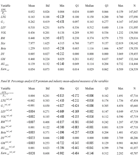
Panel A of Table 1 presents the descriptive statistics for the variable levels of the sample.
The mean and median of the proxy for analyst target E/P multiple, 𝐸𝐸𝐸𝐸𝐸𝐸1
𝐸𝐸�𝑖𝑖+1 , are 0.052 and 0.049,
respectively. Inverting the multiple, we find that half of the proxies for target P/E multiples are
equal to or above 20.41 and half are below. The mean and median of LTG are 0.163 and 0.150,
respectively. The mean and median of G2 are higher than those of LTG, at 0.262 and 0.163,
respectively. Panel B of Table 1 reports the descriptive statistics of the percentage E/P multiple
premium and the industry mean-adjusted growth, risk, and other variables.
Panel C of Table 1 shows the statistics for the measures of deviation for the variables in
panel A using their ten-year averages. The mean and median of �𝐸𝐸𝐸𝐸𝐸𝐸1 𝐸𝐸�𝑖𝑖+1�
𝐷𝐷𝑝𝑝𝐷𝐷_𝐻𝐻𝑖𝑖𝐻𝐻𝐻𝐻𝐷𝐷𝐻𝐻
are 0.012 and
0.010, respectively. The mean and median of LTGDev_HisAvg (–0.017 and –0.016) and those of
G2Dev_HisAvg(–0.049 and –0.025) are negative. This suggests that analyst expectations about the
22
brevity, we omit discussion of the other variables in the table.
Panel A of Table 2 presents the correlations between the industry mean-adjusted measures
and firms’ E/P multiple premiums relative to comparable firms �𝐸𝐸𝐸𝐸𝐸𝐸1 𝐸𝐸�𝑖𝑖+1�
𝑝𝑝𝑝𝑝𝑝𝑝𝑝𝑝𝑖𝑖𝑝𝑝𝑝𝑝
. As predicted, the
correlations between the E/P multiple premiums and the two growth premium measures and the
industry mean-adjusted gross margin ratio and the actual five-year sales growth rate are all
negative. The E/P multiple premiums are positively correlated with the industry-mean adjusted
financial leverage and book-to-market. The correlations between the E/P multiple premiums and
other measures of excess riskiness are not consistent with our predictions. Panel B of Table 2
presents the correlations between the measures that reflect deviations of variables from their
historical means. The correlations between �𝐸𝐸𝐸𝐸𝐸𝐸1 𝐸𝐸�𝑖𝑖+1�
𝐷𝐷𝑝𝑝𝐷𝐷_𝐻𝐻𝑖𝑖𝐻𝐻𝐻𝐻𝐷𝐷𝐻𝐻
and LTGDev_HisAvg and G2Dev_HisAvg are
negative, consistent with our prediction.
6. Empirical results
6.1 Results of tests of Hypotheses 1 and 1a
We estimate Equation (4) for both the pooled sample and the GICS sector subsamples to
analyse Hypotheses 1 and 1a. The Durbin-Watson statistics of the regressions we perform are
small, around 1.96. Following Petersen (2009), we address the dependence in the residuals by
clustering standard errors on firm and year dimensions. The results of the regression analyses for
the pooled sample are reported in panel A of Table 3.15 Models 1-3 in the panel analyses the
effects of the two growth premium measures on target P/E multiples with the risk and dividend
23
yield explanatory variables added in Model 4. Models 5 and 6 are designed to analyse the effect
of the three past performance measures.
In model 1, the coefficient of LTGind_adj(–0.255, t = –37.69) is statistically significant and
negative, and this result persists in models 3, 4, 5, and 6. In model 2, the coefficient of G2ind_adj
(–0.162, t = –56.88) is negative and statistically significant, and the result holds in models 3, 4,
5, and 6. In model 3, the coefficients of the two measures of growth premium remain negative
and significant.
GD suggest that market participants and analysts place excessive emphasis on firms’
near-term performance. The magnitude of the explanatory power of G2ind_adj (22%) in model 2
suggests that analysts do, in fact, place significant weight on the near term in their valuations.16
In model 4, the coefficient of LEVind_adj (0.188, t = 23.29) has the predicted sign and is
statistically significant, suggesting that, within the analyst’s industry coverage universe, firms
with higher financial risk receive higher E/P multiples. The coefficient of BMind_adj (0.141, t =
24.31) also has the predicted positive sign. The coefficient of Sizeind_adj (0.045, t = 2.27) has the
wrong sign and is also statistically significant at the 5 per cent level. This result suggests that, for
our sample period, analysts assigned lower E/P multiples to smaller firms within the analysts’
industry coverage universe. The result suggests that Lui et al.’s (2007) finding that risk
assessments of Salomon Smith Barney factor in size as a risk factor does not apply to our
sample. The coefficient of VOLind_adj (–0.038, t = –2.97) has the wrong sign and is statistically
16 It is important to note that this study does not attempt to compare the effects of G
2 and LTG on analyst target
P/E multiples. One needs to be cautious about making such a comparison for two reasons. First, there is not sufficient theoretical support for the argument that analysts place more weight on G2 than LTG. Existing evidence
(e.g., Bradshaw, 2004) suggests that long-term growth forecasts play an important role in analysts’ stock
24
significant. Additional analysis, however, reveals that this result is driven by observations in
years 2011 and 2013 during which the U.S. stock markets were exceptionally bullish. When
observations from years 2011 and 2013 are excluded, the (untabulated) coefficient of VOLind_adj
is not statistically significant, which may be attributable to the fact that the level of stock price
volatility is more informative than the industry mean-adjusted measure of the variable. For
example, Morgan Stanley analyst reports identify stocks that are expected to have more than a
25% chance of a price change (up or down) of more than 25% in a month as volatile stocks.
Betaind_adj (–0.001, t = –0.21) is not associated with the E/P multiple premiums in Model 4.
This result provides additional evidence that market beta appears not to be treated as a risk
measure in analysts’ analysis (e.g., Barker 1999a, Peasnell et al. 2016). Finally, the coefficient of
DYind_adj (0.015, t = 6.07) has the predicted positive sign and is statistically significant,
suggesting that firms expected to have a higher dividend yield receive higher E/P multiples than
comparable firms. In short, the results reported in model 4 provide strong support for Hypothesis
1.
Models 5 and 6 report the results of the regression analyses of the relationships between the
E/P multiple premiums/discounts assigned by analysts and firms’ relative measures of past
profitability, growth, and stability. In model 5, the coefficients of GMind_adj(–0.073, t = –8.16)
and AGsalesind_adj (–0.019, t = –7.29) both have the predicted negative signs, indicating that, other
things equal, firms with strong past profitability and growth tend to trade at higher earnings
multiples. The coefficient of Earnvolind_adj(–0.002, t = –0.55) has the wrong sign but is not
statistically significant. In model 6, the coefficients of GMind_adj and AGsalesind_adj have the
predicted negative sign but are not statistically significant. The coefficient of Earnvolind_adj(0.011,
25
that analysts assign higher E/P multiples to firms with higher past earnings volatility. In short,
the results reported in models 5 and 6 provide some support for Hypothesis 1a. Overall, the two
measures of future earnings growth have a substantial effect on analysts’ choices of target E/P
multiples while past profitability and past growth measures have a rather limited effect.
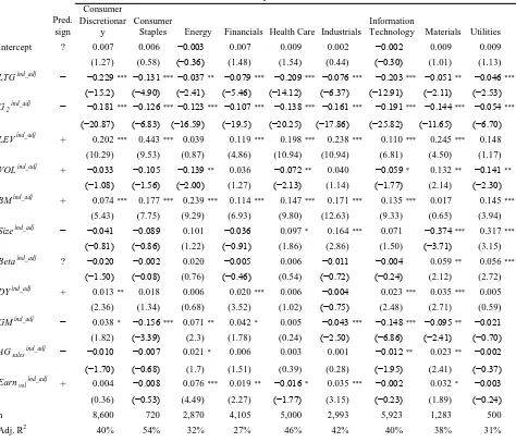
We also estimate Equation (4) for subsamples of the GICS sectors17 and the results are
reported in panel B of Table 3. Our finding that firms with more promising growth prospects
relative to comparable firms receive lower E/P multiples generally holds across all sectors.
�𝐸𝐸𝐸𝐸𝐸𝐸1
𝐸𝐸�𝑖𝑖+1�
𝑝𝑝𝑝𝑝𝑝𝑝𝑝𝑝𝑖𝑖𝑝𝑝𝑝𝑝
is negatively associated with G2ind_adj for all sectors reported in the panel. The
coefficient of LTGind_adj has the predicted negative sign and is statistically significant at least at
the 5 per cent level for all sectors. LEVind_adj has the predicted sign and is statistically significant
for seven out of the nine sectors. This suggests that analysts following most of the economic
sectors appear to discount financial risk in selecting target P/E multiples. BMind_adj has the
predicted positive sign and is statistically significant in eight of the nine regression tests.
The effects of the remaining risk measures vary across industry sectors. Sizeind_adj has the
predicted sign and is statistically significant for the materials sector. Betaind_adj has a positive sign
and is statistically significant at least at the 5 per cent level in the regression tests of the materials
and utilities sectors. The coefficient of VOLind_adj has the opposite sign to our expectations and is
statistically significant for four sectors, likely due to the fact that the level of stock price
volatility is more informative. The coefficient of GMind_adjis negative and significant at least at
the 1 per cent level for consumer staples, industrials, information technology, and materials
26
sectors. Earnvolind_adj has the predicted positive sign and is statistically significant at least at the
10 per cent level in four of the regression tests.
The adjusted R2s of the regression tests for the consumer discretionary, consumer staples,
healthcare, industries, information technology, and materials sectors are relatively high, ranging
from 0.38 to 0.54. This evidence mirrors the findings that analysts tend to apply earnings
multiples to firms in the consumer goods (retail), service, and industrial sectors (Barker 1999b,
Demirakos et al. 2004).18
6.2 Results of tests of Hypothesis 2
We estimate Equation (5) to test Hypothesis 2. The Durbin-Watson statistics of the tests we
perform are small, around 1.98. We address the dependence in the residuals by clustering
standard errors on firm and year dimensions. The results are reported in Table 4.
In model 1, the coefficient of LTGDev-HisAvg (–0.041, t = –11.64) is negative and statistically
significant. This result suggests that firms with more promising growth prospects in the next
three to five years relative to their long-runaverages receive lower E/P multiples from analysts
relative to the average forward E/P multiples at which they traded in the past. LTGDev-HisAvg
explains 2 per cent of the variation in the E/P multiple premiums assigned by analysts in model
1. The relatively low explanatory power of LTG may be attributable to the fact that analysts’
LTG forecasts are somewhat sticky.
In model 2, the coefficient of G2Dev-HisAvg (–0.031, t = –21.67) is also negative and statistically
27
significant. This suggests that firms that were expected to have higher near-term growth rates
than their long-run averages received lower E/P multiples from analysts relative to the average
historical forward E/P multiples at which they traded. G2Dev-HisAvg explains 11 per cent of the
variation in E/P multiple premiums assigned by analysts in model 2. In model 3, both growth
premium measures have the predicted negative sign.
In model 4, LEVDev-HisAvg (0.010, t = 3.09) is positively associated with the E/P multiple
premiums assigned by analysts. This suggests that analysts issue discounted valuation multiples
to firms with increased financial risk relative to their historical averages. The coefficient of
VOLDev-HisAvg (0.016, t = 11.84) has the predicted positive sign and is statistically significant. This
suggests that firms with higher levels of stock price volatility than their historical averages
received E/P multiples that were higher than the average historical forward E/P multiples at
which they traded. This result holds in model 6.
In model 4, the coefficient of BMDev-HisAvg (0.010, t = 4.37) has the predicted positive sign and
is statistically significant at the 1 per cent level. BetaDev_HisAvg is negatively associated with E/P
multiple premium. SizeDev_HisAvg has the wrong sign in all models. This suggests that, for our
sample period, increases in the firm’s market value appear to adversely affect analysts’ choices
of earnings multiples. However, it is possible that SizeDev_HisAvg simply captures fluctuations in
stock price over time rather than changes in riskiness or captures a number of firm-specific
factors, some of which could pull in the opposite direction. DYDev_HisAvg has the wrong sign and is
statistically significant at the 5 per cent level in model 4.
In model 5, the coefficients of GMDev_HisAvg (0.398, t = 6.48) and AGsalesDev-HisAvg (0.043, t =
10.84) are positive and statistically significant. This result suggests that firms with above
28
E/P multiples. One possible explanation for this result is that the analysts expect the high past
profitability and growth to decline over the longer run as profitability reverts to the mean, and
they assigned higher E/P multiples accordingly. EarnvolDev-HisAvg (–0.003, t = –0.24) has the
wrong sign but is not statistically significant in model 5.
In model 6, the results of the explanatory variables remain the same qualitatively. To
summarize, the results in Table 4 support Hypothesis 2 and suggest that analysts use historical
multiples of target firms to determine whether the P/E multiples they select for the firms are
outside historical norms, and whether the multiple premiums/discounts they assign are justified
by the firms’ fundamentals relative to historical averages.
7. Additional analysis
Analysts often reference the P/E multiples of broad market indexes such as the S&P 500 Index in
their research reports. We perform a preliminary analysis to provide some evidence on the
possible linkages between the benchmark market index P/E multiple and analysts’ choices of
target P/E multiples.
The S&P 500 forward P/E multiple reflects the market’s determination of how many times
expected earnings the 500 large U.S firms constituting the index should collectively trade. It can
serve as an additional benchmark in analysts’ valuation analysis in several ways. First, the
analyst may refer to the index’s P/E multiple and determine that a firm with fundamentals
stronger than the average performance of the S&P 500 firms should trade at a premium to the
P/E multiple for the S&P 500 Index, and vice versa. Second, the P/E multiples for the S&P 500
Index reflect the market’s expectations about the growth prospects of the U.S. economy and
29
prices, etc. (e.g., Reilly et al. 1983, White 2000). The macroeconomic data embedded in the
forward P/E multiples for the S&P 500 Index are logically valuable inputs into analysts’
projections of financial results, given that firms’ future fundamental performance (e.g., sales,
costs and earnings) are dependent on the growth prospects of the economy (e.g., the expected
GDP growth) and macroeconomic conditions (Lundholm and Sloan 2013).We expect analysts to
revise their expectations about firms’ growth and risk fundamentals, and hence their target P/E
multiples, subsequent to shifts in the levels of the S&P 500 P/E multiple driven by
macroeconomic developments. In addition, Campbell and Shiller (1988) show that the historical
average earnings of the S&P 500 Index help predict the present value of the future dividends of
the index. They find that as indicators of fundamental value relative to price, the E/P ratios of the
index predict one- to ten-years future returns. Thus, a low S&P 500 P/E ratio, and subsequent
increases in the ratio, may be interpreted by analysts as an indicator that the stock market is
currently undervalued and is in the process of adjusting to its fundamental value, and vice versa.
This may prompt analysts to adjust the valuation multiples for target firms accordingly.
For the above reasons, we conjecture that analysts revise their target E/P multiples in the
same direction as changes in the forward E/P multiple of the S&P 500 Index. We estimate the
following equation to test our prediction.
(6)
where the dependent variable represents the change in firm i’s target E/P multiple, which is the
difference between firm i’s target E/P multiple assigned by the analyst at time t and the previous
target E/P multiple assigned by the analyst. ΔSP500EPt represents the change in the forward E/P
multiple for the S&P 500 Index (SP500EP) in the date t calendar month. We predict that the
coefficient on ΔSP500EPt will be positive, reflecting analysts’ reactions to changes in the market
it it t
it t
it
Variables Control
EP SP P
EPS
ε β
α + ∆ + +
= ∆
+
500 )
ˆ
( 1
30
index P/E multiple. Our empirical model includes changes in the levels of the explanatory
variables from Equation (4) as control variables. Specifically, we include changes in the two
growth forecasts (ΔLTGit, ΔG2,it), changes in financial leverage, stock price volatility,
book-to-market, size, and market beta (ΔLEVit,ΔVOLit,ΔBMit, ΔLogMVit,and ΔBetait), and changes in the
dividend yield (ΔDYit) and the past performance measures (ΔGMit, ΔAGsales,it, ΔEarnvol,it).
We obtain information about the S&P 500 Index constituencies from COMPUSTAT. We
then collect three data items for each constituent firm from I/B/E/S: monthly consensus EPS1
forecast (EPS1i), the number of shares (Qi), and closing price (Pi) on the announcement day of
each month (the third Thursday). We calculate the E/P multiple (value-weighted) for the S&P
500 Index each month using the following formula:
𝐸𝐸𝑃𝑃500𝐸𝐸𝑃𝑃 =∑ 𝐸𝐸𝐸𝐸𝐸𝐸𝑖𝑖 1𝑖𝑖×𝑄𝑄𝑖𝑖
∑ 𝐸𝐸𝑖𝑖 𝑖𝑖×𝑄𝑄𝑖𝑖 (7)
Table 5 reports the results of our regression tests. We address the potential dependence in
residuals by clustering standard errors on firm and month dimensions. In model 1, the coefficient
of ΔSP500EP (0.423, t = 12.07) is positive and statistically significant. This suggests that
changes in the S&P 500 Index E/P multiples are associated with changes in analyst target E/P
multiples in the same direction. This single factor explains 5% of the variation in the changes of
analyst target E/P multiples. In model 2, the coefficients of ΔLTG (–0.023, t = –17.37) and ΔG2
(–0.024, t = –90.27) are negative and statistically significant. The coefficient of ΔSP500EP
remains positive and statistically significant in the presence of ΔG2 and ΔLTG.
In model 3, the result of ΔSP500EP remains unchanged qualitatively after the inclusion of
additional risk and past performance control variables. The results of the control variables are
largely consistent with those reported in Tables 3 and 4. In particular, increases in financial
31
revisions of analyst target E/P multiples. The change in market beta is positively associated with
the change in analyst target E/P multiples. However, the economic effect of the variable is quite
small.
8. Sensitivity tests
We performed several tests to assess the sensitivity of our results. First, we used the medians of
the forward E/P multiples and other measures as benchmarks to construct industry
median-adjusted measures. We then estimate Equation (4) using these variables and the results
(untabulated) are consistent with those reported in Table 3. We estimate Equation (4) using
industry mean-adjusted measures calculated based on the first and secondlevels of the GICS
industry classifications. Our results remained qualitatively unchanged. We also estimated
Equation (5) using the dependent and explanatory variables computed using five years of
historical data instead of ten years. The results again remained qualitatively unchanged but
slightly weaker.
Second, since our regression tests use individual analysts’ forecasts, there remains the
possibility that firms with high analyst following and analysts covering a large number of firms
may have disproportionate influence in our regression tests. Based on analyst following, for each
of the two samples used for estimating Equation (4) and Equation (5), we partition the sample
into two subsamples, one containing firms with the highest quartile of analyst following and the
other containing the remaining firms. We perform separate regression tests for the two
subsamples and the untabulated results reveal that the main inferences from our tabulated
findings also hold for both subsamples. We next partition each of our samples into two
32
analysts with the highest quartile of firm coverage and the other contains observations issued by
the remaining analysts. We conduct regressions for the subsamples and find that the untabulated
results reveal that the main inferences from our tabulated findings also hold for both subsamples.
We also partitioned samples using the medians of analyst following and analyst coverage and
find consistent results. To summarize, we find no evidence to indicate that the results of our
study are driven by firms with high analyst following or by analysts who cover a particularly
large number of firms.
Finally, we estimated Equation (4) and Equation (5) for a subsample that consists of firms in
consumer discretionary, consumer staples, and industrials sectors. Previous studies find that
analysts use the P/E multiple valuation method to value firms in those sectors. Thus, the
measurement errors in the proxies for analyst target E/P multiples, 𝐸𝐸𝐸𝐸𝐸𝐸1
𝐸𝐸�𝑖𝑖+1 , should be minimal for
this subsample, since dividing the EPS1 by target price forecast should provide an accurate
estimate of the E/P multiple applied by the analyst. The results (untabulated) based on the
subsample are consistent with those reported in panel A of Table 3 and Table 4. This suggests
that the potential impact of measurement errors in 𝐸𝐸𝐸𝐸𝐸𝐸1
𝐸𝐸�𝑖𝑖+1 on our findings appears to be limited.
9. Summary and conclusions
Prior literature has shown that analysts frequently use earnings-based multiples to value firms.
The present study uses a rigorous empirical approach based on valuation theory and evidence in
broker reports to examine closely the target P/E multiples that analysts apply in equity valuations
in order to derive a roadmap of how the multiples are actually arrived at. Our results indicate
that, contrary to assumptions of textbook authors and many researchers, analysts employ at least