Normal inverse Gaussian approximation for arrival time difference in flow induced molecular communications

warwick.ac.uk/lib-publications

Manuscript version: Author’s Accepted Manuscript

The version presented in WRAP is the author’s accepted manuscript and may differ from the

published version or Version of Record.

Persistent WRAP URL:

http://wrap.warwick.ac.uk/111713

How to cite:

Please refer to published version for the most recent bibliographic citation information.

If a published version is known of, the repository item page linked to above, will contain

details on accessing it.

Copyright and reuse:

The Warwick Research Archive Portal (WRAP) makes this work by researchers of the

University of Warwick available open access under the following conditions.

Copyright © and all moral rights to the version of the paper presented here belong to the

individual author(s) and/or other copyright owners. To the extent reasonable and

practicable the material made available in WRAP has been checked for eligibility before

being made available.

Copies of full items can be used for personal research or study, educational, or not-for-profit

purposes without prior permission or charge. Provided that the authors, title and full

bibliographic details are credited, a hyperlink and/or URL is given for the original metadata

page and the content is not changed in any way.

Publisher’s statement:

Please refer to the repository item page, publisher’s statement section, for further

information.

Normal Inverse Gaussian Approximation

for Molecular Communications

Werner Haselmayr

∗

,

Member, IEEE,

Dmitry Efrosin,

Member, IEEE,

Weisi Guo,

Member, IEEE

Abstract—The inverse Gaussian (IG) distribution is a well-established distribution for the first hitting time in flow-induced diffusion molecular communications. However, the distribution of the difference between two independent IG-distributed random variables has not been derived yet, although it is very important for the analysis of many molecular communication systems. For example, for deriving crossover probabilities or characterizing the noise in time between release modulation. In this letter, we propose an approximation by a normal inverse Gaussian (NIG) distribution and derive an asymptotic tail approximation. Nu-merical evaluations showed that the NIG approximation matches very well with the solution obtained through numerical integra-tion, in particular for the tails. Moreover, the asymptotic tail approximation converges very quickly to the actual probability and outperforms state-of-the-art tail approximations.

Index Terms—Molecular communications, flow-induced diffusion channel, normal inverse Gaussian distribution, inverse Gaussian distribution,

I. INTRODUCTION

M

communication broadly defines information transmis-sion using chemical signals [1]. It is a promising candidate for communications at nano-scale due to its ultra-high efficiency [2] and bio-compatibility. The main envisioned applications are in the area of nano-medicine [3] (e.g., targeted drug delivery). Currently, molecular communication research can be split into three areas: 1) Living system modelling

aims at gaining more insights into molecular communication processes occurring in biological live system using tech-niques originating from communications engineering (e.g., quantifying information in protein structures [4]) 2) Living systems interface aims to control the behavior of biological systems (e.g., connecting synthetic biology to electronics using redox modality [5]) 3) Artificial molecular communication

focuses on the design, fabrication and testing of human-made molecular communication systems (e.g., artificial chemical communication between gated nanoparticles [6]).

In molecular communications the information can be en-coded using molecule’s concentration [7], number [8], release time [9], type [10] or a combination of the aforementioned methods. The information molecules can be transported from the transmitter to the receiver through pure diffusion, diffu-sion with flow, active transport (e.g., molecular motors [11]) and bacteria [12]. Most molecular communication research

Manuscript received month day, 2018; revised month day, 2018; ac-cepted month day, 2018. ∗Corresponding author. W. Haselmayr and D. Efrosinin are with the Johannes Kepler University Linz, Austria (email: [email protected]; [email protected]). W. Guo is with the School of Engineering, University of Warwick, United Kingdom (email: [email protected]).

is devoted to diffusion-based molecular communication. In this case the receiver can be classified as either passive or active [13]. Typically a passive receiver only observes the molecules in the environment, but does not react with the information molecules. In contrast, for active receiver a chemical reaction between receiver and molecules takes place and the molecules is recognized by the receiver due to the reaction. The first hitting time in pure diffusion and flow-induced diffusion channels with an active (absorbing) re-ceiver [14] can be modelled by a Lévy [15] and inverse Gaus-sian (IG) [9] distribution, respectively. The difference between two independent Lévy-distributed random variables follows a stable distribution [15]. This distribution is very important in order to characterize crossover probabilities [8], [16], [17] and noise in time between release modulation [15] for pure diffusion channels. However, to the best of our knowledge the distribution of the difference between two IG-distributed random variables has not been derived yet. So far, only an asymptotic tail approximation was proposed in [16].

In this letter, we present an approximation of the distribution of the difference between two IG-distributed random variables by a normal inverse Gaussian (NIG) distribution. Through mo-ment matching we derive closed-form expressions for the four parameters of the NIG distribution. Moreover, we derive an asymptotic tail approximation. Numerical evaluations showed that the NIG approximation matches very well with the results obtained through numerical integration, in particular for the tails. The tail approximation converges much faster than the state-of-the-art approximation proposed in [16].

II. INVERSEGAUSSIANDISTRIBUTION

In this section, we briefly discuss the main properties of the inverse Gaussian (IG) distribution1. The probability density function (PDF) of an IG-distributed random variableX is given by [18]

fX(x)= a

√ 2π

exp(ab)x−3/2exp −1 2

a2x−1+b2x !

, x>0,

(1)

with the parameters a > 0 and b > 0. We indicate an IG-distributed random variable with the parameters (a,b) by

X ∼IG(a,b). The cumulative distribution function (CDF) can be expressed as

FX(x)=φ

(bx)1/2−ax−1/2+exp (2ab)

+φ

−(bx)1/2−ax−1/2, x>0, (2)

with the CDF of the standard normal distribution φ(x)=1/√2π_−∞x exp(−t2/2)dt. Moreover, the tail probability is given by ¯FX(x) = 1 −FX(x). The moment-generating function of X can be expressed as

MX(t)=exp

ab−apb2_{−2t. (3)}

It is important to note that the IG distribution is only closed under convolution, i.e. the linear combination of IG-distributed random variables is also IG-IG-distributed, if certain conditions are fulfilled [18]. Suppose V = PN

i=1ciXi, with Xi =IG(ai,bi), ci > 0 and all Xi are independent. The

random variable V is only IG-distributed, iff bi/

√

ci =c for

alli. Then the moment-generating function ofV is given by

MV(t)= N Y

i=1

MXi(cit)

= N Y

i=1 exp

ai

bi−

q b2

i −2cit

=exp* ,

N X

i=1

ai√ci

c− pc2_−2t+

-. (4)

Thus,V ∼IGPN i=1ai

√

ci,c

. The constancy of bi/

√

ci is a

necessary condition for V to be IG-distributed.

III. NORMALEINVERSEGAUSSIANAPPROXIMATION

Let’s consider a random variable Z = X1 − X2, with

X1∼IG(a1,b1) and X2 ∼ IG(a2,b2). Assuming X1 and X2 are independent the PDF of Z can be expressed as

fZ(z)=

fX1∗f − X2

(z)=

∞

−∞

fX1(u)fX2(u−z)du, (5)

with f_X−

2 = fX2(−x). The moment-generating function ofZ is

given by

MZ(t)=MX1(t)MX2(−t)

=exp

a1b1+a2b2−

a1

q

b2₁−2t+a2

q

b2₂+2t .

(6)

Since b1 , b2 the random variable Z is not IG-distributed (cf. Sec. II). Although the moment-generating function of Z can easily be derived, the PDF of Z is difficult to analyze. Moreover, to the best of our knowledge, neither a closed-form expression nor an approximation has been derived so far. In the following we propose the normal inverse Gaussian (NIG) distribution as an appropriate approximation for Z, since the NIG distribution is a flexible system of dis-tributions, including heavy-tailed and skewness distributions. The NIG approximation was introduced in [19] and it was shown through numerical results that NIG approximation has a smaller approximation error compared to Gram-Charlier expansion [20] and Edgeworth expansion [21].

The PDF of a NIG-distributed random variableY is defined by [19]

fY(y)=αδ

π exp δ

q

α2₋β2₋β_(y−µ₎

!

×

K1

αp

δ2_+(y−µ)2

p_δ2

+(y−µ)2 , (7) with the parameters α > 0, δ > 0, µ ∈ _R and 0 ≤ |β| < α and K1(·) denotes the modified Bessel function of the third kind with index 1. The parameters α, β, µ and δ determine the tail heaviness, asymmetry, location and scaling of the distribution. The Gaussian distribution arises as a special case of the NIG distribution by settingα→ ∞,β=0 andδ=σ2α, where σ2 denotes the variance of the Gaussian distribution. The relation between meanM, variance V, skewnessS and excess kurtosis K ofY is given by [19]

α=3ρ1/2(ρ−1)−1V−1/2|S |−1

β=3(ρ−1)−1V−1/2S−1

µ=M −3ρ−1V1/2S−1

δ=3ρ−1(ρ−1)1/2V−1/2|S |−1,

(8)

where ρ=3K S−2_−4>1.

We approximate the unknown distribution of Z by matching the mean, variance, skewness and excess kurtosis of Z with the NIG distribution, which is known as moment matching method [22]. The moments are then used to derive the pa-rameters α, β, µandδ according to (8). The mean, variance, skewness and excess kurtosis of Z can be expressed in terms cumulants

ˆ

M =κ₁, Vˆ =κ₂,

ˆ

S= κ3

κ3/2

2

, _Kˆ ₌ κ4

κ2

2

. (9)

where κn, n = 1. . . ,4, denotes the nth cumulant of Z.

The cumulants can be derived using the moment-generating function of Z defined in (6)

κn =

∂n

∂tnlnMZ(t)

t=0

. (10)

In the following we present the analytical expressions for the parametersα, β,µandδfor two important cases in molecular communications.

A. Case 1: a1=a2=a and b1=b2 =b

In this case the moment-generating function of Z can be written as

MZ(t)=MX1(t)MX2(−t)

=exp

ab+ab−

apb2_−2t+_ap_b2+_2t . ₍₁₁₎

The moments are obtained by applying (10) and (9)

ˆ

M=0, Vˆ =2a

b3, ˆ

S=0, Kˆ = 15

2ab.

The parameters of the corresponding NIG distribution can be derived using the relation in (8) and can be expressed as

α= √b2

5, β=0,

µ=0, δ= √2

5

a b.

(13)

The resulting NIG distribution is symmetric, since β=0.

B. Case 2: b1/a1=b2/a2=c

In this case the moment-generating function of Z can be written as

MZ(t)=MX1(t)MX2(−t)

=exp

a2₁+a₂2c−

a1

q a2

1c2−2t+a2

q a2

2c2+2t . (14)

Similar to case 1, the moments can be calculated using (10) and (9)

ˆ

M=0, Vˆ = a

−2

1 +a

−2 1

c3 ,

ˆ

S= 3

a−₁2+a−₁2 q

ca−₁2+a−₁23

, Kˆ =15

a₁−6+a−₁6

ca₁−2+a−₁22

. (15)

The parameters of the corresponding NIG distribution can be expressed as

α=

a₁2−a2₂2 q

a4₁+3a₁2a2₂+a₂4 a2₁−a₂2−2|τ|

5a2 1a22

q a−2

1 +a

−2 2

c−3

,

β=

−a2₁+a₂2c2

5 ,

µ= a

4 1−a

4 2

a₁4+3a₁2a2₂+a₂4c

,

δ=

√ 5a2₁a2₂

q a−2

1 +a

−2 2

c−3_|τ_|

q

a2₁a₂2a₁2−a2₂−2(a4₁+3a2₁a₂2+a4₂) ,

(16)

with

τ=

a−2

1 +a

−2 2

3/2 √ c

a−₁4−a−₂4 .

The NIG distribution is asymmetric, since β,0.

IV. TAILAPPROXIMATION

The tail probability of the random variable Z, defined in (5), is given by

¯

FZ(z)=Pr(Z >z)= ∞

z

fZ(t)dt

= ∞ z ∞ −∞

fX1(u)fX2(u−t)dudt

= ∞ z ∞ −∞

fX1(v+t)fX2(v)dvdt

= ∞

−∞ fX2(v)

∞

z

fX1(v+t)dtdv

= ∞

−∞

fX2(v) ¯FX1(v+z)dv. (17)

The asymptotic tail behavior can be derived as follows

lim

z→∞

¯

FZ(z)

¯

FX1(z) = lim

z→∞ ∞

−∞

fX2(v) ¯FX1(z+v)

¯

FX1(z)

dv = ∞ −∞ lim z→∞ ¯

FX1(z+v)

¯

FX1(z)

fX2(v)dv

= ∞

−∞

exp−b2₁/2v fX2(v)dv, (18)

where we used limz→∞FX¯ 1(z+v)/FX¯ 1(z)=exp(−b

2 1/2v) for allvreal [23]. Thus, the asymptotic tail behavior ofZ is given by

lim

z→∞

¯

FZ(z)=F¯X1(z) ∞

−∞

exp−b2₁/2v fX2(v)dv

=_F¯_X

1(z)MX2(−b

2

1/2), (19)

whereMX1(x) denotes the moment-generating function of the

inverse Gaussian distribution defined in (3).

V. APPLICATIONS INMOLECULARCOMMUNICATIONS

For molecular communications in flow-induced diffusion channels, the random time between the release of molecules until the first arrival at an absorbing receiver [14] can be modelled as IG-distributed random variable – so-called first hitting time. In the following, we discuss two applications showing the importance of knowing the distribution of the difference between two independent IG-distributed random variables.

A. Timing Channels

TABLE I

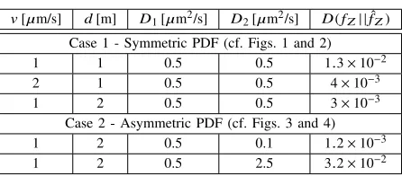
KL DIVERGENCE PERFORMANCE OF THENIGAPPROXIMATION v[µm/s] d[m] D1[µm2/s] D2[µm2/s] D(fZ| |fˆZ)

Case 1 - Symmetric PDF (cf. Figs. 1 and 2) 1 1 0.5 0.5 1.3×10−2 2 1 0.5 0.5 4×10−3

1 2 0.5 0.5 3×10−3

Case 2 - Asymmetric PDF (cf. Figs. 3 and 4) 1 2 0.5 0.1 1.2×10−3 1 2 0.5 2.5 3.2×10−2 at time S is given byY = S+X, where X denotes the first hitting time and follows an IG distribution. If the information is encoded inZs =S2−S1, where S1andS2denote the release time of the individual molecules, the channel model is given by [15]

Y2−Y1 =S2−S1+X2−X1

Zy=Zs+Zx, (20)

with the noise term Zx = X2 −X1 and X1 and X2 are IG-distributed random variables. In order to analyze such timing channels the distribution of Zx is of interest. Since the exact

distribution of Zxis hard to determine, it can be approximated

by a NIG distribution (Sec. III).

B. Crossover Probability

Let’s assume that two molecules of different type, representing bit 0 and bit 1, are released a time intervalT apart. The first hitting time of the first and second transmitted molecules is given by X1 and X2, respectively, and follow an IG distri-bution. The probability for the released molecules to arrive out-of-order can be expressed as

Pr(X1−X2>T)=Pr(Zx >T), (21)

which is referred to as crossover probability. In order to evaluate the crossover probability in (21) the distribution ofZx

is of interest. Since the exact distribution of Zx is hard to

determine, a possible solution is to approximate Zx by a

NIG distribution (cf. Sec. III). It is important to note that the crossover probability in (21) is frequently used for the theoretical analysis of molecular molecular communication systems. For example, based on the crossover probability an approximated error performance for different channel coding techniques was presented in [16] and the channel capacity for binary molecule shift keying was derived in [17].

VI. NUMERICALEVALUATION

For the numerical evaluation we consider molecular communi-cations in a semi-infinite one-dimensional (1D) fluidic environ-ment (e.g., blood vessel) between a receiver and a transmitter that are placed at a distanced. Moreover, we assume a positive flow with velocity v from transmitter to receiver. For such a flow-induced diffusion channels the first hitting time of a released molecule at an absorbing receiver [14] follows an IG distribution.

-10 -5 0 5 10

z 0

0.1 0.2 0.3 0.4 0.5

fZ

(z)

[image:5.612.62.285.79.177.2]

v=1µm/s, d=1m v=2µm/s, d=1m v=1µm/s, d=2m

Fig. 1. Probability density function ofZ=X1−X2for case 1 (cf. Sec. III-A).

The solid lines indicate the PDF obtained through numerical integration of (5) and the dashed lines correspond to the NIG approximation with the parameters in (13).

Figs. 1 – 4 show the PDF and the tail probability of the random variable Z = X1 −X2, where X1 and X2 are IG-distributed random variables with the parameters

a1=

d

√ 2D1

, a2 =

d

√ 2D2

,

b1= v √

2D1

, b2 =

v √

2D2

, (22)

where D1 and D2 denote the diffusion coefficients of the released molecules. In Figs. 1 – 4 the solid lines indicate the results obtained through numerically integration of (5) and the dashed lines correspond to the NIG approximation. Moreover, the dotted lines in Figs. 2 and 4 represent the asymptotic tail behavior. Moreover, we use the Kullback-Leibler (KL) divergence to evaluate the performance of the NIG approximation. The KL divergence between the actual distribution fZ(z), obtained through numerical integration

of (5), and the NIG approximation ˆfZ(z) can be calculated

by [24]

DfZ||fˆZ

= ∞

−∞

fZ(z)ln fZ(z)

ˆ

fZ(z)

dz. (23)

The KL divergence of different scenarios is summarized in Tab. I.

In Figs. 1 and 2 the PDF and tail probability for case 1 (cf. Sec. III-A) are shown. In this case

a1=a2=d/ √

2D1 and b1 = b2 = v/ √

2D1, with

1 3 5 7 9 z

0 0.1 0.2 0.3

Pr(Z > z)

v=1µm/s, d=1m v=2µm/s, d=1m v=1µm/s, d=2m

0 0.5 1

[image:6.612.65.287.52.217.2]

0 0.25 0.5

Fig. 2. Tail probability of Z = X1−X2 for case 1 (cf. Sec. III-A). The

solid lines indicate the tail obtained through numerical integration of (17), the dashed lines correspond to the tail probability of the NIG approximation with the parameters in (13) and the dotted lines represent the asymptotic tail behavior derived in (19).

-10 -5 0 5 10

z 0

0.1 0.2 0.3 0.4

fZ

(z)

[image:6.612.327.550.53.217.2]

D1=0.5µm2/s, D2=0.5µm2/s D1=0.5µm2/s, D2=0.1µm2/s D1=0.5µm2/s, D2=2.5µm2/s

Fig. 3. Probability density function ofZ=X1−X2for case 2 (cf. Sec. III-A).

The solid lines indicate the PDF obtained through numerical integration of (5) and the dashed lines correspond to the NIG approximation with the parameters in (16).

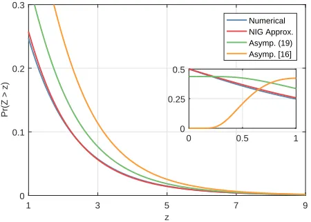
observe a positive skew (right tail is longer) if D2 becomes smaller compared to D1 and a negative skew (left tail is longer) if D2 becomes larger compared to D1. We observe a very good match between the numerical solution and the NIG approximation, in particular for the tails, and the asymptotic tail approximation quickly converges to the actual probability. In Fig. 5 we compare the asymptotic tail approximation in (19) with a recently proposed tail approximation given by [16]

¯

FZ(z)=4D1

v2 exp

* .

,

√

2−1dv 2D1

+ /

-fX1(x), (24)

where fX1(x) denotes the PDF of an IG distribution defined

in (1). We observe that asymptotic tail approximation in (19) converges much faster than the approximation in (24). More-over, the approximation in (24) is only valid if the PDF is symmetric, whereas the approximation in (19) can also be applied to asymmetric PDFs.

1 3 5 7 9

z 0

0.1 0.2 0.3

Pr(Z > z)

D1=0.5µm2/s, D2=0.5µm2/s D1=0.5µm2/s, D2=0.1µm2/s D1=0.5µm2/s, D2=2.5µm2/s

0 0.5 1

[image:6.612.326.551.279.440.2]

0 0.25 0.5

Fig. 4. Tail probability of Z = X1−X2 for case 2 (cf. Sec. III-B). The

solid lines indicate the tail obtained through numerical integration of (17), the dashed lines correspond to the tail probability of the NIG approximation with the parameters in (16) and the dotted lines represent the asymptotic tail behavior derived in (19).

1 3 5 7 9

z 0

0.1 0.2 0.3

Pr(Z > z)

Numerical NIG Approx. Asymp. (19) Asymp. [16]

0 0.5 1

0 0.25 0.5

Fig. 5. Tail probability comparison for case 1 (cf. Sec. III-A), with

v=1µm/s,d=2µm andD1=0.5×10−12µm2/s.

VII. CONCLUSIONS

In this letter, we have proposed an approximation for the distribution of the difference between two independent IG-distributed random variables. We derived the four parameters of the NIG distribution through the moment matching method. Moreover, we have presented an asymptotic tail tion. We have shown numerically that the NIG approxima-tion matches very well with the results obtained through numerically integration and the asymptotic tail approximation converges quickly to the actual probability. It is important to note that the proposed approximations are very important for the analysis of flow-induced diffusive molecular communi-cations. For example, for deriving crossover probabilities or characterizing the noise in time between release modulation.

REFERENCES

[1] N. Farsad, H. B. Yilmaz, A. Eckford, C. B. Chae, and W. Guo, “A comprehensive survey of recent advancements in molecular communi-cation,”IEEE Commun. Surveys Tuts., vol. 18, no. 3, pp. 1887–1919, thirdquarter 2016.

[image:6.612.62.290.286.444.2]

[3] L. Felicetti, M. Femminella, G. Reali, and P. Lió, “Applications of molecular communications to medicine: A survey,” Nano Commun. Netw., vol. 7, pp. 27 – 45, 2016.

[4] R. Huculeci, E. Cilia, A. Lyczek, L. Buts, K. Houben, M. A. Seeliger, and T. Lenaerts, “Dynamically coupled residues within the SH2 domain of FYN are key to unlocking its activity,”Structure, vol. 24, pp. 1947 – 1959, 2016.

[5] Y. Liu, J. Li, T. Tschirhart, J. L. Terrell, E. Kim, C.-Y. Tsao, D. L. Kelly, W. E. Bentley, and G. F. Payne, “Connecting biology to electronics: Molecular communication via redox modality,” Advanced Healthcare Materials, vol. 6, no. 24, pp. 1 700 789 – 1 700 807, 2017.

[6] A. Llopis-Lorente, P. Diez, A. Sanchez, M. D. Marcos, F. Sancenon, P. Martinez-Ruiz, R. Villalonga, and R. MartÃnez-Manez, “Interactive models of communication at the nanoscale using nanoparticles that talk to one another,”Nature Commun., pp. 1–7, 2017.

[7] M. S. Kuran, H. B. Yilmaz, T. Tugcu, and I. F. Akyildiz, “Interference effects on modulation techniques in diffusion based nanonetworks,”

Nano Communication Networks, vol. 3, no. 1, pp. 65 – 73, 2012. [8] Y. K. Lin, W. A. Lin, C. H. Lee, and P. C. Yeh, “Asynchronous

threshold-based detection for quantity-type-modulated molecular communication systems,”IEEE Trans. Mol., Biol. Multi-Scale Commun., vol. 1, no. 1, pp. 37–49, March 2015.

[9] K. V. Srinivas, A. W. Eckford, and R. S. Adve, “Molecular communica-tion in fluid media: The additive inverse Gaussian noise channel,”IEEE Trans. Inf. Theory, vol. 58, no. 7, pp. 4678–4692, July 2012. [10] N. R. Kim and C. B. Chae, “Novel modulation techniques using isomers

as messenger molecules for molecular communication via diffusion,” in

Proc. IEEE Int. Conf. on Commun., June 2012, pp. 6146 – 6150. [11] N. Farsad, A. W. Eckford, and S. Hiyama, “A mathematical channel

optimization formula for active transport molecular communication,” in

Proc. IEEE Int. Conf. on Commun., June 2012, pp. 6137 – 6141. [12] S. Qiu, W. Haselmayr, B. Li, C. Zhao, and W. Guo, “Bacterial relay for

energy-efficient molecular communications,”IEEE Trans. Nanobiosci., vol. 16, no. 7, pp. 555 – 562, Oct 2017.

[13] A. Noel, Y. Deng, D. Makrakis, and A. Hafid, “Active versus passive: Receiver model transforms for diffusive molecular communication,” in

Proc. IEEE Global Commun. Conf., Dec 2016, pp. 1 – 6.

[14] H. B. Yilmaz, A. C. Heren, T. Tugcu, and C. B. Chae, “Three-dimensional channel characteristics for molecular communications with an absorbing receiver,”IEEE Commun. Lett., vol. 18, no. 6, pp. 929–932, June 2014.

[15] N. Farsad, W. Guo, C. B. Chae, and A. Eckford, “Stable distributions as noise models for molecular communication,” inProc. IEEE Global Commun. Conf., Dec 2015, pp. 1–6.

[16] P. J. Shih, C. H. Lee, P. C. Yeh, and K. C. Chen, “Channel codes for reliability enhancement in molecular communication,”IEEE J. Sel. Areas Commun., vol. 31, no. 12, pp. 857–867, Dec 2013.

[17] Y.-P. Hsieh, Y.-C. Lee, P.-J. Shih, P.-C. Yeh, and K.-C. Chen, “On the asynchronous information embedding for event-driven systems in molecular communications,”Nano Comm. Netw., vol. 4, pp. 2–13, 2013. [18] R. S. Chhikara and J. L. Folks, The Inverse Gaussian Distribution: Theory, Methodology, and Applications. New York, NY, USA: Marcel Dekker, Inc., 1989.

[19] A. Eriksson, E. Ghysels, and F. Wang, “The normal inverse Gaussian distribution and the pricing of derivatives,” Journal of Derivatives, vol. 16, no. 3, pp. 23–37, 3 2009.

[20] C. V. L. Charlier, “Über die Darstellung willkürlicher Funktionen,”Ark. Mat. Astr. och Fysic 2, 1905.

[21] F. Y. Edgeworth, “On the representation of statistical frequency by a series,”Journal of the Royal Statistical Society, vol. 70, no. 1, pp. 102– 106, 1907.

[22] N. I. Akhiezer,The classical moment problem and some related ques-tions in analysis. London, UK: Oliver and Boyd, 1965.

[23] P. Embrechts, “A property of the generalized inverse Gaussian distribu-tion with some applicadistribu-tions,”Journal of Applied Probability, vol. 20, no. 3, pp. 537 – 544, 9 1983.